Measuring the quasar luminosity function below the detection threshold

Masters’ Thesis

Measuring the quasar luminosity function

below the detection threshold

Author:

Eliab Malefahlo

Supervisors: Prof Mario Santos Dr Jonathan Zwart Prof Matt Jarvis Prof Roy Maartens

A thesis submitted in fulfilment of the requirements for the degree of Msc Astronomy

in the

Astronomy group

Department of Physics and Astronomy

March 2016        

Declaration of Authorship

I, Eliab Malefahlo, declare that this thesis titled, ’Measuring the quasar luminosity function below the detection threshold’ and the work presented in it are my own. I confirm that:

This work was done wholly or mainly while in candidature for a research degree at this University. Where any part of this thesis has previously been submitted for a degree or any other qualification

at this University or any other institution, this has been clearly stated.

Where I have consulted the published work of others, this is always clearly attributed.

Where I have quoted from the work of others, the source is always given. With the exception of

such quotations, this thesis is entirely my own work.

I have acknowledged all main sources of help.

Where the thesis is based on work done by myself jointly with others, I have made clear exactly

what was done by others and what I have contributed myself.

Signed: Date: ii      

University of the Western Cape

Abstract

FACULTY NATURAL SCIENCE Department of Physics and Astronomy

Msc Astronomy

Measuring the quasar luminosity function below the detection threshold by Eliab Malefahlo

The radio emission of radio-quiet active galactic nuclei (AGN) is thought to be from star formation and AGN related emission. I investigate these sources using 1.4 GHz radio data from FIRST and three optical quasars samples from the SDSS: (i) a volume-limited sample in the redshift range 0.2< z <0.4 defined by Mi < −23 (ii) magnitude-limited sample in the redshift range 1.8 < z < 2.5 defined by

mr ≤ 18.5 and (iii) a uniform sample in the redshift range 0.2 < z < 3.5 (divided into 12 redshift

bins). I constructed radio source counts and radio luminosity functions (RLFs) using the optical quasars detected in FIRST, which are consistent with literature results obtained using SDSS and NVSS quasars. There are differences at the low fluxs end because of the different resolutions of FIRST and NVSS. I applied a median stack method to the 12 redshift bins of the uniform sample and found that the median flux decreases from 182 µJy in the lowest redshift bin to 39 µJy and the highest redshift bin. This is because the high redshift quasars although more luminous than their low redshift counterparts, they are much further away so they have lower fluxes. I probed the quasar radio source counts to lower levels using reconstructed source counts obtained by applying the Bayesian stack technique. The reconstructed radio source counts were then used to constructed the quasar RLF to lower levels, where I found: (i) for z < 1 the constructed quasar RLF has the same slope as the detected quasars, suggesting that like the detect quasars their radio emission is dominated by AGN related emission (ii) above z = 1 the constructed RLF steepens with redshift, which suggests the strong link between accretion rate and radio jet power is gradually breaking down towards faint optical luminosities at high redshift.

I would firstly like to thank my living God for the life and health He has and continues to bless me with, for granting me this opportunity, the power and strength to complete this work. Ke ya moleboga Modimo wa Sethepu, Mambo wamazimambo, Senatla sa dinatla Ntate Moemedi. I would like to thank my superiors; Mario, Jon (JZ), Matt and Roy for being there and always willing to help, going through the concepts step by step and letting me figure things on my own were needed. This work would not be possible without them. Thanks you JZ for all those hours of explaining the code and proofreading my work thanks chief. I would like to thank my parents for their love and continued support. Thanks Matt Prescott for all those LFs sessions. I would also like to thank my fellow students in the Astro group at UWC for their support, especially Rudi-Lee and my home boy Emanuel. Lastly, I would like to thank Neville for all the advice and motivation. I thank the National astrophysics and space science program (NASSP) and SKA Africa for financial assistance during my studies. The authors thankfully acknowledge the computer resources, technical expertise and assistance provided by CENTRA/IST. Computations were performed at the cluster “Baltasar-Sete-S´ois” and supported by the H2020 ERC Consolidator Grant ”Matter and strong field gravity: New frontiers in Einstein’s theory” grant agreement no. MaGRaTh-646597.

iv        

Contents

1.1.1 Evolution of the Universe . . . 2

1.1.2 Galaxy formation and evolution. . . 4

1.2 Galactic processes . . . 5

1.2.1 Star formation . . . 6

1.2.2 Active galactic nuclei . . . 6

1.2.3 Feedback . . . 8

1.2.4 Synchrotron radiation . . . 9

1.2.5 Far-Infrared Radio correlation. . . 9

1.3 Radio sources . . . 10

1.3.1 Radio-loud . . . 11

1.3.2 Radio-quiet . . . 11

1.4 Quasars . . . 11

1.5 Large radio surveys . . . 12

1.6 Outline . . . 13 2 Data 15 2.1 SDSS . . . 15 2.1.1 SDSS I . . . 15 2.1.2 SDSS II . . . 15 2.1.3 SDSS III . . . 17

2.1.4 Quasar target selection: SDSS I and II . . . 18

2.1.5 Quasar target selection: SDSS III. . . 19

2.1.6 Spectroscopy . . . 21 2.1.7 Quasar catalogue . . . 23 v      

2.2 Sample. . . 23

2.2.1 Sample 1: Volume-limited sample. . . 23

2.2.2 Sample 2: Magnitude-limited sample . . . 23

2.2.3 Sample 3: Uniform sample . . . 24

2.2.4 Completeness . . . 24

2.3 FIRST . . . 25

2.4 Matching SDSS with FIRST. . . 26

2.4.1 Catalogue sources . . . 26

2.4.2 FIRST cutouts . . . 27

2.5 Catalogue and extracted fluxes . . . 27

2.5.1 Snapshot bias . . . 28

2.5.2 Extraction position. . . 29

2.6 Sample area . . . 29

2.6.1 BOSS overlap . . . 29

2.6.2 Legacy overlap . . . 31

3 Above the detection threshold: Radio-loud quasars 32 3.1 Source counts . . . 32

3.1.1 Sample 1 . . . 35

3.1.2 Sample 2 . . . 36

3.2 Radio luminosity function . . . 36

4 Below the detection threshold: stacking and radio-quiet quasars 40 4.1 Stacking . . . 41

4.2 Sample 3: Uniform sample . . . 41

4.3 Simple averaging . . . 42

4.4 Bayesian framework . . . 43

4.4.1 Bayes’ theorem . . . 43

4.4.2 Nested sampling . . . 45

4.4.3 Models considered here . . . 45

4.4.4 Likelihood. . . 46

4.4.5 Priors . . . 47

4.4.6 Tests and simulations . . . 48

4.5 Results. . . 48

4.5.1 Posterior distributions . . . 51

4.5.2 Source counts . . . 51

4.5.3 Luminosity functions. . . 52

5 Conclusions and future work 61 5.1 Future work . . . 63 Bibliography 64        

Chapter 1

Introduction

In this thesis, I use a Bayesian stacking (Bayestack) technique to extend measurements of the quasar radio luminosity function (QRLF) and source counts of optically selected sources below the detection threshold of currently completed large-area radio surveys. I use the results to investigate the role of star formation and active galactic nuclear accretion (AGN) activity on the radio emission of quasars, in particular the radio-quiet quasars. First, I explore the importance of these two sources of emissions for galaxy formation and evolution.

1.1

Cosmological context

1.1.1 Evolution of the Universe

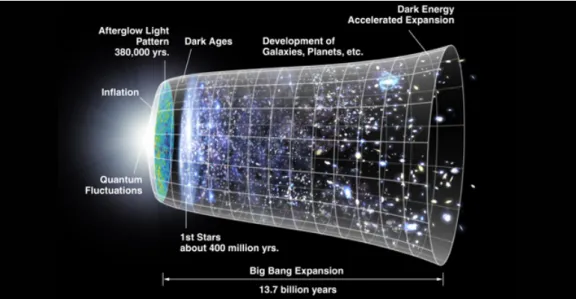
The Big Bang theory is the most accepted evolutionary model of the Universe (see Peebles and Ratra [2003] for an overview). The theory states that the Universe originated from a singularity with infinite temperature and density, expanding to what is observed today (assuming general relativity holds in the early Universe; Hawking and Ellis[1973]). The Universe expanded and cooled growing exponentially in size over a short time scale 10−33 to 10−32 (inflation; e.g. Guth and Jagannathan [1998]). After inflation, elementary particles were formed and as the Universe continued to expand and cool some particles combined to form nucleons. Around 380,000 years after the Big Bang, the Universe became cool enough for atoms to form, making the Universe transparent because the free electrons that were scattering photons were captured to form these atoms (recombination).

The Big Bang model is a solution to Einstein’s field equations by Alexander Friedman where he as-sumed an isotropic and homogeneous space on large scales. One of the strongest pieces of evidence supporting the model is the prediction of the Cosmic Microwave Background (CMB, Penzias and Wilson[1965]) radiation, the thermal afterglow of the Universe after recombination. The background

2      

Figure 1.1: An artist impression on the time scale of the evolution of the Universe according to the

Big Bang model. (NASA/WMAP science team).

radiation is an almost perfectly uniform blackbody with temperature fluctuations of the order 10−5 (Smoot et al. [1992]). Further evidence for the Big Bang includes; the expansion of the Universe (i.e. Hubble’s law; Hubble [1929]) and the abundance of elements observed today (Alpher et al. [1948]). Measurements of the fluctuations in the CMB together with galaxy distribution measured in galaxy surveys place tight constraints on the cosmological parameters and favours the so-called ΛCDM model. This is parameterized with four types of matter: dark matter, baryonic matter, hot dark matter (ra-diation) and dark energy, the latter component dominates the current energy budget of the Universe and is responsible for the accelerated expansion of the Universe. The latest results from Planck Col-laboration et al. [2015] give a Hubble constant, H0 = 67.8±0.9 km s−1Mpc−1 and a dark matter

density, Ωm = 0.308±0.012. The model, however, is not perfect and in solving some of its problems

other problems arise.

The problems with the ΛCDM model arises when there is discrepancy between its predictions and observations. This leads to the introduction of quantities such as dark matter and dark energy to account for this discrepancy. Dark matter is used to account for the missing mass needed to explain the kinetic motions observed (i) from rotation curves of stars orbiting galactic centres (Rubin et al. [1980]) and (ii) in galaxies rotating about the centre of mass of their clusters (Zwicky [1937]). Dark matter makes up ≈ 90% of matter and only interacts gravitationally, possibly weakly as well, with baryonic matter but does not absorb or emit electromagnetic radiation. Dark energy is the term given to the mysterious force pushing the expansion of the Universe in spite the gravitational force (Lemaˆıtre [1927],Hubble[1929]). It has recently been found that not only is the Universe expanding but that the expansion is accelerating (Riess et al. [1998],Perlmutter et al. [1999]). Dark matter makes up ≈70% of the energy density of the Universe while baryonic matter makes up≈30%.

Figure 1.2: The hierarchical structure formation as small dark matter particles (branches) merge to

form larger dark matter particles at timet0(Lacey and Cole[1993]).

1.1.2 Galaxy formation and evolution

The large-scale structure observed in the Universe today grew from the tiny fluctuations of the near-perfectly uniform early Universe under the influence of gravity. The growth of cosmic structure follows hierarchical formation (Lacey and Cole [1993]; Fig. 1.2), where smaller dark matter halos (branches) merge to form larger halos at later times. Galaxies form when baryons cool and collapse following the gravitational potential of the dark matter halos.

The evolution of dark-matter halos through hierarchical structure formation can be understood through N-body simulations (e.g. Springel et al. [2005]). The evolution of baryonic matter is more challenging because most of the physical processes governing their interactions are still rather poorly understood (e.g. star formation, supernovae feedback, AGN accretion and feedback). Models of galaxy formation use simplification and approximations to account for these complex processes, to model the evolution and distribution of galaxies in dark matter halos (e.gSomerville et al.[2008]). As a result, most N-body simulations can produce galaxy clustering that agree with large surveys (e.g. Campbell et al. [2015] found results that are consistent with those from the Galaxy and Mass Assembly Survey (GAMA; Driver et al.[2011])z <0.7, however, found discrepancies with SDSS and VIMOS Public Extragalac-tic Redshift Survey (VIPERS; Guzzo et al.[2014])), but have problems producing the relative galaxy abundances and masses.

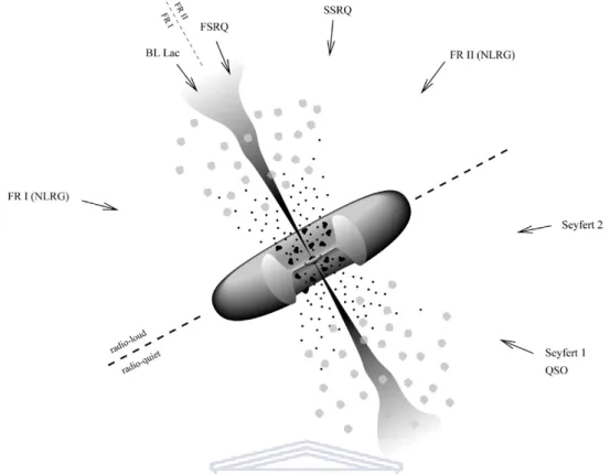
Figure 1.3: The unified model of AGN which explains the types of AGN by different observation

angles. The arrows represent the observation angle, with respect to the jets, to observe a specific AGN type. Blazars Lacertae (BL Lac) and flat-spectrum radio quasars (FSRQ) have an unobscured view of the central region while steep spectrum radio quasars (SSRQ) and Fanaroff and Riley (FR:

Fanaroff and Riley [1974]) narrow-Line Radio galaxies (NLRG) are obscured by the torus. On the radio quiet side, Seyfert 2 galaxies have a more edge-on view than Seyfert 1 and radio-quiet quasars

(QSO). Adapted fromUrry and Padovani[1995];Padovani et al.[1997]

1.2

Galactic processes

Galaxies are observed with different shapes and sizes, ranging from giant spherical blobs of red stars (elliptical) to disk galaxies with well-arranged gas and stars (spirals). These features have been ob-served since 1845 when William Parsons recorded a spiral structure in what was then known as a nebula within the Milky Way. Hubble [1925] proved that some of these nebulae are galaxies in their own right that came with a large variety of morphologies, which led to the first classification scheme known as Hubble’s Tuning Fork (Hubble et al. [1936]).

The different shapes and sizes of galaxies result from interaction with each other gravitationally, through collisions and mergers or lack thereof. The exchange of material during this interaction influences the physical processes (star formation, AGN accretion and feedback), which in turn influence the properties of the galaxy.

1.2.1 Star formation

Star formation (SF) is a process where stars form from the collapse of a giant molecular cloud. The molecular clouds are self-gravitating regions mostly made up of hydrogen (H2) and Carbon monoxide

(CO). A typical cloud has a mass of ≈ 105−6M and average densities of ≈ 102 cm−3 (Williams et al.[2000]). Star formation occurs when some external stimulus causes instability in a smaller clump within the molecular cloud, which leads to the collapse of the clump under its own weight as it collapses the central temperature increases. The clump splits into smaller fragments, which also individually continue to collapse until the central regions of the fragments reach the required temperature needed to ignite nuclear fusion. The fusion generates outward (radiation) pressure that balances the gravitation force. The newly-born stars send winds and shock waves to the surrounding gas, which can prevent SF (negative feedback) or stimulate SF (positive feedback). Stars form according to the initial mass function (Elmegreen [1997]), whereby lower mass stars are more likely to form than their high-mass counterparts. The death of these high-mass stars usually results in a core collapse supernovae explo-sion, which sends shock waves to the surrounding gas (supernovae feedback).

The star formation rate (SFR) of a galaxy quantifies the average rate at which stars form in the galaxy, measured in solar masses per year (Myr−1). The SFR depends on the amount of molecular gas avail-able as well as other processes that affect the gas (feedback and AGN accretion). The availability of large multi-wavelength data from various surveys has allowed for detailed studies of the phases and processes that lead to individual star formation as well as measurements of star-formation rates out to high redshifts (Dunne et al. [2009]; Karim et al. [2011],Zwart et al. [2014]). A typical galaxy such as the Milky Way has a SFR of 1 M yr−1, there are galaxies that have a low SFR and those that undergo an extremely high SFR > 1000M yr−1. A typical galaxy type that has a low SFR is the old dead Ellipticals which mostly contain old stars with very little gas. Galaxies that have extremely high SFR are known as starbursting galaxies, which is a short-lived phase of a galaxy which is usually triggered by mergers or other forms of gravitational interaction with nearby galaxies.

Measuring the star-formation (SF) history of galaxies is important for understanding galaxy evolution; it allows measurements of the growth of stellar mass, and it allows measurements of supernova rates and can constrain cosmological parameters (see e.g.Karim et al. [2011] for an overview). SF leads to radio emission and there is a tight relation between SFR and the radio luminosity.

1.2.2 Active galactic nuclei

Recent studies have shown that local massive galaxies all contain a super-massive black hole (SMBH) at their centres (e.g.Tanaka et al.[1995]). An active galactic nuclei (AGN) is the central region of an

Figure 1.4: (a) shows the FRI radio galaxy 3C 296 (Leahy and Perley[1991]) and (b) shows the FRII radio galaxy Cygnus A Perley et al. [1984]. In both panels the contours represent the surface

brightness (Hardcastle [2005]).

active galaxy (i.e one where matter is accreted onto the SMBH). The sources of radiation from an AGN are: (i) a fraction of the potential and kinetic energy of falling matter are converted into radiation, (ii) synchrotron radiation (Section1.2.4) from the material in the jets and (iv) free-free (Bremsstrahlung) emission from accelerating/decelerating particles in the jets. Without gas to accrete, an AGN would shut down; for this reason, AGNs are usually found in galaxies with young stellar populations (more gas; Schawinski et al.[2009]) and typical have life span of≈108yr (Woltjer [1959]).

A typical picture of a (radio-loud) AGN includes an accretion disk surrounded by a thick dusty torus in the plane of the accretion flow and collimated jets of relativistic particles along the poles of the torus (Fig.1.3). It is well established that the appearance of an AGN depends on the observing angle instead of underlying physical properties (Urry and Padovani[1995]). AGN are divided into two main types, type I and type II. Type I AGN are those seen from the line-of-sight of the black hole (i.e. unobscured) and contain broad emission lines produced by gas rapidly rotating around the black hole (denoted by the dark blobs in Fig. 1.3). Type II AGN are orientated so that the torus obscures the central black hole; these have narrow emission lines from the gas further away from the centre rotating less rapidly (Peterson[1997]).

Fig. 1.3 also shows AGN division related to the radio loudness. Radio-loud AGN have greater radio luminosities than radio-quiet (the technical definitions is given in Section 1.3). The old unification model claimed that radio-loud and radio-quiet AGN have similar processes just viewed from a different angle (e.g.Urry and Padovani [1995]; Fanidakis et al. [2011]). Some authors also claimed that radio-quiet AGNs are just scaled-down versions of radio-loud AGNs (e.g. Ulvestad et al.[2005]). However; they are essentially two different objects; radio-loud AGNs are mainly powered by synchrotron emis-sion in the jets and radio-quiet AGN are mainly powered by SF (e.g.Padovani et al. [2011] Kimball

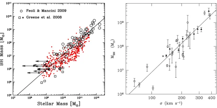
Figure 1.5: (left) The correlation between total stellar mass in the bulge and the mass of the black

hole (BH mass). The red dots are from a simulation byJahnke and Macci`o[2011]; the open circles and triangles are observed data fromFeoli and Mancini[2009] andGreene et al.[2008] respectively. (right) The black hole mass and dispersion velocity (σ) correlation, adapted fromKormendy and Richstone

[1995].

et al. [2011b] ; Condon et al. [2013]) and radiation related directly or indirectly to AGN accretion (e.g. Gruppioni et al. [2003]; Jarvis and Rawlings[2004]). Radio-loud AGN are common in ellipticals and radio-quiet are common in SF spiral hosts (Dunlop et al.[2003]). Furthermore, radio-loud AGNs are thought to contain a binary SMBH system while radio-quiet have a normal SMBH (e.g. Sillanp¨a¨a [1999]).

The final division considered in Fig. 1.3is associated with the FR type I and type II classification by Fanaroff and Riley [1974]. FRI are galaxies with symmetric radio jets with most of their luminosity concentrated in the centre. FRII galaxies are more luminous than FRI, they have jets with lobes that contains bright hotspots at the end (Fig. 1.4).

1.2.3 Feedback

Studies on local galaxies have shown an interesting correlation between the mass of a SMBH and the total stellar mass of the bulge (Fig. 1.5a; e.g. Tremaine et al.[2002]) and an even tighter correlation between the SMBH mass and the stellar bulges’ velocity dispersion (Fig. 1.5b; e.g. Gebhardt et al. [2000], Ferrarese and Merritt [2000]). These correlations suggest that there is a connection between the formation and evolution of SMBH and the bulge (Gebhardt et al.[2000]).Chen et al.[2013] found

a correlation between SFR and the black-hole accretion rate (linked by feedback).

Feedback is a process that regulates the growth of a galaxy, positive feedback leads to growth and negative feedback suppresses growth. There are various types of feedback process, the main ones being SN feedback and AGN feedback. SN feedback occurs when a supernovae goes off and sends shock waves and energy to the intergalactic medium (IGM). This can lead to growth (positive feedback) when the shock waves triggers a collapse of a cloud in the IGM and it can also lead to negative feedback when the energy released heats up the IGM, suppressing star formation (e.g. Best [2007]). AGN feedback is in the form of radio jets. Negative feedback is when the IGM is heated by the radiation from jets and gas is expelled from the galaxy (the expelled gas could have fuelled the AGN (e.g.Morganti et al. [2013]) or collapsed to form stars is expelled and the heated gas suppresses star formation). Silk[2013] claiming that jets can initiate SF by stimulating the collapse of a molecular cloud (positive feedback). Further observational evidence of positive feedback in high-redshift quasars is shown by Kalfountzou et al. [2014].

1.2.4 Synchrotron radiation

Synchrotron radiation is the emission produced when charged particles gyrate in a magnetic field with relativistic velocities (Elder et al.[1947]). The frequency of the radiation depends on the strength of the magnetic field and the velocity of the charged particles. The spectrum from charged particles is due to those electrons gyrating at the fundamental frequency as well as its harmonics (which are closely spaced), making the emission continuous (Grishanin et al. [1991]). The radiation is observed to be linearly polarized when the line-of-sight is perpendicular to the magnetic field, circularly polarized the line-of-sight parallel to the magnetic field and elliptically polarized when the line-of-side is in between perpendicular and parallel. This process is common in astronomical environments and is responsible for radio emission from jets in AGN, galaxies and supernova remnants.

Synchrotron emission is the dominant source of radiation in star-forming galaxies from the super-nova shock of young high-mass stars, which amplifies the magnetic fields and accelerates electrons to relativistic velocities. It is also the main source of radio emission in AGN.

1.2.5 Far-Infrared Radio correlation

There is a known correlation between far-infrared (FIR) emission and radio emission found in local star-forming galaxies (Helou et al. [1985]), which holds over four orders of magnitude in luminosity (Condon et al. [1992]). The FIR radiation is produced when dust absorbs ultraviolet (UV) photons from young massive stars (that ends their lives with a supernovae explosion) and thermally re-emits

in the FIR. The supernova emits both UV radiation and synchrotron radiation, thus, they both trace the SFR of massive stars. The advantage of this correlation is that radio, unlike optical and UV, is not obscured by dust and has higher angular resolution reducing confusion. The correlation holds to high redshifts (z >2) without evolving (e.g. Carilli et al.[2000], Sargent et al. [2010]). However, like with many tracers, there is contamination from synchrotron emission produced by AGN.

1.3

Radio sources

Extragalactic radio sources can be divided into two populations as mentioned earlier; radio-loud and radio-quiet. Radio-loud sources are defined to have radio luminosities above a chosen boundary (e.g. log₁₀[L8.4GHz WHz−1] > 25 (Hooper et al. [1996]). A better measure of radio loudness is defined

by the ratio of the optical and radio luminosities (Schmidt [1970]). Kellermann et al. [1989] used luminosity from 5 GHz in the radio and from B-band (4400˚A) in the optical, defining radio-loudness as an radio-to-optical ratio > 10. At a frequency of 1.4 GHz, radio-loud sources mostly have flux densities above 1 mJy, below which radio-quiet sources start to dominate. Some authors argue that the division between radio-loud and radio-quiet is a result from optical selections, claiming that the radio luminosity of AGN to be continuous (Lacy et al.[2001]).

1.3.1 Radio-loud

Radio-loud sources consist of mostly all the radio-loud AGN; Quasars, FRI, FRII, radio galaxies and blazars, making up only ≈ 10% of the known sample of AGNs. These are all extremely luminous AGNs with typical luminosities log₁₀[L1.4GHz WHz−1] ≈ 24, spanning several orders of magnitude.

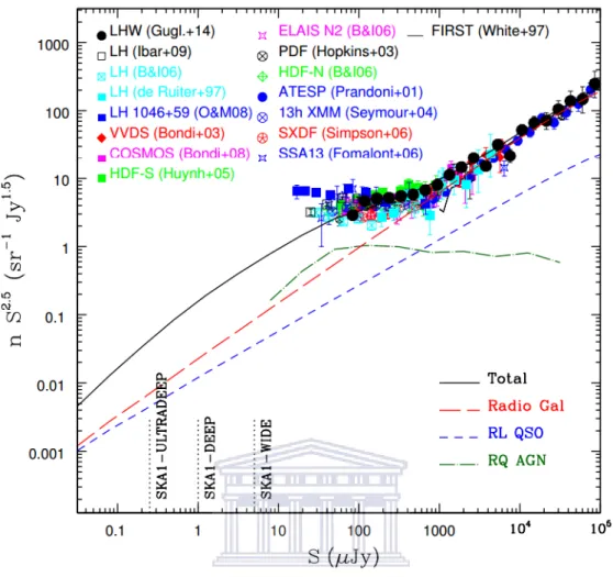
Fig. 1.6 shows that these sources dominate counts from flux densities > 1 mJy and peak at 1 Jy at 1.4 GHz (e.gMitchell and Condon [1985]; Condon et al.[2012]). Numerous multi-wavelength studies of these objects have been conducted since their discovery in the 1940s, but there is a great deal of the processes that are not well understood (e.g. how jets are formed or why certain AGN do not have them).

1.3.2 Radio-quiet

Radio-quiet sources have fainter radio luminosities (and smaller radio-to-optical ratio<10) than the radio-loud sources. At 1.4 GHz, radio-quiet sources dominate the counts at<1 mJy (Fig.1.6). These sources are mainly powered by synchrotron emission from SF; in fact until recently it was thought that SF was the only source of radiation at these fluxes. However, authors argued that (both radio-loud and radio-quiet) AGN have an important contribution to the<1 mJy flux densities ( e.g. Gruppioni et al. [2003], Jarvis and Rawlings[2004], Padovani et al. [2011], [2014], Norris et al. [2013]). Observations

Figure 1.6: The observed 1.4 GHz source counts and simulated counts from various authors (de

Ruiter et al. [1997]; White et al. [1997]; Prandoni et al. [2001]; Hopkins et al. [2003]; Bondi et al.

[2003]; 2008; Seymour et al. [2004]; Huynh et al. [2005]; Biggs and Ivison [2006]; Fomalont et al.

[2006];Simpson et al. [2006];Owen and Morrison[2008]; Ibar et al.[2009];Guglielmino et al. [2014]). The simulated counts are taken from the SKADS model (Wilman et al.[2008];2010) and are divided into Radio galaxies, radio-loud quasars and radio-quiet AGN. The 5σlimits of SKA1 wide, deep and

ultradeep surveys are also shown.

(e.g. Padovani et al. [2014]) show that AGN make up≈40% and radio-quiet AGN make up ≈25% .

Studying radio-quiet AGNs is rather important as they make up a large fraction of the AGN pop-ulation. They can, therefore, help shed light on the mysteries of AGN and galaxy evolution; for example understanding the interaction between AGN feedback and SF (plus they are associated with SF galaxies).

1.4

Quasars

Quasi-stellar radio sources (quasars) are a subset of the AGN population, discovered (Hazard et al. [1963]; Schmidt[1963],Oke [1963]) in the radio as bright point sources with star-like counterparts in

the optical. Their star-like appearance made them indistinguishable from stars, but they have a broad emission spectrum different from any star (Schmidt[1963]). They were found to be galaxies at high redshifts (assuming their redshifts are cosmological).

Quasars are one of the best sources for studying the evolution of the Universe, SF history and AGNs. This is because they are among the brightest objects in the Universe, they are a member of the AGN family, and they span a large redshift range toz≈7 (e.g. Momjian et al.[2014]). Another interesting property of quasars is the unique emission that ranges from UV to x-ray which has been observed at all redshifts (Fan et al.[2004]; Shemmer et al. [2006]; De Rosa et al.[2011]), suggesting that quasars established their nature in the early Universe (Momjian et al.[2014]). However there are a few changes in quasar characteristics with redshift; (i) emission from hot dust (≈ 1000 K) has been observed in low-redshift quasars (Jiang et al. [2010]), (ii) there is a possible decrease in the relative fraction be-tween radio-loud and radio-quiet AGN at high redshifts, which could mean a change in the accretion modes and BH spin of the first quasars (e.g. Dotti et al.[2013]).

Quasars, being AGNs, inherit the uncertainty in their dominant source of radio emission for<1 mJy sources (Fig. 1.6). Recent studies of optically-selected quasars suggest that these sources are domi-nated by SF (Kimball et al.[2011a] andCondon et al.[2013]). However,White et al.[2015] used deeper optical and near-infrared selection of quasars and they suggest that the radio emission is dominated by AGN accretion. The investigation was extended to infrared where Rosario et al. [2013]; showed that infrared emission from radio-quiet low luminosity AGN correlates with star formation and hence the radio emission as well (FIR-radio correlation; Section1.2.5) (Bonzini et al.[2015];Padovani et al. [2015]). However, Zakamska et al. [2016] extended the analysis of Rosario et al. [2013] to two orders of magnitude of luminosity and found the emission is more likely associated with accretion (Lal and Ho [2010]; Harrison et al. [2014]).

Although quasars were first discovered in the radio,Sandage [1965] found that quasars can be identi-fied solely through their optical emission as they have a unique spectrum that is different from stars. Since then quasar were mostly discovered through the use of optical surveys.

A large sample of quasars is needed to resolve the ongoing debates about AGN and quasar emissions. However, quasars are hard to find and thus require large surveys like the Large Bright Quasar Sur-vey (LBQS; Morris et al. [1991]) the 2dF Quasar Redshift Survey (2QZ; Boyle et al. [2000]) and the successive releases of the Sloan Digital Sky Survey (SDSS; York et al. [2000]) quasar catalogues are needed to representative samples. Optically selected quasars suffer from various selection effects: (i) misses reddened quasars which are observed in radio (e.g. Webster et al.[1995];Gregg et al.[2002];Holt et al. [2004]; Glikman et al. [2007]Urrutia et al. [2009] thought to be heavily obscured by dust (e.g.

Richards et al.[2003]; Young et al.[2008]). (ii) Quasars in the redshift range 2< z <3.5 have similar optical colours to stars (e.g. Fan[1999]).

1.5

Large radio surveys

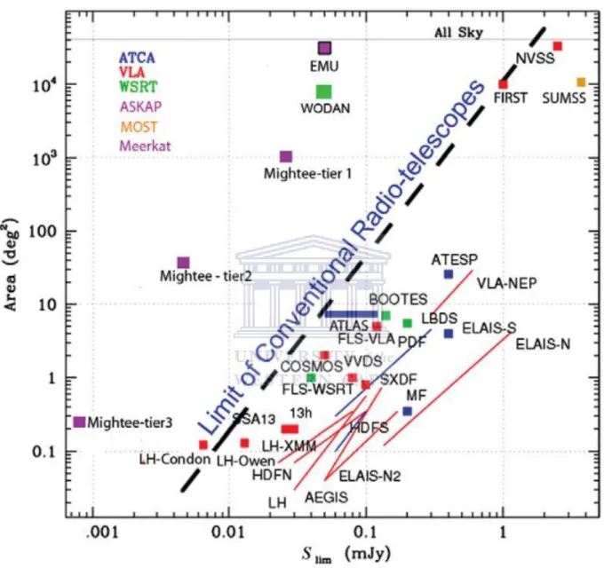
Radio surveys are crucial for studying quasars; because, although AGN typically radiate in a large range of frequencies (including UV, X-ray and optical), radio is where most of the characteristics of AGN are seen (jets and lobes) and where the types of AGN differ the most. Furthermore, the radio does not suffer from obscuration so it is sensitive to all types of AGN irrespective of their orienta-tion. The current regime of large-area radio surveys e.g. the Sydney University Molonglo Sky Survey (SUMSS; Bock et al. [1999]), the NRAO VLA Sky Survey (NVSS; Condon et al. [1998]) and Faint Images of the Radio Sky at Twenty-centimeters (FIRST;Becker et al.[1995]) mostly detect radio-loud sources.

There is a great deal of activity in the development and upgrades of radio telescopes in preparation for the Square Kilometre Array (SKA), which is expected to reach nJy flux levels. The Low-Frequency Radio Array (LOFAR) is complete and in operation. Telescopes that have been upgraded include; the VLA (to the Jansky Very Large Array; JVLA) and MERLIN to e-MERLIN. The telescopes being built include SKA pathfinders like the More Karoo Array Telescope (MeerKAT) and the Australian Square Kilometre Array Pathfinder (ASKAP). These telescopes will survey the sky to fainter fluxes faster than existing telescope (Norris et al.[2013]; Fig. 1.7).

1.6

Outline

This thesis is structured in the following way: In Chapter2, I discuss the optical data from the SDSS and radio data from FIRST. In Chapter3, I use the detected sources to construct source counts and quasar radio luminosity functions and compare to literature. In Chapter4, I explore the fluxes of the sources below the detection using median stacking, which returns a single statistic for a given bin. I take it a step further by constructing the sources counts of the sources below the detection threshold based on fitting a model to the data using a Bayesian approach. In Chapter5I summarise the results found and give future aspects of the work.

Throughout the work unless state otherwise, I use AB magnitudes. All the positions are in J2000 epoch, spectral index α = −0.7 and ΛCDM cosmology, with H0 = 70 km−1 Mpc−1, ΩΛ = 0.7 and

Ωm= 0.3.

Figure 1.7: Next-generation and current radio-continuum surveys at 1.4 GHz. Thex-axis is the 5σ

flux limit, sensitivity increases to the left, and they-axis is the survey area. The diagonal line shows the limit of current telescopes (before upgrades); this is of course mostly limited by telescope observation time, however, in 2016 it would take an unrealistic integration time to cross the line. Credit:,Norris

et al.[2013]        

Chapter 2

Data

For an experiment of this nature where one tries to obtain useful information from sources below the detection limit of a survey, one needs auxiliary data from another survey. I use FIRST radio data with deeper optical data from SDSS that contains fainter sources than First.

2.1

SDSS

The optical sample is drawn from the quasar catalogues of both the twelfth and final data release (DR12) of SDSS III’s BOSS (Eisenstein et al. [2011]) and DR7 of SDSS II’s Legacy (Shen et al. [2011]). SDSS is a spectroscopic redshift survey observed with a dedicated 2.5 metre wide-field (Gunn et al. [2006]) telescope equipped with an multi-band imaging (ugriz (Fukugita et al. [1996]) camera and spectrograph. SDSS started observations in 2000, covering over a third of the sky in various phases with different goals. The survey has gone through three phases, SDSS I, SDSS II, SDSS III and, currently commencing SDSS IV.

2.1.1 SDSS I

SDSS I (York et al. [2000]) was operational until 2005 and imaged over 8,000 square degrees of the sky in five optical bands along with spectroscopic observations of galaxies (Strauss et al.[2002],Eisenstein et al. [2001]) and quasars (Richards et al. [2002]) in what is called the Legacy survey. The quasar targets were observed in a 5,700 square degrees subset of the SDSS I imaging data (top panel of Fig2.1

shows the footprint of these quasars). Legacy found a total of 670,000 galaxies 77,000 quasars.

15      

Figure 2.1: The quasar coverage of all the three phases of the SDSS. The top panel is SDSS I with 77,000 quasars covering an area of 5,700 square degrees, the middle panel is the SDSS II 105,000 quasars found in an area covering 7,500 square degrees. The bottom panel contains 297,301 SDSS III’s

BOSS quasars observed in area covering 10,000 square degrees.q

2.1.2 SDSS II

SDSS II was carried out between 2005 to 2008, completing the Legacy survey and starting both the SEGUE and the Sloan Supernova surveys.

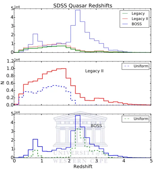
(i) Legacy Surveyprovided uniform coverage in five bands of over 7,500 square degrees of the sky in the North Galactic cap (NGC) and 740 square degrees in the South Galactic cap (SGC). Most of the survey footprint was covered in SDSSI, SDSSI only observed a small part. The complete coverage of Legacy is shown in panel 2 of Fig. 2.1. It containes ≈ 2 million objects, ≈ million galaxy spectra and more than 105,000 quasar spectra. panel 1 of Fig 2.2 shows the redshift distribution (green lines) of the Legacy quasars (Legacy II).

0

1

2

3

4

5

1e4

SDSS Quasar Redshifts

Legacy

Legacy II

BOSS

0.0

0.2

0.4

0.6

0.8

1.0

1.2

N

Legacy II

Uniform

0

1

2

3

4

5

Redshift

0

1

2

3

4

5

BOSS

Uniform

Figure 2.2: The redshift distribution of the SDSS quasars. The top panel is redshift distribution for the three complete phases of the SDSS, SDSS I (Legacy, green line), SDSS II (Legacy II, red line) and SDSS III (BOSS blue line). The redshift distribution of the full Legacy survey (Legacy II, red line) and the uniform subsample (blue dotted lines) are shown in the second panel. The third panel shows

the uniform (green dotted lines) and full BOSS quasars (blue dotted line).

(ii) Sloan Extension for Galactic Understanding and Exploration(SEGUE) was a

spectro-scopic survey of 240,000 stars to study the structure, formation and evolution of the Milky Way (Yanny et al. [2009]).

(iii) The Sloan Supernova surveyis a repeated imaging survey over a 300 square degree area on the Celestial Equator to search for supernovae Ia (Frieman et al. [2008]). The survey ran from 2005 to 2007 and confirmed a total of 327 type Ia supernovae events (Sako[2007]).

2.1.3 SDSS III

SDSS III (Eisenstein et al.[2011]) began operations in 2008 and was completed in 2014. This phase was divided into four different surveys; SEGUE-2, BOSS, APOGEE and MARVELS all conducted with the same 2.5 wide-field Sloan telescope (Gunn et al. [2006]) with the new improvements since SDSS III will observe fainter targets. The improvements include: (i) a multi-object fibre-fed optical spectrographs with new fibres; 1000 fibres with 200apertures per plate instead of the previous 630 fibres with 3” apertures, (ii) new gratings CCDs and optics and (iii) a new near-infrared high-resolution spectrograph and an optical interferometer.

(i) The Sloan Exploration of Galactic Understanding and Evolution 2(SEGUE-2; Rockosi

et al. [2015] in prep.) builds on the work from SEGUE 1. SEGUE 2 spectroscopically observed close to 119,000 unique stars in the halo of the galaxy with distances of 10 to 60 Kpc from the galactic centre. The observations were done over 1317 square degrees from 2008 to 2009.

(ii) Multi-object APO Radial Velocity Exoplanet Large-area Survey (MARVELS; Ge et

al. [2015] in prep.) used two 60-fibre interferometric spectrographs to observe radial properties (e.g velocity) of 11,000 stars in search for exoplanets and brown dwarfs that have orbital periods from several hours to two years. MARVELS operated from 2008 to 2012.

(iii) APO Galactic Evolution Experiment (APOGEE; Majewski et al. [2015] in prep. ) uses a 300-fibre high resolution, high signal-to-noise infrared (H-band) spectrograph to penetrate through the dust that obscures stars, in the galactic disk, bar and bulge and halo, to investigate their dynamics and composition. The data was observed from 2011 to 2014 using stars selected from the 2MASS database.

(iv) Baryon Oscillation Spectroscopic survey(BOSS;Dawson et al.[2013]) used the same imag-ing data as SDSS I and SDSS II, with an additional area in the South Galactic Cap, to a limitimag-ing magnitude of r ' 22.5. BOSS surveyed 7578 deg2 in the NGG and 2663 deg2 in the SGG, a total of 10269 deg2 _{shown in panel 3 of Fig. 2.1. One of BOSS’s key goals is to measure the}

baryon acoustic oscillation (BAO) scale in (i) the distribution of galaxies and neutral hydrogen (Anderson et al. [2014]) and (ii) the Lyman-α forest (Busca et al. [2013]). This is done using spectral information of 1.5 million luminous galaxies brighter than i = 19.9 with z < 0.7 and observations of high-redshift (z >2) quasars (Busca et al.[2013];Slosar et al.[2013];Kirkby and BOSS Collaboration[2013]).

Figure 2.3: A spectrum of a gravitationally-lensed quasar Q1422+231 observed with the HIRES

spectrograph (Vogt [1992]) on the the Keck I telescope. The high redshift quasar is observed at

z= 3.625 and the Lyαforest is located aroundλ∼5000 ˚A, ‘eating every’ (line) feature of the quasar below the Lyαemission, (from Ellison et al.[2000]).

2.1.4 Quasar target selection: SDSS I and II

SDSS I and II targeted objects classified as point-like in the magnitude range 15< i <19.1 (Richards et al. [2002]; 2006). This target selection catches both quasars and stars. Quasars are then differen-tiated from stars by their unique colours in multi-dimensional color-colour space (Fan [1999]). The colours of quasars are reduced by absorption from a phenomenon called Lyα forest (Lynds [1971]). The Lyα forest is a series of Lyα absorption lines, corresponding to the neutral hydrogen transition from n= 1 to n= 2, from foreground intergalactic gas. Due to their large distances, the light from a quasar passes through this intergalactic gas from different redshifts with each leaving its ’mark’ in the spectra of the quasar, resulting in the absorption lines being observed at a range of wavelengths. This phenomenon has a significant effect onz ≥2.2 quasars; Fig 2.3shows the Lyα forest for a z= 3.625 quasar. However, the quasars become reddened with increasing redshift making their colours distinct from stars (Fan[1999], Richards et al. [2001b]). Quasar models by Fan[1999] show that on average quasars are well separated from the stars, with the exception to 2.7 < z < 2.8, where quasars are indistinguishable from A stars and blue horizontal branch (BHB) stars in theu−g,g−rcolour-colour space (Fig2.4). Quasar candidates in SDSS I and II are primary the outliers from the stellar regions in colour-colour space (Richards et al. [2001a]) (as seen in Fig 2.4) and the regions with large stellar contamination were avoided.

As mentioned earlier, one of the main goals of BOSS is to observe BAO scale in the Lyman α forest (Dawson et al. [2013]). This requires spectroscopic detections of 15≥ per quasars deg−2 at z >2.2. To achieve this, they apply a magnitude limit ofg <22 giving a surface density of 20 quasars deg−2at

Figure 2.4: The colour-colour plot (u−g), (g−r) used to identify quasars from various stars. Quasars

(models, Fan [1999]) are shown in different colours according to their redshift, blue representing low redshifts and red high redshifts, and star are represented by black points. The left panel is a subset of the brightest (18< g <19) objects targeted by SDSS I and II, were its one can easily distinction quasars from stars except at 2.7 < z < 2.8. The right panel is a sample of brighter objects (21 < g < 22) targeted by BOSS, which has a lot of contamination from stars due to the large uncertainties in magnitudes because the their are close to SDSS’s photometry limit, (taken fromRoss et al.[2012]).

z >2.2. The magnitude limit is very close to the detection limit of SDSS photometry (Abazajian et al.

[2004]), as a result, it broadens (scatter) the stellar range in colour-colour space (Fig 2.4) therefore increasing contamination. Using the traditional colour-colour space selection will be very challenging as there is contamination from metal-poor A and F stars, faint low redshift quasars (z ≈ 0.8) and compact galaxies which all have the same colours as the target quasars (Richards et al. [2001b]). Therefore, new quasar target selection algorithms had to be developed for BOSS to achieve its goals.

2.1.5 Quasar target selection: SDSS III

Since traditional colour-colour space selection of quasars can not be used, four distinct targeting algorithms are used in SDSS III; the Kernel Density Estimation (KDE;Richards et al.[2004],Richards et al. [2009a]), Likelihoods (Kirkpatrick et al. [2011]), neural network method (Y`eche et al. [2010]) and the Extreme Deconvolution XD (Bovy et al. [2011a],Bovy et al. [2011b]).

(i) Kernel Density(KD) classification scheme was introduced by Gray and Moore [2003], and

Richards et al. [2010] applied the method to SDSS imaging data. The method uses a set of (known) stellar and quasar densities in multi-dimensional colour-colour space, (similar to the left panel of Fig 2.4), as a trained sample. Objects are then given probabilities of being a quasar based on their position colour-colour space with respect to the trained sample.

(ii) The Likelihood method(Kirkpatrick et al.[2011]) uses a similar approach as the KDE method in that it uses a trained set (a model, using all the photometric data and their uncertainties).

The likelihood of an object being a quasar, given its photometric data and errors is the sum of the distance to all the quasars and stars in the trained set in colour-colour space.

(iii) The artificial neural network method (Y`eche et al. [2010]) like the other methods uses a trained set and computes the probability of an object, given all the photometric magnitudes and their uncertainties, is a quasar in the desired redshift (2.15< z <3.5) using four neurons. (iv) The Extreme Deconvolution (XD; Bovy et al. [2011a], Bovy et al. [2011b]) method is a

variation of the Likelihood method that properly accounts for the errors in the magnitudes. XDQSO is an application of XD method to assign a probability of an object being a quasar.

BOSS quasars are divided into several sets; CORE, BONUS, KNOWN, and FIRST with each set having different imaging cuts and flux limits. The cuts and limits were applied to single epoch data except for FIRST targets were co-added, multi-epoch data were used if available (Ross et al. [2012]). Objects with a FIRST flag are thus generally not in the CORE sample.

(i) The CORE quasars are uniformly selected across the BOSS footprint. From the second year to the end of the survey the CORE quasars were identified using the XDQSO target selection method (Bovy et al.[2011b]). During year one, a test year, the KDE selection method (Richards et al. [2004],Richards et al. [2009b]) was used to identify CORE quasars.

(ii) BONUS quasars are selected to maximize the surface density in such that the survey require-ments of 20 ≥ quasars per deg−2 are met. These were selected using a combination of all the target selection methods (KDERichards et al.[2004],Richards et al.[2009b]; likelihood method: Kirkpatrick et al. [2011], neural network, and the XDQSO method (Bovy-2011a) with lower likelihood than in the CORE sample) as well as additional data if needed.

(iii) Objects that have g≤22 orr≤21.85 withFIRST(Becker et al.[1995]) a match within 100 are considered as targets. A additional cut (u−g)>0.4 is applied to exclude low redshift quasars.

(iv) Knownquasars withz >2.15 found in existing catalogues such as DR7 (Schneider et al.[2010]); the 2dF quasar redshift survey (2QZ; Croom et al. [2004]; the 2dF-SDSS LRG, quasar survey (2SLAQ; Croom et al. [2009])); the AAT-UKIDSS-DSS (AUS) survey, the MMT-BOSS pilot survey (Fabricant et al. [2005]) and quasars observed by VLT and KECK, that fall within 1.500 of a point source are considered targets. These are then re-observed to take advantage of the upgraded SDSS spectrograph (Ross et al.[2012]).

2.1.6 Spectroscopy

All the targets from the various selection methods are spectroscopically observed with the BOSS spectrograph. The spectrograph has a metal plate with holes were fibre-optic cables are attached and

Figure 2.5: The left panel shows the geometry of a chunk that contains 47 plates and covers 144 deg2 . The right panel shows the different chunks (each with its own colour coding) that make up the

full BOSS footprintRoss et al. [2012] .

light from a target enters the fibres and are directed to a grism or grating which splits the light to get the spectrum. The holes are distributed such that to maximize the number of the targets observed this is called tilling (the full details of SDSS tiling are found in Blanton et al.[2003]). Due to nature of large-scale and galactic structure, the targets have an inhomogeneous angular density distribution in the sky. Therefore, tilling completeness would mean a non-uniform distribution of the fibre holes. BOSS has a tiling completeness of 93%, this is due to the unobservable regions called masked regions1_.

The are four types of masked regions, bright star mask, central mask, bad field mask and collision priority mask (White et al.[2011]).

(i) Bright star mask

This is the mask that blocks regions around bright stars. The size of the mask depends on the apparent brightness and angular diameter of the star.

(ii) Central mask

The central part of all the plate has a hole for centerpost as a result, targets within a 9200 radius of the central position are removed from the target list.

(iii) Bad field mask

This placed over regions that have bad photometric data.

(iv) Collision priority mask

Two holes in the plate cannot be closer than 6200 in BOSS, this is because fibre optics can not be placed so close to each other and this is known as fibre collision. Collision priority mask is placed around objects that have high priority, so any object that lies within 6200is removed from

1_{www.sdss3.org/dr9/algorithms/boss tiling.php|}

the target list.

The survey is divided into several tilling chunk. A chunk is a set of tiles (might be from a different plate) covering a spatially continuous area observed at the same time and with the same target selec-tion method. Fig2.5ashows the geometry of a chunk within the survey which contains 47 plates and covers 144 square degrees. Fig 2.5b shows the chunks that make up the BOSS survey. Up to 1000 objects can be observed on each plate, with at least three 15 minute exposures or until the required signal to noise is achieved (Pˆaris et al. [2014]).

The geometry of the tilling of BOSS data is expressed in the form of spherical polygons created using the software package Mangle2 (Swanson et al. [2008]). The whole survey is made up of 32,561 polygons of different sizes, to minimize the number of polygons used and to accurately follow the observed regions and avoid the masked regions.

2.1.7 Quasar catalogue

All the spectra of the quasars are visually inspected to ensure that the objects are indeed quasars. Further more identify features in the spectra to confirm or if needed correct the redshift provided by the pipeline (e.g in case a line is misidentified) (Paris et al. [2012]). About 300,000 (297,301) BOSS quasars were spectroscopically identified and released in the twelfth data release (DR12) quasar catalogue of the SDSS III(Pˆaris et al. 2015 in prep).

2.2

Sample

A magnitude limited survey may suffer from various selection effects, for example, Malmquist bias (see Hendry and Simmons[1990]) whereby luminous sources are detected at all redshifts whereas the less luminous sources at high redshifts are not detected. Our quasar sample is taken from the SDSS which has an apparent magnitude limit of r ≈ 22.5 (Dawson et al. [2013]), therefore suffers from the bias. Statistical measurements such as source counts and luminosity functions require uniform and complete data or data that is corrected for biases. I select two samples from the SDSS quasar catalogue to study sources above the FIRST noise (Chapter 3) and a third sample to study sources below FIRST’s detection threshold (Chapter 4). Sample 1 and sample 2 were chosen purely so that the results (source counts and luminosity functions) can be compared with literature (Condon et al. [2013], Kimball et al.[2011a]).

2 http://space.mit.edu/ molly/mangle/|        

2.2.1 Sample 1: Volume-limited sample

The first sample considered is a volume-limited sample. This is a sample where all the sources have an intrinsic brightness above a set minimum. The minimum brightness is chosen such that all the sources that meet these criteria are observed. The sample is chosen in the range 0.2 < z <0.45 and define the volume limit by Mi<−23. Only 162 BOSS quasars fell in the volume-limited sample. I ran into

a problem using BOSS data at these redshifts (because BOSS focused on high redshift quasars, see

2.2.3), so I used SDSS II quasar sample which has 1,313 sources in the redshift range and applied the absolute magnitude limit.

2.2.2 Sample 2: Magnitude-limited sample

The second sample is a magnitude-limited sample. This is a sample where sources have apparent magnitudes above a set value. This kind of sample suffers from Malmquist bias as the sources at different redshifts have different brightness limit. I chose a magnitude limited sample from the redshift range 1.8< z <2.5, favoured in optical quasar samples (e.gCondon et al. [2013];Miller et al. [1990]) because the Lyα line is redshifted into the blue band. The magnitude limited sample is defined by mr < 18, from the 11,613 (29.37%) quasars in this redshift range only 2,419 have the required

magnitudes.

2.2.3 Sample 3: Uniform sample

The third sample is a uniform selection of sources across the survey area (CORE sample). The sample was initially taken solely from BOSS. However, BOSS quasars are not uniformly selected in redshift as it focused on high redshift(and ignored the known low redshift quasarsDawson et al.[2013]).Fig.2.2’s bottom panel shows the redshift distribution of these (BOSS) quasars. The redshift distribution has two peaks, one at z ≈ 2.2 and another at z ≈ 0.8 (Fig 2.2). The quasars around z = 0.8 have the same colours as targeted high redshift quasars (Fig 2.4) and the peak aroundz = 2.2 is a really one showing the underlying distribution of quasars .

The third sample is a combination of Legacy and BOSS. The low redshift part of the sample z <2.15 is from SDSS II’s Legacy quasar catalogue (Shen et al.[2011]) which has an absolute magnitude limit

Mi < −22. Legacy observations from the first data release (DR1) are excluded from the uniform

sample because they were selected using a different algorithm (Shen et al.[2011]). The higher redshift

z > 2.15 sources are from BOSS’s uniform sample defined by Ross et al. [2012], which includes

quasars that have the UNIFORM flag equal one (CORE sample for year 2 onwards) or equal two (CORE sample from year 1). I also apply Legacy’s absolute magnitude cut to the BOSS data so that the whole sample has the same brightness cut. The uniform BOSS sample contains around 122,000

- 5 0 0 5 0 1 0 0 1 5 0 2 0 0 2 5 0 Ra (deg) - 1 0 0 1 0 2 0 3 0 4 0 5 0 6 0 Dec (deg) FIRST Coverage

Figure 2.6: The full 10,575 deg2 footprint of the FIRST maps, divided in two 8,444 deg2 in the

North Galactic Cap (NGC, on the right) and 2,131 deg2 _{in the South Galactic cap (SGC). The SGG}

has rages (holes in the data) due to bad weather and faulty instruments.

sources and the Legacy uniform sample contains around 48,000 sources. Fig.2.8 shows the footprint of the uniform samples.

2.2.4 Completeness

When conducting a survey, one aims to observe all the sources in footprint, however due to certain obstacles, it is not possible. Completeness is a measure of how close the observed sources are to the ‘true’ distribution of the sources (Johnston [2011]). For statistical measurements like source counts and luminosity functions, it is essential to know how many objects are missing. Accurately measuring the completeness is not easy because there are many obstacles to account for. I will divide the sources of incompleteness into two, instrumental obstacles and astronomical obstacles.

(i) Instrumental incompleteness

This is when objects are missed due to technicalities or limitations of the instruments used. This includes sources that missed because they lie in any of the masked regions (Section2.1.6). This source of incompleteness can accounted for by computing the ratio of the sources observed and the target list.

(ii) Astronomical incompleteness

This is when objects are missed because of misclassification or high extinct(McGreer et al.[2009]) or observational biases such as Malmquist bias (Section2.2). It is not trivial to find objects that are misclassified or those that suffer heavy extinction. I correct for Malmquist bias by using volume-limited data.

0.0 0.5 1.0 1.5 2.0 2.5 3.0 FIRST - SDSS sep (arcsec)

0 200 400 600 800 1000 1200 1400 1600 N 4 3 2 1 0 1 2 3 4 ∆RA00 2.0 1.5 1.0 0.5 0.0 0.5 1.0 1.5 2.0 ∆ DEC 00

Figure 2.7: The left panel shows the distribution of the separation between FIRST and SDSS quasar

positions. The vertical dashed line is the cut-off separation between FIRST and SDSS detected sources used in this work. The right panel shows the 2-D scatter of the difference in Right Ascension and

Declination between SDSS and FIRST positions.

2.3

FIRST

The Faint Images of the Radio Sky at Twenty centimeters (FIRST) survey (Becker et al. [1995]) is a high angular resolution survey carried out with the Very large Array (VLA) telescope in its B-configuration at 20 cm (1.4 GHz, L-band). The survey was designed to match the 10,000 deg2 survey area that the SDSS (York et al. [2000]) has covered. Observations started in 1993 and where com-pleted in 2004, additional observations were made in SGC from 2009 to 20113 to observe the ragged portions that were missed due to bad weather or faulty instrumentation. The survey covered a total coverage of 10 575 deg2 with 8 444 deg2 in NGC and 2,131 deg2 in the SGC shown in Fig 2.6. The data is obtained by integrating for 3 min over a pointing on the sky in 7 pair frequency channels centered at 1365 and 1435 MHz. The pointings are designed to produce a uniform sensitivity over the whole survey footprint when all the pointings are co-added (Becker et al. [1995]). Each pointing is reduced (calibrated, self-calibrated, mapped and CLEANed) using an automated AIPS script. The final FIRST maps (Fig 2.6) are obtained by co-adding the individually reduced (weighted) pointings next to each other and stored in binary format as FITS images with 1.800 per pixels having a mean rms of about 150µJy/beam and a 500 resolution (White et al.[1997]).

Sources are identified from the co-added map using HAPPY, a AIPS script (full details are in White et al. [1997]). In brief, HAPPY identifies pixels above a set threshold, appropriately grouping them into ‘islands’ and fitting a two-dimensional Gaussian to each island. Basic properties like peak flux densities, integrated flux densities, right ascension and declination are obtained from this fit. Islands with fitted peak fluxes below 750µJy are removed, the remaining islands are classified and corrected

3_{http://sundog.stsci.edu/first/obsstatus.html}

for the CLEAN bias (White et al.[2007],Condon et al. [1994]) explained in Section 2.5.1.

The survey catalogue contains more than 946,000 sources, over the 10,575 deg2 sky coverage. All sources are above the detection limit, 1 mJy, with an exception of a region in the equatorial strip which contains data from two epochs. As a result, the detection limit is 750µJy, there are ≈ 4,500 sources in this region were the flux densities are below 1 mJy. The catalogue sources have positional accuracies≤100 (White et al. [1997]).

2.4

Matching SDSS with FIRST

2.4.1 Catalogue sources

I am interested in the radio luminosity function of optically selected quasars so I match the SDSS quasars to the FIRST catalogue. A quasar has a match when an object in the FIRST catalogue is found within a certain separation of the SDSS positions. The separation should be as small as possible to avoid random matching with other sources in the FIRST catalogue and it should also be large enough to ensure real matches are not omitted because of slight mismatches in position between the optical and radio data. Fig 2.7 shows the results of the matched sources, the right panel is the distribution of the separation between the matched SDSS and FIRST quasar catalogue positions. The right panel shows the 2-D scatter of the difference in Right Ascension and Declination between SDSS and FIRST positions. The difference in Right Ascension shows a larger scatter compared to the difference in Dec of the sources, this may suggest that the Right Ascension in one or both catalogues is less accurate than the Declination. Fig 2.7suggest a systematic offset on the euclidean separation between FIRST and SDSS catalogues as the peak separation is at 0.200. I choose a limiting separation of 1.800 based on the right panel of Fig 2.7. From the 295,305 quasars, 9,253 (3.13%) matches were found within the limiting separation, 1.800; this is consistent with the low number of optical to radio matches (SDSS to FIRST;Paris et al. [2012]) found.

2.4.2 FIRST cutouts

In the previous section, I matched SDSS quasars to FIRST catalogue sources. However, the catalogue only has sources above the 1 mJy detection limit, which is about 0.02% of the FIRST data (White et al. [2007]) and 3% of the SDSS quasars. Ultimately I am interested in pushing the quasar RLF below the FIRST detection limit to theµJy levels. To do this, I extract a 10-pixel cutout around the SDSS positions From the FIRST maps.

Figure 2.8: The survey footprint of BOSS and Legacy. The area is divided into three regions grey, green and red. The grey region is the part of the sample that falls within the FIRST footprint. The green region is the part of the sample that falls within the FIRST footprint but has zero fluxes and

the red region is the part of the sample that does not fall within FIRST.

265,446 of the BOSS and 101,748 Legacy quasars fall within the FIRST area with a non-zero radio flux (i.e. the data in the region is not corrupted or missing). These sources are represented by the grey region in Fig. 2.8. The quasars in the red region either fall in a region where FIRST has not observed or were observed in bad weather conditions such that the data is corrupted. The quasars in the blue region have zero flux values due to bad data.

2.5

Catalogue and extracted fluxes

The extracted flux density of each quasar is the value of the central pixel of each cutout. The FIRST cutouts contain sources that are detected and sources where there is just noise. It is then important to investigate the difference between the catalogue and extracted fluxes of the detected sources and extrapolate the factors to the sources below the detection threshold that will be used for stacking. The left top panel of Fig2.9is the log-log plot of the peak catalogue fluxes versus the extracted flux. There seems to be a lot of scattering below 10 mJy were the extracted fluxes fall above and below

however most of the extracted fluxes fall below the peak fluxes. Above 10 mJy most of the extracted fluxes are less than the peak fluxes, very few are equal to and even fewer are greater than the peak fluxes. The button left panel shows the fractional difference between the extracted and peak fluxes given by,

fracD = 100×

SX−SP

SP

, (2.1)

where fracD is the fractional difference, SX is the extracted flux and SP is the peak flux. There is

clearly a significant difference between the extracted fluxes and peak fluxes (≈20%) which will have an effect on the results and, therefore, needs to be accounted for or understood. The are two effects considered, the snapshot bias and extraction position.

2.5.1 Snapshot bias

The snapshot bias is an effect that decreases the peak flux densities of detected sources and redistributes it around the field. This phenomenon affects large area radio surveys such as FIRST and NVSS and it is associated with the non-linear CLEAN process (Condon et al. [1994]). The bias is additive and generally constant but the magnitude of the bias depends on (i) the rms of the snapshot (the magnitude increases with noise), (ii) the position with respect to primary beam pattern and (iii) the size of the source (extended sources are affected more) (Condon et al. [1998], Becker et al. [1995]). Furthermore White et al. [2007] discovered that the bias affects sub-threshold sources (which are not CLEANed), suggesting it is associated with the side-lobes of the beam pattern. However, this bias behaves differently from the one associated with CLEAN algorithm as it is multiplicative (the higher the flux the higher the bias). White et al. [2007]’s correction to the snapshot bias (which works for both flavours) is given by

SX = min(1.40SX, SX+ 0.25mJy), (2.2)

whereSX is the extracted flux. The correction was applied to the extracted fluxes and the right panel

of Fig 2.9 shows the results. This correction has a significant effect on the low flux sources and little effect on the high-flux sources. The correction is used for all our extracted data from here on.

2.5.2 Extraction position

The extracted flux densities are from the central pixel of the 10 by 10 FIRST cutout which is centred on the optical position. If the source is not directly at the centre of the cutout, the extracted flux is lower than the detected flux density. The difference in optical and radio positions might be due to the difference the source of radio and optical emission in galaxies. However, because the sources are so far way, this difference is negligible so can not be the source of the difference in radio and optical positions. This difference must be due to astrometry errors between the two surveys.

10-1 ₁₀0 ₁₀1 ₁₀2 ₁₀3 ₁₀4 ₁₀5 Peak flux (mJy)

10-2 10-1 100 101 102 103 104 105

extracted flux (mJy)

Ideal extraction

(a) Extracted fluxes.

10-1 ₁₀0 ₁₀1 ₁₀2 ₁₀3 ₁₀4 ₁₀5 Peak flux (mJy)

10-2 10-1 100 101 102 103 104 105

extracted flux (mJy)

Ideal extraction

(b)bias-corrected fluxes.

100 ₁₀1 ₁₀2 ₁₀3 ₁₀4

Peak flux (mJy)

60 40 20 0 20 40 60 80 100 fractional diff (c)Extracted fluxes. 100 ₁₀1 ₁₀2 ₁₀3 ₁₀4

Peak flux (mJy)

60 40 20 0 20 40 60 80 100 fractional diff (d)bias-corrected fluxes.

Figure 2.9: The difference between FIRST extracted and catalogue fluxes. The top panels is the

plots of the catalogue fluxes versus the extracted fluxes, the solid line represents a case where the extracted flux is equal to the catalogue flux and the red lines are the 5σ. The bottom panels show the fractional difference between the extracted and peak fluxes, described by Eq2.1. The right panels are

corrected for snapshot bias.  

2.6

Sample area

Measuring statistical quantities such as source counts and luminosity functions (LFs) one needs to take into account the sky area in which the sources were observed. Computing this area is not as straightforward as one might think as one cannot simply take the total survey areas of BOSS or Legacy. The area that is required is the overlap between optical and radio surveys shown in Fig2.8, bottom panel for BOSS and middle panel for Legacy.

2.6.1 BOSS overlap

In calculating the overlapping region between BOSS and FIRST I consider the geometry of the BOSS described by different sizes of polygons (see Section2.1.6). I extracted the central coordinates of each of the 32,561 polygons and checked whether it fell in the FIRST coverage. There was one of three situations:

(i) The centre lies within the FIRST maps, then add the area subtended by the polygon to the overlap area. A possible problem arises, does size (of the polygon) matter? I address this below. These fall in the grey regions in Fig 2.8.

(ii) The centre lies within the FIRST maps but the flux is zero. The situation arises when the are no observations in the field but due to the (rectangular) shape of the fits file this region is included or the data is corrupted from bad observing conditions or instrument failure. These fall in the green regions in Fig2.8.

(iii) The last scenario is when the centre does not lie within the FIRST maps. This is when the area was not observed by FIRST and falls in the red regions in Fig 2.8. The results are shown in Fig.5 and Table2.1.

The major flaw of this method is when the size of a polygon is bigger than a 1.800 FIRST pixel. This would mean that there will be an overestimate the area when only a part of the polygon is in FIRST maps (with the centre included) and under-estimate when again a part of the polygon is in FIRST but the centre is not. The polygons are designed to accurately follow the SDSS footprint, so errors are only found in FIRST.

The polygons size ranges from 3.28×10−12 deg2 to 4.11 deg2 and with a median of 0.128 deg2. The FIRST maps have size 1.800 per pixel which corresponds to an area of 2.5×10−7. More than half of the polygons are bigger than the area of a FIRST map pixel

BOSS deg2 Legacy deg2 Total 10269.00 6672.0 Overlap 8609.67 6558.0 Zero flux 304.58 90.0 No-matched 1354.75 24.0

Table 2.1: A summary of the overlap between the two optical samples from BOSS and Legacy surveys

and FIRST maps. Zero flux is the regions of the FIRST maps were no observations were made and the No-matched is the regions that FIRST does not cover.

2.6.2 Legacy overlap

The overlapping area covered by the Legacy is a bigger challenge because unlike with BOSS, polygons describing the geometry are not provided. Legacy only provided coordinates of the spectroscopic plates which project a≈7 deg2 on the sky and unlike polygons, plates overlap with each other. The overlap area is estimated by using a flat sky approximation with 1 deg2 pixels. Then the area is estimated by summing the unique area covered by the projection of the plates that fall in FIRST maps. This method has a lot more uncertainties because the size of the projections is larger than a FIRST pixel. The overlap area between FIRST and Legacy is 6,391.0 deg2_{; the results are shown in Table2.1.}

Chapter 3

Above the detection threshold:

Radio-loud quasars

Before I dive below the detection threshold (≈ 1 mJy), I investigate methods of computing radio source counts and luminosity functions for optically selected quasars detected in FIRST. I will do this for the two samples described in Section2.2, the volume-limited and magnitude samples, and compare my results to the literature.

3.1

Source counts

The simplest and most fundamental experiment one can undertake with objects from a survey is to count their number as a function of flux. Source counts became popular in astronomy whenRyle[1955] and Ryle and Scheuer[1955] found that the 2C survey counts were surprisingly steeper than those of a static uniformly filled Euclidean universe and suggested the radio stars were extragalactic. Longair [1966] then showed the steepening of the counts can be explained by differential cosmic evolution of sources and since then source counts have been used to study extragalactic populations and galaxy evolution (e.g. Rowan-Robinson[1970]; Whittam et al.[2013]).

Source counts are usually presented in differential form n(S)dS, defined as the number of objects per steradian with flux densityS betweenS and S+dS. The integral form of the source counts is defined as the number of sources brighter than flux density S. The integral form is however not favoured as it smoothes out rapid changes of source density with flux density, furthermore, the numbers in each flux density bin are not statistically independent (Jauncey [1967], Crawford et al. [1970]). Even on a logarithmic scale, source counts can be so steep that most of the interesting features are obscured.

33