The University of Manchester Research
Resolved magnetic structures in the disk-halo interface of
NGC 628
DOI:
10.1051/0004-6361/201629907 Document Version
Final published version
Link to publication record in Manchester Research Explorer Citation for published version (APA):
Mulcahy, D., Beck, R., & Heald, G. H. (2017). Resolved magnetic structures in the disk-halo interface of NGC 628.
Astronomy & Astrophysics. https://doi.org/10.1051/0004-6361/201629907
Published in:
Astronomy & Astrophysics Citing this paper
Please note that where the full-text provided on Manchester Research Explorer is the Author Accepted Manuscript or Proof version this may differ from the final Published version. If citing, it is advised that you check and use the publisher's definitive version.
General rights
Copyright and moral rights for the publications made accessible in the Research Explorer are retained by the authors and/or other copyright owners and it is a condition of accessing publications that users recognise and abide by the legal requirements associated with these rights.
Takedown policy
If you believe that this document breaches copyright please refer to the University of Manchester’s Takedown Procedures [http://man.ac.uk/04Y6Bo] or contact [email protected] providing relevant details, so we can investigate your claim.
January 22, 2017
Resolved magnetic structures in the disk-halo interface of NGC 628
D. D. Mulcahy
1?, R. Beck
2, and G. H. Heald
3,4,51 Jodrell Bank Centre for Astrophysics, Alan Turing Building, School of Physics and Astronomy, The University of Manchester, Oxford Road, Manchester, M13 9PL, U.K
2 Max-Planck-Institut für Radioastronomie, Auf dem Hügel 69, 53121 Bonn, Germany
3 CSIRO Astronomy and Space Science, 26 Dick Perry Avenue, Kensington, WA 6151, Australia
4 Netherlands Institute for Radio Astronomy (ASTRON), Postbus 2, 7990 AA Dwingeloo, The Netherlands 5 Kapteyn Astronomical Institute, Postbus 800, 9700 AV Groningen, The Netherlands
Received 14 October 2016/Accepted 21 December 2016
ABSTRACT
Context. Magnetic fields are essential to fully understand the interstellar medium (ISM) and its role in the disk-halo interface of galaxies is still poorly understood. Star formation is known to expel hot gas vertically into the halo and these outflows have important consequences for mean-field dynamo theory in that they can be efficient in removing magnetic helicity.
Aims.We aim to probe the vertical magnetic field and enhance our understanding of the disk-halo interaction of galaxies. Studying a face-on galaxy is essential so that the magnetic field components can be separated in 3D.
Methods. We perform new observations of the nearby face-on spiral galaxy NGC 628 with the Karl G. Jansky Very Large Array (JVLA) at S-band (2.6–3.6 GHz effective bandwidth) and the Effelsberg 100-m telescope at frequencies of 2.6 GHz and 8.35 GHz with a bandwidth of 80 MHz and 1.1 GHz, respectively. Owing to the large bandwidth of the JVLA receiving system, we obtain some of the most sensitive radio continuum images in both total and linearly polarised intensity of any external galaxy observed so far. Results.The application of RM Synthesis to the interferometric polarisation data over this large bandwidth provides high-quality images of Faraday depth and polarisation angle from which we obtained evidence for drivers of magnetic turbulence in the disk-halo connection. Such drivers include a superbubble detected via a significant Faraday depth gradient coinciding with a HIhole. We observe an azimuthal periodic pattern in Faraday depth with a pattern wavelength of 3.7±0.1 kpc, indicating Parker instabilities. The lack of a significant anti-correlation between Faraday depth and magnetic pitch angle indicates that these loops are vertical in nature with little helical twisting, unlike in IC 342. We find that the magnetic pitch angle is systematically larger than the morphological pitch angle of the polarisation arms which gives evidence for the action of a large-scale dynamo where the regular magnetic field is not coupled to the gas flow and obtains a significant radial component. We additionally discover a lone region of ordered magnetic field to the north of the galaxy with a high degree of polarisation and a small pitch angle, a feature that has not been observed in any other galaxy so far and is possibly caused by an asymmetric HIhole.
Conclusions.Until now NGC 628 has been relatively unexplored in radio continuum but with its extended HIdisk and lack of active star formation in its central region has produced a wealth of interesting magnetic phenomena. We observe evidence for two drivers of magnetic turbulence in the disk-halo connection of NGC 628, namely, Parker instabilities and superbubbles.
Key words. ISM: cosmic rays – galaxies: individual: NGC 628 – galaxies: ISM – galaxies: magnetic fields – radio continuum: galaxies
1. Introduction
Understanding of the disk-halo interaction is vital to explain the evolution of spiral galaxies. Several theories exist that describe how star formation expels hot gas vertically into the halo, namely the galactic fountain model (Shapiro & Field 1976; Bregman 1980), the chimney model (Norman & Ikeuchi 1988), and the galactic wind model (Breitschwerdt et al. 1991) relevant to qui-escent star formation (SF), clustered SF and starbursts respec-tively.
These disk-halo outflows have important consequences for mean-field dynamo theory, a process which involves the induc-tive effect of turbulence and differential rotation to amplify the weak magnetic fields to produce strong large-scale fields (Ruz-maikin et al. 1988; Beck et al. 1996). Brandenburg et al. (1995)
? Corresponding author email: [email protected]
Based on observations with the Karl G. Jansky JVLA of the NRAO at Socorro and the 100-m telescope of the Max-Planck-Institut für Ra-dioastronomie at Effelsberg
studied a simple model of such a galactic fountain flow and found that the horizontal field in the galactic disk can be pumped out into the halo to a height of several kpcs. The magnetic field strength at a height of several kpcs was found to be comparable to that in the disk. Mean-field dynamo models including a galac-tic wind may also explain the X-shaped magnegalac-tic fields observed around edge-on galaxies (Moss et al. 2010). Alternatively, sup-pression of the α-effect and of mean-field dynamo action can result from the conservation of magnetic helicity in a medium of high electric conductivity. Shukurov et al. (2006) showed that the galactic fountain flow is efficient in removing magnetic he-licity from galactic disks. This allows the mean magnetic field to saturate at a strength comparable to equipartition with the turbu-lent kinetic energy. However, fast outflows can advect large-scale magnetic fields and hence suppress mean-field dynamo action. As the outflow is expected to be stronger above and below the spiral arms, large-scale fields are weaker than in the inter-arm regions which may explain the observation of magnetic arms be-tween material arms (Chamandy et al. 2015).
Such outflows driven from stellar winds and supernovae from young massive stars in OB associations and super star clus-ters (SSCs) create HI holes (Bagetakos et al. 2011) and
mag-netic field loops pushed up by the gas (Bregman 1980; Nor-man & Ikeuchi 1988). As a result, gradients in Faraday rota-tion measures (RM) and field reversals across these HIholes are
expected. Detecting such RM gradients would constrain the pa-rameters of this outflow model.
Magnetic fields oriented along the disk plane may also bend upwards and become vertical fields as the result of the magnetic Rayleigh-Taylor instability, commonly known as the Parker in-stability. Ionised gas can slide down the magnetic loops, thereby reducing the confining weight of the gas and allowing the loops to rise even higher.
Efforts have been made to observe magnetic field loops. Heald (2012) detected an RM gradient in NGC 6946 across a 600-pc HI hole which indicated a vertical magnetic field.
However, this observational result was obtained for an inclined galaxy, so that the observed RM fluctuations could be affected by the variations of field strengths either parallel or vertical to the disk. Field amplification in the disk can be due to compressive gas motions (density waves) or shearing, while vertical fluctua-tions can be due to Parker loops, which are of kpc scale, or gas outflows. A helically twisted Parker loop was recently found in the spiral galaxy IC 342 (Beck 2015).
Studying a face-on galaxy like NGC 628 is essential so that the magnetic field components can be separated in 3D. In this case, RMs are only sensitive to vertical fields, while synchrotron emission traces the magnetic field in the disk.
NGC 628 = M74 is a large, grand-design, isolated spiral galaxy with a low inclination angle and a HIdisk with a
diame-ter of about 300, about three times the Holmberg diameter
(Kam-phuis & Briggs 1992). A list of physical parameters is given in Table 1. The spiral structure is grand-design but with broad spi-ral arms. The apparent absence of strong density waves is related to the lack of a strong bar or an interacting companion, leaving the disk largely undisturbed (seen in optical, UV, and in gas kine-matics). NGC 628 is similar to NGC 6946 in many respects and hosts many HIholes (Bagetakos et al. 2011). NGC 628 actually
contains nearly twice the number of HIholes (102 holes)
com-pared to NGC 6946 (54 holes) found by Bagetakos et al. (2011), but previous studies performed by Boomsma et al. (2008) found 121 HIholes for NGC 6946 with inferior resolution compared to
Bagetakos et al. (2011).
The high star-formation rate of NGC 628 leads to a bright disk in radio continuum (synchrotron+thermal) of about 100×80
extent (Condon 1987). Marcum et al. (2001) observed NGC 628 extensively in UV. Bright knots embedded in diffuse emission trace the spiral pattern and many of these knots are also bright in Hα(Dale et al. 2009). Marcum et al. (2001) suggested that the entire disk of NGC 628 has undergone active star formation within the past 500 Myr and that the inner regions have experi-enced more rapidly declining star formation than the outer re-gions.
NGC 628 was part of the Westerbork Synthesis Radio Tele-scope (WSRT) SINGS (The SIRTF Nearby Galaxies Survey) survey and was also observed in polarised radio continuum at 1.5 GHz with moderate resolution (Heald et al. 2009). The po-larised emission is restricted to the outer disk and the observed Faraday depths are small, due to strong Faraday depolarisation at this frequency, similar to NGC 6946 observed at the same fre-quency. With the exception of this observation, NGC 628 has not been studied in radio continuum.
Table 1: Physical parameters of NGC 628.
Morphologya SAc
Position of the nucleus RA(J2000)=01h36m41s.74 DEC(J2000)= +15◦47001.100
Position angle of major axisb 20◦
D25a 10.5×9.50
Inclination of the inner diskb 7◦(0◦is face on)
Inclination of the outer diskb 13.5◦
Distancec 7.3 Mpc (100 ≈35 pc)
Star formation rated 1.21 M
yr−1
(a)de Vaucouleurs et al. (1991)(b)Kamphuis & Briggs (1992) (c)Karachentsev et al. (2004)(d)Walter et al. (2008)
Due to its small inclination and large angular size, NGC 628 is one of the best galaxies to study the magnetic field of the disk. However, its low inclination makes it difficult to extract an ac-curate rotation curve and was not computed in the THINGS HI
Nearby Galaxy Survey (de Blok et al. 2008). Kamphuis & Briggs (1992) derived from their HIobservations that the rotation
veloc-ity reaches 200 km s−1.
In this paper, we present new Karl G. Jansky Very Large Ar-ray (JVLA) S-band observations of NGC 628 along with Eff els-berg observations at 2.6 GHz and 8.35 GHz including both total power and polarisation. Sect. 2 presents details of the observa-tions and data reduction, Sect. 3 shows the Effelsberg maps and comparison between the extracted flux densities with literature. In Sect. 4 we present the new JVLA observations, compare to observations at other wavelengths, and determine magnetic field strengths. In Sect. 5 we show results of RM Synthesis in probing the vertical magnetic field of NGC 628. In Sect. 6 we discuss the implications of our main findings and in Sect. 7 we summarise our findings.
2. Observations and data reduction
In this section we describe the nature of the observations taken with the JVLA and Effelsberg 100-metre telescope and the steps performed in the data reduction, starting with the Effelsberg ob-servations. A brief summary of the observational parameters is given in Table 2.
2.1. Effelsberg observations at 2.6 GHz and 8.35 GHz NGC 628 was observed at 2.6 GHz and 8.35 GHz (with band-widths of 80 MHz and 1.1 GHz, respectively) in October 2011 by the authors. The maps were scanned alternating in RA and DEC with the one-horn secondary-focus systems. The data was reduced with the NOD2 software (Haslam 1974). As Radio Frequency Interference (RFI) can be a substantial problem at 8.35 GHz, NGC 628 was only observed at higher elevations at this frequency. 4 out of 32 coverages had to be discarded due to extremely bad RFI. NGC 628 was observed at 2.6 GHz at lower elevations as the RFI is not as severe at this frequency. However, significant RFI was still present and had to be flagged in Stokes I, Q, & U. The final Effelsberg images at 2.6 GHz and 8.35 GHz were obtained from 13 and 28 coverages, respectively, and com-bined using the spatial-frequency weighting method of Emerson & Gräve (1988).
A flux density scaling was applied to the 8.35 GHz data using maps of two calibrators, 3C286 and 3C48. Using values from the
Table 2: Radio continuum observational parameters of NGC 628.
JVLA Effelsberg
Frequency (GHz) 2-4 2.6 & 8.35
Bandwidth (MHz) 2000 (of which 1000 are useful) 80 & 1100
No. of spectral windows 16 –
Total no. of channels 1024 8 & 1
Array configuration D; C –
Pointings 7 –
Observing dates March & July 2013, respectively October 2011
VLA calibrator handbook1, a common scale factor was found and was applied to the target data. For both calibrators, the lin-early polarised intensity and polarisation angle were found by fitting a 2D-Gaussian over the Stokes Q & U maps and calcu-lated from the following equations:
Plin=
q
U2+Q2−(1.2σ
QU)2 (1)
whereσis the noise in Stokes Q and U,
φ=1
2arctan( U
Q). (2)
From the seven maps of 3C48, one had a very different value for the polarisation angle and was discarded. The remaining maps gave a degree of polarisation of 5.5% and a polarisation angle of −65◦. This agrees very well with the values of 5.3% and−64◦for 8.1 GHz found by Perley & Butler (2013b). In
ad-dition, for two maps of 3C286, the degree of polarisation was 11.65% and the polarisation angle was 33.8◦. Again, this is in
excellent agreement to Perley & Butler (2013b) who found val-ues of 11.7% and 33◦. Therefore, we can be confident that the
polarisation calibration for our target is accurate. The level of instrumental polarisation is below 1% at both frequencies.
As the 2.6 GHz receiver is equipped with a 8 channel po-larimeter, an additional bandwidth calibration had to be per-formed along with the normal flux density scaling. For each of the eight channels, the flux density of the calibrator 3C295 was compared to its theoretical value, using a power law with a spec-tral index of -1.04. A scale factor was then determined from the ratio of the two and applied to each channel. The final images for both frequencies are presented in Figures 1 & 2.
2.2. JVLA observations at S-band
NGC 628 was observed by the JVLA in D and C configurations in February and June 2013 in S-band (2–4 GHz). The synthe-sised beamwidth for a 12 hour observation with uniform weight-ing scheme is approximately 2300 for D configuration at 3 GHz and 7.000 for C configuration. The ultimate factor limiting the
field of view is the diffraction-limited response of the individual antennas.
An approximate formula for the full width at half power (FWHM) of the primary beam (in arcminutes) is: FWHM = 450/νGHz. For the highest frequency (4 GHz) in S-band, FWHM
is approximately 100.
As NGC 628 is extended over 10.50in angular size (Table 1),
observations with several pointings were needed.
For this purpose, a hexagonal grid was chosen for both D and C configurations consisting of 7 pointings, separated by 50.
1 http://www.aoc.nrao.edu/gtaylor/csource.html
While the pointing grid is oversampled, this is a safe approach as every position in the galaxy is at least covered three times. In ad-dition, this makes the observations more sensitive to NGC 628’s extended disk.
S-band is subject to very strong RFI from a number of lites in particular those providing satellite radio service. A satel-lite passing through the initial slew will cause unwanted erro-neous attenuator settings. Therefore, in order to prevent this, the observation was started with a quick L-band scan on 3C48 which was in a satellite free zone at this time. After this, the S-band was switched on.
3C48 was observed at the start of the observation so it could be used as the main flux density calibrator to calibrate band-pass and absolute flux densities. The source J0240+1848 was ob-served at least once per hour for use as a phase and polarisation leakage calibrator. 3C138 was observed twice during the obser-vation in order to calibrate the polarisation angle. Between these calibrator scans, all 7 pointings of the NGC 628 were performed several times. The D & C configuration observations were a total of 5 & 6 hours long.
2.3. Calibration of JVLA S-band data
The data were reduced using the Common Astronomy Software Applications (CASA) package2(McMullin et al. 2007). Both D
and C configurations were calibrated identically but separately. Data affected by shadowed antennas were flagged. As RFI can be extremely strong in S-band and as this RFI can produce sharp edges in the spectrum, this can introduce an oscillation across the frequency channels where no RFI is present. This is called Gibbs’ phenomenon and can be brought under control by using Hanning smoothing. Due to extreme RFI in several spec-tral windows at the two extremities of S-band, the bandwidths 2.0–2.6 GHz and 3.6–4 GHz were completely flagged. The re-sulting central frequency is 3.1 GHz.
A table of antenna position corrections was produced and in-corporated into our calibration using the task GENCAL. A pre-liminary bandpass correction was applied to the data in order to maximise the effectiveness of the automatic flagging. Visibilities affected by RFI were flagged via the automatic flagging routine RFLAG. The antenna EA21 was flagged due to higher than av-erage amplitudes.
The model of 3C48 was taken from Perley & Butler (2013a) and was used as our main flux density and bandpass calibrator. The residual delays of each antenna relative to the reference an-tenna were found using 3C48. The delays for all anan-tennas were seen to be on average approximately 4 ns and none were greater than 8 ns. Next, the corrections for the complex antenna gains were obtained. The gain amplitudes were determined by refer-encing our standard flux density calibrator. To determine the
Table 3: Imaging parameters of the NGC 628 JVLA data. Natural weighting
Angular resolution 1800(630 pc)
Cell size 300
Min & max cleaning scales 3.000 18000
Robust weighting (0.0)
Angular resolution 7.500(265 pc)
Cell size 1.500
Min & max cleaning scales 1.500 18000
propriate complex gains for the target source, we used our phase calibrator, J0240+1848. This was the closest and most appropri-ate phase calibrator that could be found to our target in order to minimise the differences through the ionosphere and troposphere between the phase calibrator and the target source.
For polarisation calibration, the cross-hand delays due to the residual difference between the R and L correlations on the refer-ence antenna were solved using 3C138 which has a higher polar-isation signal than 3C48. Prior to this, the Q and U values were assigned to 3C138 using the model of Perley & Butler (2013b).
The phase calibrator (J0240+1848) had sufficient parallactic coverage for both observations and was used to solve for polari-sation leakage (usually 5%).
3C138 was then used to solve for the polarisation angle. Once this was done, all calibration tables were applied to the calibrators and each pointing for the target. The C and D config-urations were combined in order to increase the signal-to-noise ratio and maximise the combined uv coverage of the observation. Self-calibration was tested on the target, however the result-ing gain solutions were poor. Applyresult-ing these solutions degraded the image which was most likely caused by the low signal-to-noise ratio and diffuse nature of this particular target. Therefore, self-calibration was not performed.
2.4. Imaging and mosaicing
The Clark CLEAN algorithm (Clark 1980) was used to decon-volve the dirty beam (point spread function; PSF) from the dirty map.
The best strategy found for cleaning the naturally weighted images was to perform CLEAN using a mask until all residu-als are cleaned, followed by 20,000 clean iterations without a mask and without multi-scale CLEAN. In order to model the ex-tended emission in the field of view, multi-scale CLEAN (Corn-well 2008) was performed with scales ranging from 1.500 to
18000. A summary of the imaging parameters is given in
Ta-ble 3. Multi-scale CLEAN is an extension to CLEAN that mod-els the sky brightness by the summation of components of emis-sion having different size scales. The noise for each pointing was found on average to be 5.1µJy/beam for natural weighting and 6.9µJy/beam for robust weighting on average for total intensity (beam sizes can be seen in Table 3). For Stokes Q & U, the noise was found to be approximately 4.5µJy/beam and 6.5µJy/beam for natural and robust weighting, respectively.
Multi-frequency synthesis (Rau & Cornwell 2011) was at-tempted with the Taylor terms set to 2. However, it was found that the very weak diffuse emission to the north of the galaxy would be degraded. Leaving the Taylor terms set to 1 was found to produce far better results for this weak extended emission. Unfortunately this means that we are not able to estimate the in-band spectral index, Condon (2015) states that the in-band
spectral index for JVLA S-band is only reliable for very strong compact sources with a signal-to-noise ratio of≈50; in addition, the apparent spectral indices of extended sources would be too steep as the synthesised beam solid angle decreases by a factor of four across the S-band. In our case, NGC 628 is too weak, dif-fuse and extended for the in-band spectral index to be reliable.
Each of the seven pointings was imaged separately for each Stokes parameter and then mosaiced together. The primary beam of the final image was constructed from each pointing and ap-plied to the final image. The final image of NGC 628 in total intensity at 7.500resolution is shown in Fig. 4.
3. Results from Effelsberg data
3.1. Effelsberg maps
The final images of NGC 628 observed with the Effelsberg tele-scope are shown in Figures 1 & 2. The rms noise for total inten-sity at 8.35 GHz and 2.6 GHz were found to be 0.28 mJy/beam and 1.1 mJy/beam with their resolutions being 8100and 4.60. The average rms noise for Stokes Q and U for 8.35 GHz and 2.6 GHz were found to be 0.10 mJy/beam & 0.30 mJy/beam, respectively. At 8.35 GHz, NGC 628 is found to be very asymmetric. The most intense emission is seen to the north of the galaxy, at RA(J2000)=01h 36m41s, DEC(J2000)= +15◦4802900 rather
than the centre of the galaxy, suggesting that NGC 628 does not have an active nucleus like M 51 (Rampadarath et al. 2015). The brightest region of NGC 628 is part of the northern spiral arm, consisting of many HIIregions, and is also bright in the infrared
spectral range (Kennicutt et al. 2011) and in HI line emission
(Walter et al. 2008). This agrees with the observation of Marcum et al. (2001) that the inner regions of the galaxy have experienced more rapidly declining star formation than the outer regions.
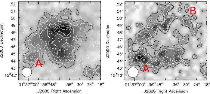
In linear polarisation, the 8.35 GHz map shows diffuse emis-sion along with the polarisation angles forming a spiral pat-tern. A polarised background source (J013657+154422, shown with the letter A in Fig. 1) is apparent at the south-east of the galaxy. There is no sign of polarisation in the central region of the galaxy, probably due to beam depolarisation.
On the 2.6 GHz map, no significant features can be made out in total intensity, owing to the poor resolution of the Ef-felsberg telescope at this frequency. The total intensity emission is seen to extend to the southwest due to an unresolved back-ground source (seen as the letter C in Fig. 2 and 4). Significant polarisation is detected, with the polarisation angles creating a spiral pattern. No polarisation can be seen in the central region. The strongest polarised emission is seen again at the location of J013657+154422 (letter A in Fig. 2 (right)) but significant dif-fuse polarised emission is also observed. Most likely this emis-sion originates from the inter-arm regions of NGC 628 which will be become apparent when inspecting the JVLA data.
3.2. Integrated radio continuum spectral analysis
The integrated flux densities found for NGC 628 are 38±3 mJy at 8.35 GHz and 110±10 mJy at 2.6 GHz. Measurements from the literature (Table 4) were also used to determine the spectral index of the galaxy. All these measurements are tied to the flux scale of Baars et al. (1977). A single power-law fit to the data yields a spectral index ofα=−0.79±0.06. A plot of this data can be seen in Fig. 3. This value not only agrees with Paladino et al. (2009) (α=−0.78) but is a normal value for spiral galaxies (α=−0.74±0.03, Gioia et al. (1982)).
A
A
B
Fig. 1: NGC 628 observed at 8.35 GHz with the Effelsberg 100-m telescope at a resolution of 8100. The left image displays the total intensity of NGC 628 with contours representing 3, 5, 8, 10, 12, 14, 15×30µJy/beam. The right image displays the linearly polarised intensity of NGC 628 with contours representing 3, 4, 5, 8×60µJy/beam. The vectors show E+90◦, not corrected for Faraday rotation, which is very small at this frequency. All vectors are plotted with the same length.
C
A
Fig. 2: NGC 628 observed at 2.65 GHz with the Effelsberg 100-m telescope at a resolution of 4.60. The left image displays the total intensity of NGC 628 with contours representing 3, 5, 8, 16, 32, 44×1 mJy/beam. The right image displays the linearly polarised intensity of NGC 628 with contours representing 3, 5, 8, 10, 12 ×2.5 mJy/beam. The vectors show E +90◦, not corrected for
Faraday rotation, which is small at this frequency. All vectors are plotted with the same length.
At low frequencies, the spectrum of NGC 628 shows no indi-cations of flattening all the way down to 57 MHz. This suggests that neither free-free absorption of the synchrotron emission nor ionisation losses are significant for the galaxy as a whole. The galaxy’s integrated spectrum remains a power law, probably due to the clumpy nature of the ISM (Basu et al. 2015).
A straight power-law spectrum was also seen for M 51 down to 151 MHz (Mulcahy et al. 2014). It should be noted that the flux density of NGC 628 from Israel & Mahoney (1990) is un-certain due to the poor sensitivity and angular resolution of the
Clark Lake telescope and should be treated cautiously. With-out this integrated flux, the fitted spectral index is found to be
α=−0.79±0.03. Unfortunately, no other integrated fluxes has been taken at these low frequencies. Observations with LOFAR (van Haarlem et al. 2013) below 100 MHz are underway and will help to verify whether the integrated spectrum is indeed a straight power law but will additionally be able to resolve this galaxy to arcsecond resolution.
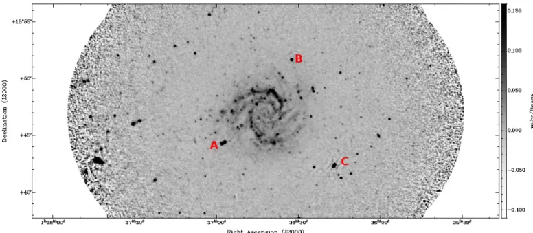
Fig. 4: Total intensity map of NGC 628 at 3.1 GHz at 7.500 resolution, observed with the combined D & C configurations of the JVLA. The rms noise is approximately 5µJy/beam. This image has been primary beam corrected. Several background sources are labeled for future reference.
Table 4: Integrated flux densities of NGC 628.
ν(GHz) Flux density (Jy) Reference
8.35 0.038±0.003 This work 4.85 0.06±0.005 Paladino et al. (2009) 2.614 0.11±0.01 This work 1.515 0.16±0.01 Paladino et al. (2009) 1.4 0.15±0.01 Condon et al. (1998) 0.324 0.49±0.03 Paladino et al. (2009)
0.057 2±1 Israel & Mahoney (1990)
Fig. 3: Integrated spectrum of NGC 628 using Effelsberg and lit-erature integrated flux measurements with the red line represent-ing a srepresent-ingle power law with a spectral index ofα=−0.79±0.06.
4. Results from JVLA S-band data
4.1. Total intensity
The final total intensity image produced with robust weighting at 7.500resolution is shown in Fig. 4, with robust weighting and
smoothed to 1000 resolution in Fig. 5 (upper image), and with
natural weighting at 1800resolution in Fig. 6 (upper image). The integrated flux density of the JVLA data at 3.1 GHz is approximately 120 mJy. This is comparable to the Effelsberg ob-servation at 2.6 GHz (Table 4), demonstrating that the flux den-sity calibration was successful and that there is no significant flux density loss due to the missing small spacings of the JVLA. Weak radio emission surrounds NGC 628 and should be mostly nonthermal in nature (Fig. 6, upper panel). Two main radio spiral arms are present, both coiling out in a counter-clockwise fashion. One spiral arm dominates the north and east of the galaxy (“outer arm”) with the most intense emission lo-cated at RA(J2000)=01h36m38s, DEC(J2000)= +15◦4804700, corresponding to a cluster of HIIregions which are unresolved in
the radio image. This region shows strong emission in Hα (Ken-nicutt et al. 2003) and UV (Marcum et al. 2001), in addition to HI (Walter et al. 2008). The outer arm branches out into two
components in the east (Fig. 5, upper image).
The second main spiral arm (“inner arm”) travels counter-clockwise from north to the south; several HII complexes are
located along the radio spiral arm (Fig. 6, upper panel). These so-called ’beads on a string’ are bright knots embedded in dif-fuse emission tracing the spiral pattern. Many of the UV-bright knots are also bright in Hαindicating recent (less than 100 Myrs) star formation and the radio continuum matches very well to the brightest of these knots. These are especially evident in Fig. 4 where the resolution is high enough to resolve these individ-ual knots. The brightest of these knots are located on the inside edges of the spiral arms formed by the diffuse UV continuum. The youngest and most massive stars are located at the inner edge of the pattern (Chen et al. 1992; Cornett et al. 1994; Mar-cum et al. 2001) which are the knots observed at 3.1 GHz. The inner arm continues to the west where the flux density of the arm suddenly decreases and becomes indistinguishable from the radio envelope of the galaxy, with exception of the HIIregions
located at RA(J2000)=01h 36m29s, DEC(J2000)= +15◦ 480 5000.
Fig. 5: Robust-weighted JVLA image of NGC 628 of total intensity (top) and linearly polarised intensity (bottom) at 3.1 GHz at a
resolution of 1000, averaged over all channels, and overlaid onto an 70µm IR image from Herschel (Kennicutt et al. 2011). Contours
of total intensity are at 1, 2, 3, 4, 6, 8, 12, 16, 32, 64, 128×40µJy/beam. The nonthermal arms to the west are marked Wa to Wc for future reference. Contours of polarised intensity are at 1, 2, 3, 4, 6, 8, 12×12µJy/beam. The white lines show the magnetic field orientations (E+90◦), not corrected for Faraday rotation, with a length of 1000representing 30% degree of polarisation. The main polarised arms are marked from 1 to 3 for future reference.
To the west of the galaxy, three narrow radio filaments are seen (marked Wa,Wb and Wc on Fig. 5, upper image), all with a
Fig. 6: Natural-weighted JVLA image of NGC 628 of total intensity (top) and linearly polarised intensity (bottom) at 3.1 GHz at a resolution of 1800, averaged over all channels. Contours of total intensity are at 1, 2, 4, 8, 12, 16, 32×20µJy/beam. Contours of polarised intensity are at 1, 2, 3, 4, 8, 12×15µJy/beam. The lines show the magnetic field vectors (E+90◦), not corrected for
Faraday rotation, with a length of 1000 representing a polarised intensity of 150µJy/beam (top) and 30% degree of polarisation
(bottom), respectively. The roman numerals I and II refer to the HIholes shown in Fig. 7.
extension of the inner arm. No major HIIregions exist in these
regions and therefore the emission is most likely nonthermal. Unlike most nearby galaxies observed in radio continuum, for example M 51 (Mulcahy et al. 2014), IC 342 (Beck 2015) and NGC 6946 (Beck 2007), NGC 628 shows no trace of a central
source, while this is similar to the flocculent galaxy NGC 4414 (Soida et al. 2002).
4.2. Comparison toHIobservations
Throughout the disk, there are regions where little to no radio emission is seen, most notably the holes located at RA(J2000)
=01h 36m48s, DEC(J2000)= +15◦4501000and RA(J2000)=
01h 36m 50s, DEC(J2000)= +15◦ 460 2700 (shown in Fig. 6 & Fig. 7 as Roman numerials). These holes in radio emission cor-respond to HIholes detected by Bagetakos et al. (2011) (Fig. 7).
Several more holes can be seen in the west of the galaxy. A list of HIholes corresponding to holes in radio continuum and their
physical parameters (from Bagetakos et al. (2011)) is given in Table 5. All the holes seen are of type 1 which is a hole where the gas has been completely blown out of the disk of the galaxy. Approximately 75% of all HIholes are type 1.
Such holes in total radio continuum corresponding to an HI
hole have been seen previously in NGC 6946 by Beck (2007) who mentioned that the association between an HI hole and
radio continuum is rare and that the lack of radio emission could be due to two main reasons. The first is that the super-bubble creating the HIholes, which are driven by multiple
su-pernova explosions, are sweeping away the gas and magnetic field and thereby creating a locally weak magnetic field. The second explanation is that the superbubble carries the magnetic field vertically into the halo along with the hot gas (Norman & Ikeuchi 1988). As NGC 628 is nearly exactly face-on compared to NGC 6946 (i = 33◦), these vertical fields would be along the line of sight, therefore producing no observable synchrotron emission but possibly strong Faraday rotation (see Sect 5.6).
The larger number of HIholes corresponding to holes in the
radio continuum in NGC 628 compared to NGC 6946 could be an effect of the different inclinations. When viewing a HIhole
carrying a magnetic field in NGC 6946 vertical to the disk with its inclination of approximately 33◦, we observe variations of the magnetic field component perpendicular to the line of sight which would give rise to observable synchrotron emission. This would occur less likely for NGC 628 with its smaller inclination. The HIholes seen in NGC 628 all have a kinetic age greater
than 40 Myrs and should be old enough so that the field con-figuration has gained a significant vertical offset (Heald 2012). However, two holes are significantly older and the vertical shear should have destroyed the vertical offset of the magnetic field. Notably, these holes are the most obvious in our radio contin-uum image (Fig. 7). While the vertical shear of NGC 628 is not known to the authors’ knowledge, Heald et al. (2007) found that the vertical shear for a sample of three galaxies is approximately 15–25 km s−1per scale height in Hα, independent of radius. This
gives a lower limit of 60 Myrs for a characteristic shear time. Therefore the first argument is more likely to be true, especially for the two HIholes in question shown in Fig. 7, namely that the
gas and magnetic field have been radially swept away, leaving a weak local magnetic field.
To the north of the galaxy, extended, low-level emission is observed (Fig. 6, top), reaching out to 13 kpc from the centre of the galaxy. The extension is seen to the north–north-west di-rection. Significant HIemission is present in this region and the
radio emission overlays well with the extended northern HIarm
(Fig. 8). Additionally, there are plenty of HIIregions located in
the extended disk of NGC 628. Many of these HII regions are
located on the HI arm (Ferguson et al. 1998; Lelièvre & Roy
2000). HIIregions in the inner disk usually have a star-formation
rate (SFR) of≈103higher than that of the faintest HIIregions in
the outer disk. Therefore, it is most likely that we are observing cosmic ray electrons originating from supernovae occurring at these faint HIIknots from this extreme northern spiral arm.
Fig. 7: Overlay of two prominent HIholes on the radio
contin-uum image (Fig. 5) at 1000 resolution. The contour level is at 21µJy/beam which is approximately 3σ.
Fig. 8: Overlay of the radio continuum emission (red contours) to the north of NGC 628 onto HITHINGS data (greyscale), both
smoothed to the same resolution of 1800. Contours are at 20, 40,
120µJy/beam.
4.3. Separation of thermal emission
For an accurate determination of the magnetic field strength, sep-arating the two components of continuum emission, namely free-free (thermal) and synchrotron (nonthermal) needs to be per-formed. There are several methods, the classical approach where a constant nonthermal spectral index is assumed (e.g. Klein et al. 1984) or using the 24µm infrared emission to directly calcu-late the thermal emission (Murphy et al. 2008). For this work we shall apply the method by Tabatabaei et al. (2007a) where an extinction-corrected Hαmap is used to estimate the thermal emission. The continuum-subtracted Hαmap used was obtained from the ancillary data at the SINGS (Kennicutt et al. 2003) web-site. The maps were in units of DN s−1pixel−1 which was
con-Table 5: List of HIholes corresponding to holes in radio continuum and their physical parameters. tkin, EE & MHIare the kinetic
age, energy requirement, and missing HImass of the HIhole (from Bagetakos et al. (2011)).
RA Dec Diameter tkin log(EE) log(MHI)
(h m s) (◦ 0 00) (pc) (Myrs) (1050ergs) (104M ) 01 36 28.7 +15 46 42.0 878 61 3.0 2.8 01 36 31.1 +15 48 26.9 814 57 2.9 2.7 01 36 31.4 +15 47 20.9 585 41 2.4 2.3 01 36 32.8 +15 47 46.4 901 63 3.0 2.6 01 36 33.2 +15 46 56.8 743 52 2.8 2.5 01 36 35.0 +15 47 20.8 888 62 3.1 2.6 01 36 35.4 +15 49 25.3 758 53 2.7 2.6 01 36 47.8 +15 45 11.4 1782 125 4.1 3.4 01 36 50.5 +15 46 30.8 1573 110 4.0 3.3 18 20 22 24 26 28 Dust Temperature (K) 0.0 0.1 0.2 0.3 0.4 0.5 No rm ail se d F req ue nc y Tdust=22.46 σTdust=1.04
Fig. 9: Histogram displaying the pixel-wise distribution of dust temperatures.
verted into erg s−1 cm−2 using the calibration provided in the
SINGS Fifth Data Delivery documentation3.
First of all, the dust temperature was calculated using 70 and 160µm Herschel maps (Kennicutt et al. 2011). All maps were smoothed to a resolution of 1800 and normalised to a common grid. Both IR maps were calibrated in surface brightness units of MJy sr−1. The mean dust temperature across the galaxy was
found to be 22.4 K, very similar to NGC 6946 with a mean dust temperature of 22.3 K (Basu et al. 2012). A histogram showing the distribution of dust temperatures is shown in Fig. 9.
In the brightest HII regions, the dust temperature is 25 K,
in the central region and areas of the spiral arms 23 K, and in other regions approximately 21 K. From Tdust, the optical depth
at 160µm was derived from Eq. (2) in Tabatabaei et al. (2007a). The Hαoptical depth was calculated using the equationτHα ≈ fd×2200×τ160µm(Krügel 2003) assuming an Hαfilling factor of 0.33 (Dickinson et al. 2003). This optical depth was then used to de-redden the Hαflux density, using Eq. (3) in Tabatabaei et al. (2007a).
From the de-redded Hαmap, the emission measure (EM) was found using Eq. (4) in Tabatabaei et al. (2007a), assuming an electron temperature of 104K (Valls-Gabaud 1998). Eqs. (5)
and (6) from Tabatabaei et al. (2007a) were used to calculate the continuum optical depth and brightness temperature TB. The
3 https://irsa.ipac.caltech.edu/data/SPITZER/
SINGS/doc/sings_fifth_delivery_v2.pdf
thermal flux density was then obtained from TB, using the
equa-tion in Basu et al. (2012):
Sν,th Jy beam−1 =8.18×10 −7 θmaj arcsec ! θ min arcsec ν GHz TB K , (3)
whereθmajandθminare the major and minor axis of the
syn-thesised beam, respectively.
Finally, the nonthermal map at 3.1 GHz is obtained by sub-tracting the thermal emission map from the JVLA 3.1 GHz natu-rally weighted map (Fig. 6, top). When calculating the nonther-mal map for regions where there is no observable dust emission, we set the thermal fraction to zero. This assumption is not en-tirely true as there could be undetected dust IR emission present in the Hershel map. Both the thermal and nonthermal maps of NGC 628 at 3.1 GHz are shown in Fig. 10.
The map of the thermal fraction created from the nonthermal and thermal maps of NGC 628 is shown in Fig. 11. The spiral arms show a thermal fraction of 10–20%, with typical HII
re-gions showing 20–30% and the largest HIIregions having
ther-mal fractions greater than 40%.
The very centre of the galaxy is observed to have thermal fractions that reach up to 47%, indicating that a significant frac-tion of the emission in this region is of thermal origin. This could be explained by a lack of cosmic ray electrons originating from supernovae in this region, comparable to the central region of M 31 where Tabatabaei et al. (2013) found the thermal fraction to be approximately 20% atλ20cm due to weak synchrotron emis-sion caused by a lack of cosmic ray electrons (CREs).
Cornett et al. (1994), utilising both far and near UV photom-etry images, found that NGC 628’s central region shows no sig-nificant population of OB stars. They also observed that the az-imuthally averaged scale lengths for the UV continuum emission decreases with increasing wavelength. However, the UV profiles are clearly non-exponential, despite the approximately exponen-tial behaviour of the R-band profile. Analysing these colour gra-dients, Cornett et al. (1994) concluded that they reflect the star formation history rather than metallicity or internal extinction. Together with findings from Marcum et al. (2001), they conclude that the entire disk has undergone active star formation within the past 500 Myr but the inner regions have experienced a more rapidly declining star formation than the outer regions.
The Initial Mass Function (IMF) seems to be universal (Kroupa 2001, 2002), while its form has only been determined directly on star cluster scales. This canonical IMF has tradi-tionally been applied on galaxy-wide scales and has to be con-structed by adding all young stars of all young star clusters
1h36m20.00s 30.00s 40.00s 50.00s 37m00.00s
RA (J2000)
+15°42'00.0" 45'00.0" 48'00.0" 51'00.0"De
c (
J20
00
)
0 20 40 60 80 100 120 140 160 180 200 1h36m20.00s 30.00s 40.00s 50.00s 37m00.00sRA (J2000)
+15°42'00.0" 45'00.0" 48'00.0" 51'00.0"De
c (
J20
00
)
0 80 160 240 320 400 480 560 640Fig. 10: Images of thermal (left) and nonthermal intensity (right) of NGC 628 at 3.1 GHz at 1800 resolution. Colour scale is in
µJy/beam. 1h36m20.00s 30.00s 40.00s 50.00s 37m00.00s
RA (J2000)
+15°42'00.0" 44'00.0" 46'00.0" 48'00.0" 50'00.0" 52'00.0"De
c (
J20
00
)
0 5 10 15 20 25 30 35 40 45 50Fig. 11: Map of the thermal fraction at 3.1 GHz, computed from the total intensity and thermal images shown in Fig. 6 & Fig. 10 (left). Colour scale is in percent.
(Kroupa & Weidner 2003; Weidner & Kroupa 2006). This in-tegrated galactic initial mass function (IGIMF) is steeper than the usual IMF in star clusters and steepens with decreasing total SFR (Weidner & Kroupa 2005; Pflamm-Altenburg et al. 2007). This is due to the combination of two effects. The first is that the most massive star in a star cluster is a function of the total stel-lar mass of the young embedded star cluster (Weidner & Kroupa 2005). The second is that the most massive young embedded star cluster is a function of the total SFR of a galaxy (Weidner et al. 2004). Similar to the IMF in star clusters, the embedded clus-ter mass function (ECMF), which describes the mass spectrum of newly formed star clusters, follows a power-law distribution function in galaxies (Lada & Lada 2003). Therefore low-mass clusters do not contain massive stars, and this yields an IGIMF that depends on the SFR, since the most massive cluster that can form depends on the SFR.
For NGC 628, we see UV emission from the central region from the B stars which are still there and can ionise the gas and give rise to Hαemission.This is also observed in M31 as high mass stars appear to be ruled out as the primary source for Hα emission in the inner region (Devereux et al. 1994). However, the current IGIMF lacks O stars if the SFR is very low, such that Type II supernova explosions will not be occurring. No ra-dio synchrotron emission is visible because only O stars produce Type II supernovae which in turn generate CREs emitting radio synchrotron emission.
Star formation continues in the spiral arms where we have both O and B stars, both contributing to the UV emission and giving rise to radio synchrotron emission. In the outer regions of the galaxy, we observe the usual Hαcut-offbut extended UV emission still exists. There the SFR is so low that the small clus-ters do not contain massive stars and thus there is neither Hα nor radio emission (Pflamm-Altenburg & Kroupa 2008). The ex-tended northern spiral arm is seen in both Hαand UV emission but is much weaker compared to the rest of the galaxy.
Our observations indicate that the IGIMF in the central re-gion is steeper compared to the rest of the galaxy. NGC 628 is an ideal galaxy to apply an IGIMF model with radial variation.
If there is no significant population of O stars, one cannot ex-pect supernovae to inject fresh CREs. Given the nature of diff u-sion without fresh injection, a region of smooth radio continuum emission would be expected after sufficient time. The remain-ing cosmic ray electrons from the previous star formation period would have aged and diffused around the central region, creating a flat gradient and a steep spectrum in these regions. This ex-planation would require some CREs present to emit synchrotron emission and therefore that the CRE lifetime to be greater than the lifetime of O stars. Using the total magnetic field strengths found in Sec. 4.4 of 8 - 10µG for the central region we find the CRE lifetime to be between 20-30 Myrs. This is found to be sev-eral times greater compared to stellar evolution models of O stars e.g. found in Weidner & Vink (2010) where a 120 MO type star
can evolve to a carbon-rich Wolf-Rayet star in 3 Myrs, one evo-lutionary stage before going supernovae. For a lower mass of 20 Mit would 9 Myrs to reach the red super giant phase, again
1h36m12.00s 24.00s 36.00s 48.00s 37m00.00s
RA (J2000)
+15°42'00.0" 45'00.0" 48'00.0" 51'00.0" 54'00.0"De
c (
J20
00
)
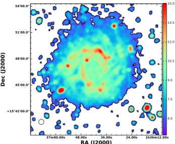
6.0 7.5 9.0 10.5 12.0 13.5 15.0Fig. 12: Strength of the total magnetic field at 1800resolution, in
units ofµG, determined by assuming energy equipartition.
Low-frequency observations will greatly help along with CRE modelling with time-dependent injection profiles. This is a topic of further investigation.
4.4. Magnetic field strength of NGC 628
The total magnetic field strength of NGC 628 can be determined from the nonthermal emission by assuming equipartition be-tween the energy densities of cosmic rays and magnetic field, using the revised formula of Beck & Krause (2005). The total magnetic field strength scales with the synchrotron intensity Isyn
as:
Btot,⊥ =Isyn/((K0+1)L)1/(3−αn) (4)
where Btot,⊥is the strength of the total field perpendicular to the
line of sight. Further assumptions required are the synchrotron spectral index ofαn=-1.0 and the effective path length through
the source ofL=1000 pc/cosi'1007 pc whereiis the inclina-tion of the galaxy. We also assumed that the polarised emission emerges from ordered fields in the galaxy plane. The adopted ratio of CR proton to electron number densities ofK0 =100 is
a reasonable assumption in the star-forming regions in the disk (Bell 1978). Realistic uncertainties in L and K0 of a factor of
about two would effect the result only by about 20%. The effect of adjustingαto between -0.7 and -0.9 produces an error of less than 5% in magnetic field strength. Using these assumptions, we created an image of the total magnetic field in NGC 628 from the nonthermal map (Fig. 10, right) which is shown in Fig. 12.
The mean total magnetic field strength is around 9µG and 11–12µG in the spiral arm regions (Fig. 12). The largest and brightest star-forming complexes seen across the spiral arms have a total magnetic field strength around 14µG, with a max-imum strength greater than 15µG in the star-forming complex in the north. In the extended disk of the galaxy (a galactic cen-tric radius of∼8.2 kpc) we observe a magnetic field strength of approximately 8µG.
NGC 628 has a similar magnetic field strength as NGC 6946 but a somewhat smaller field strength compared to IC 342 (Beck 2015), where the mean magnetic field strength is 14–15µG in the spiral arms. The main difference between NGC 628 and other galaxies in this respect is the central region, with a lower total
Fig. 13: Polarised emission following the largest HIIcomplexes
in the galaxy. Polarised intensity and magnetic vectors are over-laid onto an Hαimage (Dale et al. 2009). Contours of polarised intensity are at 9, 15, 24, and 30µJy/beam. The resolution of the JVLA image at 1000 is illustrated by the ellipse located in the bottom left corner.
magnetic field strength of 9-10µG compared to the central re-gions of NGC 6946 (about 25µG) (Beck 2007) and of IC 342 (about 30µG) (Beck 2015).
This method of calculating the total magnetic field strength most likely causes an underestimation of the magnetic field strength especially in the centre of the galaxy and extended disk due to the uncertainty ofK0 caused by ageing of CREs
propa-gating into regions of low star formation. Ideally, low-frequency observations would be far more useful in determining the mag-netic field strengths, not being contaminated by thermal emission (Mulcahy et al. 2014).
4.5. Polarised intensity
Images of linearly polarised intensity with overlaid B-vectors at 1000and 1800resolutions are shown in the lower panels of Figs. 5
and 6. These maps were obtained by averaging Q and U over all channels, without correction for the effects of Faraday rotation between the channels.
Ordered magnetic fields are traced by polarised synchrotron emission and form spiral patterns in nearly every galaxy (Beck 2016), even in flocculent (Soida et al. 2002) and ring galax-ies (Chy˙zy & Buta 2008). In NGC 628, three polarisation arms are prominent and are labeled in Fig 5. These arms resemble the arms observed in IC 342 (Krause 1993; Beck 2015) and NGC 6946 (Beck 2007).
The first and most prominent polarisation spiral arm (arm 1) runs counter-clockwise, starting along the large HIIregions in
the north-west, which are seen in total intensity (Fig. 4). This indicates that a fraction of the isotropic turbulent field is com-pressed or sheared and has become anisotropic turbulent. The region at the most northern point has the brightest polarised flux density and several interesting features makes it stand out from the rest of the galaxy. This region will be discussed in more de-tail in Sect. 5.5. Arm 1 spreads out into the inter-arm region of the galaxy in the south-east and continues to the south. The pitch
Fig. 14: Close-up of the magnetic arms located in an interarm re-gion shown with polarised intensity and magnetic vectors over-laid onto an optical DSS image. Contours of polarised intensity are at 10, 20µJy/beam. The resolution of the JVLA image at 1000 is illustrated by the ellipse located in the bottom left corner.
angle of the polarisation vectors decreases along arm 1, from about 50◦in the north-west to about 30◦in the east and south (see Table 8).
The spiral arm features in polarised intensity are located mostly between the optical arms, except in the inner (north-western and northern) parts of the polarisation arm 1 (at approx-imately RA(J2000)=01h36m37–41s; DEC(J2000)= +15◦470–
490). Here, the polarised emission closely follows the HII
com-plexes (Fig. 13). At small radii the polarised emission is located at the inner edge of the optical spiral arm and then crosses the ridge line delineated by HIIregions to the outer edge of the arm.
Finally, the polarisation coincides with a bright HIIcomplex.
The second and less prominent polarisation arm (arm 2) be-gins south-east of the centre of the galaxy and travels to the south-west. Arm 2 is narrower than arm 1. Another narrow arm (arm 3) begins in the south and continues into the extended disk in the north-west. The pitch angle of the polarisation vectors in arms 2 and 3 are large (about 45◦) and do not vary significantly with increasing distance from the galaxy’s centre (see Table 8). Arms 2 and 3 resemble magnetic arms4.
They are clearly offset from the optical arm (Figs. 5 and 14), narrow (about 1.1 kpc), and show a high degree of polarisation to the total intensity (on average 25% and up to 40% locally).
4 For polarised arms to be considered magnetic arms they must follow the required criteria as defined by Beck (2015):
– exist entirely in the interarm region of the galaxy, i.e between the optical arms
– be narrow (≈1 kpc) and filamentary with an almost constant pitch angle
– have a high degree of polarisation
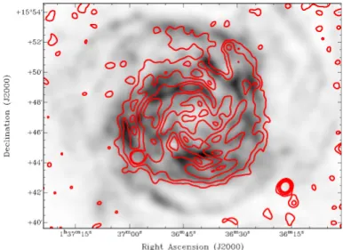
Fig. 15: Overlay of the polarised radio continuum emission onto the HITHINGS data, both smoothed to the same resolution of
3000. Contours are shown at 40, 80, 120µJy/beam.
Both polarisation spiral arms are partly coincident with the HIgas (THINGS data, Walter et al. (2008)), as shown in Fig. 15.
Given that the Faraday depolarisation at this frequency is small (Fig. 20) and the inclination is low, we do not expect to detect any more polarisation arms. The polarisation arms may extend even further into the outer disk, especially the polarisation (mag-netic) arm 3 in the north-west.
We find degrees of polarisation for the inner polarisation arms between 10–25% at small radii, increasing to 50 % at larger radii. This indicates an exceptionally ordered field. These de-grees of polarisation are comparable to those at 1.5 GHz mea-sured by Heald et al. (2009) while we are able to detect signifi-cantly more polarisation, especially in the northern region of the galaxy, due to the smaller amount of depolarisation at 3.1 GHz.
A number of background sources are seen in polarisation, those closest to the phase centre are shown in Table 7. These sources are used to estimate the Faraday depth for the Galactic foreground in Sect. 5.3.
4.6. Radial scale lengths of the radio continuum emission The observed extent of disk emission is sensitivity limited. To characterise the emission along the disk we use the exponential scale lengthl, that isIν∝exp(−r/l) whereris the galactocentric radius.
The radial profile of NGC 628 at 3.1 GHz was taken from the total, nonthermal, thermal and polarised intensities averaged in concentric rings with the position angle of the major axis and the inclination of the galaxy taken into account, using the val-ues from Table 1. Surrounding background point sources were removed by fitting and subtracting Gaussians before measuring the radial profile. Several background point sources located be-hind the inner disk were blanked out.
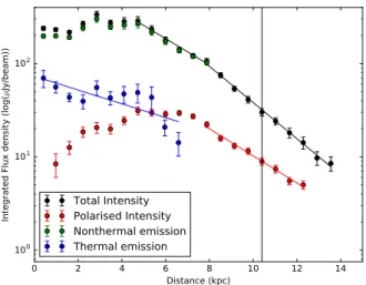
Fitting a single exponential profile is not possible, as a change in the slope of the total, nonthermal and polarised emis-sion occurs at several points in the radial profile (Fig. 16). One such break in the slope occurs at approximately 6.5 kpc which is approximately the radius where the star-formation rate declines. This is the location where thermal emission and the injection of fresh CREs ends. Such a change of slope was a result in the cos-mic ray electron propagation model of Mulcahy et al. (2016) for
0 2 4 6 8 10 12 14 Distance (kpc) 100 101 102 Int eg rat ed Fl ux de nsi ty (lo g( µ Jy/ be am )) Total Intensity Polarised Intensity Nonthermal emission Thermal emission
Fig. 16: Radial profile of NGC 628 for the total, nonthermal, thermal, and polarised radio intensities. The vertical line marks R25.
the galaxy M 51, using a realistic distribution of the injection of CREs. Beyond this radius, the total, nonthermal and polarised emission decrease exponentially.
It is unlikely that the lack of short spacings can cause the break in the radial profile of NGC 628. The largest angular scale of the JVLA at D configuration at S-band is 49000, comparable
to the angular size of NGC 628 (Table 1). To double check this, the JVLA map was smoothed and regridded to the same grid size as the Effelsberg 2.6 GHz map and subtracted. No signifi-cant residual flux density was observed meaning that the JVLA observation was able to detect the same structures as the single-dish observation, resulting in no missing flux density.
As there is a lack of emission at the centre of the galaxy in the total intensity, nonthermal, and polarised intensity maps, we were not able to fit an exponential function from the centre of the galaxy. Two separate exponential functions were fitted to the total intensity radial profile, inner (4–6 kpc) and outer disk (≥
6.5 kpc) for both images:
I(R)=
(
I4exp(−r/linner) 4 kpc≤r≤6.5 kpc
I6.5exp(−r/louter) r≥6.5 kpc. (5)
As linnercannot be fit to the polarised intensity radial profile,
only louterwas fitted. The thermal emission profile extracted from
HIIdisplays an overall exponential decrease,with an arm region
enhancement observed between 3 and 5 kpc. Here we fitted a single exponential function.
The radial profiles of the continuum emission for the total, nonthermal, thermal, and polarised intensity with the fitted func-tions are shown in Fig. 16. The obtained scale lengths for the inner and outer parts of the galaxy are given in Table 6.
Many galaxies studied possess a radial profile where the maximum flux density is observed at the centre of the galaxy and decreases exponentially usually displaying arm and inter-arm features. Such galaxies include M 33 (Tabatabaei et al. 2007b), M 51 (Mulcahy et al. 2014), IC 342 (Beck 2015), and M 101 (Berkhuijsen et al. 2016).
In contrast, NGC 628 is much more complicated, indicating that a continuous injection of CREs, especially in the central re-gion of the galaxy, is not valid. The total, nonthermal, and po-larised emission show a minimum in the centre of the galaxy,
Table 6: Scale lengths of the inner and outer disk of NGC 628.
linner(kpc) louter(kpc)
Total intensity 3.1±0.2 2.24±0.1
Polarised intensity - 3.0±0.1
Thermal intensity 5.8±1.2
-peaking at around 3-4 kpc, the polarised emission -peaking fur-thest out at 4 kpc. NGC 628 is unique with this absence of a bright central region and, as explained in Subsect. 4.3, the CRE population is not sufficient to produce significant synchrotron emission.
5. Observing the vertical magnetic field of NGC 628
RM Synthesis (Brentjens & de Bruyn 2005; Heald 2009) allows us to measure Faraday rotation and investigate vertical magnetic fields. The resulting Faraday map sheds light on phenomena such as Parker loops and HIholes which shall now be described.
5.1. RM Synthesis
When linearly polarised electromagnetic radiation passes through a magnetic-ionic medium, the plane of polarisation will rotate in a process known as Faraday rotation. When the po-larised emission from a background source passes through a medium that is non-emitting (this type of medium is called a Faraday screen) or if Faraday rotation within the emitting medium is small (a Faraday thin medium), then the plane of po-larisation will rotate by the following amount in radians:
∆χ=RMλ2 (6)
whereλis the wavelength of the polarised emission and RM is the rotation measure whose unit is rad m−2and is defined as the
slope of the polarisation angle versusλ2. For more general situa-tions and in situasitua-tions when regions with more than one rotation measure within the telescope beam are present, rotation measure is replaced with the quantity “Faraday depth”φ. Faraday depth is defined as:
φ=0.812
Z telescope
source
ne(l)Bk(l)dl. (7)
Here ne(l) is the thermal electron density in cm−3, Bkis magnetic
field strength along the line of sight inµG, anddl is the path length in parsecs.
RM Synthesis is a novel approach (Brentjens & de Bruyn 2005) to extract the distribution of Faraday depths (“Faraday spectrum”) of a source through polarimetric data whose eff ec-tiveness depends on theλ2coverage of the observation. With the
JVLA’s large bandwidth, RM Synthesis is an ideal tool to inves-tigate the nature of the vertical magnetic field of NGC 628.
The data were averaged in frequency channels in bins of 8, resulting in 64 channels with a bandwidth of 16 MHz each. The maximum Faraday depth for this channel width at 2.6 GHz is 1477 rad m−2, much larger than what is expected for NGC 628. With the coverage inλ2, the maximum theoretical Faraday
res-olution is 570 rad m−2, while the maximum observable scale in
the Faraday spectrum is 458 rad m−2. The resulting RM Spread Function (RMSF) of thisλ2coverage is shown in Fig. 17.
We created channel images with natural weighting at a res-olution of 1800, using the mosaic option of the CASA clean
Fig. 17: The RMSF of the remaining unflagged data channels (2.6–3.6 GHz). Note due to the continuous bandwidth, the side-lobes of the RMSF are relatively low. The first sidelobe is ap-proximately 20% whereas it was 78% for WSRT SINGS (Heald et al. 2009).
task rather than mosaicing all the fields manually after clean-ing. These images then had the primary beam correction applied. Each channel was visually inspected for RFI and one channel was deemed unusable. Therefore the final number of channel im-ages used for RM Synthesis was 63.
RM Synthesis and RM Clean (Heald et al. 2009) were both applied to the data using thepyrmsynthsoftware5. A search for
large Faraday depths in NGC 628 was performed over the range of -2×10⁵rad m−2to+2×10⁵rad m−2 with a coarseφsampling of 1000 rad m−2. No such polarised emission was detected at
very large Faraday depths. Hence, RM Synthesis was performed only in the range -3000 rad m−2 to+3000 rad m−2 with a
sam-pling of 25 rad m−2. The rms noise measured in the Stokes Q and U cubes is 3.6 and 4.2µJy/beam, respectively.
The maximum Faraday depth (φmax) in the Faraday spectrum
at each pixel of the map was measured by fitting a parabola us-ing the three maximum points at the observed peak in the Fara-day spectrum. Only polarised flux densities above a 6σ level of 21.6µJy/beam were used. The Milky Way contribution (see Sect. 5.3) of -34 rad m−2was subtracted from this Faraday depth. The corresponding Q and U values were found from the near-est pixel to that of the measured maximum Faraday depth and were used to find the intrinsic polarisation angle (corrected for Faraday rotation via RM Synthesis) by:
χ0= 1 2arctan U(φmax) Q(φmax) ! . (8)
The magnetic field orientation is obtained by rotating the po-larisation angle by 90◦.
The polarised intensity image was created using the AIPS task ‘COMB’ with the ‘POLC’ options which takes into account the bias polarised intensity caused by noise in Stokes Q and U. We used the average rms noise of the Q and U maps to correct for this bias (see Equation 1). The polarised intensity map is very similar to the channel averaged image (Fig. 6). This is due to the fact that Faraday rotation between the frequency channels at this
5 https://mrbell.github.io/pyrmsynth/
frequency is small. The only significant difference is the slightly more extended emission seen in the south east of the galaxy.
The errors in Faraday depth and intrinsic polarisation angle were determined by:
∆φ=φrms f 2S R (9) and ∆χ0= 1 rad 2S R (10)
whereφrms f is the FWHM of the RMSF and SR is the signal-to-noise ratio of the polarised intensity.
The maps of maximum Faraday depth and associated error are shown in Fig. 18.
RM Synthesis has been performed on NGC 628 previously at 18 and 22 cm wavelengths with the WSRT by Heald et al. (2009) with a Faraday depth resolution of 144 rad m−2, with the
domi-nant Faraday depth component centred on -30 rad m−2. While their Faraday resolution was superior compared to the present work, the sidelobe level was much higher due to the gap between the 18 and 22 cm bands. Additionally, this work has much bet-ter angular resolution and sensitivity and therefore we are able to resolve different features in our Faraday depth map (Fig. 18 left).
The main Faraday depth component observed in NGC 628 varies between+100 rad m−2and -110 rad m−2. The mean
Fara-day depth is -8 rad m−2with a standard deviation of 30 rad m−2. This agrees with the dominant Faraday depth component at -30 rad m−2 observed by Heald et al. (2009). The standard
devia-tion of 30 rad m−2contains real structure that is likely to be com-plex. The presence of a vertical magnetic field and the large scale height of cosmic-ray electrons tend to make the standard devi-ation of the Faraday dispersion function larger (Ideguchi et al. 2014).
We see an interesting and striking periodic pattern alternating between negative and positive Faraday depth values in the north-ern and eastnorth-ern parts of arm 1. In the southnorth-ern part of arm 1 no such pattern is seen, and the Faraday depths are mostly positive. Arms 2 and 3 neither show such a periodic pattern nor any ob-vious large-scale pattern in Faraday depth but has more negative Faraday depths than the southern part of arm 1 (see Sections 5.8 and 6.2 for details).
Braun et al. (2010) detected secondary components for NGC 628 at φ =-213 and +145 rad m−2 in addition to other
mildly inclined galaxies such as NGC 6946 and M 51. These secondary components may originate from polarisation at the far side of the midplane, becoming more Faraday rotated when pass-ing through the midplane, resultpass-ing in larger values of Faraday depths, approximately±200 rad m−2. Mao et al. (2015) searched
for these secondary components in M 51 with the JVLA at L-band and did not detect any significant polarisation coinciding with these secondary components. We have searched the Fara-day cube at 1800 and could not find indications in the Faraday spectra of these secondary components. It should be noted, how-ever, that the Faraday depth resolution for this observation is not enough to fully resolve the main component from the secondary components.
5.2. Magnetic field order
The nonthermal polarisation degree pn is a measure of the ra-tioq of the field strength of the ordered field in the sky plane
Fig. 18: Maps of the maximum fitted Faraday depthφmax(left) and the corresponding Faraday depth errorσφ(right) at a resolution
of 1800marked by an ellipse in the bottom left. Both quantities are measured in units of rad m−2. The polarised arms defined in Fig. 5
are shown here marked in red.
and the random field, named the degree of order of the field, q = Breg/Bran (Beck 2007). The maximum possible degree of
polarisation is given byp0=(3−3αn)/(5−3αn) whereαnis the
nonthermal spectral index taken here as -1.0.
In case of equipartition between the energy densities of mag-netic field and cosmic rays (Beck 2007):
pn p0 = q2 (q2+1 3) (11) q' (pn/p0) [2(1−(pn/p0))] !0.5 (12) Fig. 19 shows the nonthermal polarisation degree (left) and the degree of magnetic field order (right) for NGC 628 in the case of equipartition which was derived from the polarised in-tensity map found from RM Synthesis (Fig. 18, left) and the nonthermal map (Fig. 10, right). q is almost zero in the opti-cal spiral arms, meaning that depolarisation is enhanced in the spiral arms.qincreases toward the outer radii, specifically in the inter-arm regions where q reaches 0.8 where depolarisation is low. An isolated region with a maximumqof 0.56 exists in the northern part of polarisation arm 1 and coincides with the region of the most intense polarised emission, surrounded byqvalues of around 0.2. This region will be discussed in further detail in Sect. 5.5.
5.3. Estimate of the Galactic foreground in the direction of NGC 628
Based on three polarised sources detected in the NGC 628 field, Heald et al. (2009) estimated that the likely Galactic foreground Faraday depth is about -34±2 rad m−2. In our NGC 628 field we detect seven polarised sources, four of which are not directly located behind NGC 628. Table 7 shows the locations, Faraday depths, and polarised intensities of these discrete sources. The average of the Faraday depth of these four sources gives us a likely value of -20±14 rad m−2. It is possible that the Faraday depth of these sources used is still affected by NGC 628. These
sources are found in the range of 16–23 kpc from the centre of NGC 628. Han et al. (1998) found through RM data of back-ground sources that in M 31 the regular magnetic field probably extends to a radius of 25 kpc.
A Galactic foreground Faraday depth of -20±14 rad m−2 is
comparable to that of Heald et al. (2009). As the Faraday depth resolution in Heald et al. (2009) was superior to that of our work, -34 rad m−2was taken as the likely value when subtracting the Galactic foreground contamination. This also highlights the im-portance of L-band observations to achieve better Faraday depth resolution and thus ensure a more accurate removal of the Fara-day rotation caused by the Galactic foreground.
5.4. Depolarisation within S-Band
Faraday depolarisation is an important tool in retrieving infor-mation on the density of ionised gas, the strength of the ordered and turbulent field components, and the typical length scale (or integral scale) of turbulent magnetic fields. Significant depolar-isation is to be expected for NGC 628, as Heald et al. (2009) observed little to no polarised emission in the northern regions of the galaxy.
In order to get an estimation of the Faraday depolarisation we define the ratio DP (Beck 2007) by:
DP= PI2.87 GHz PI3.43 GHz ! × 3.43 GHz 2.87 GHz !αn (13)
whereαn=-1.0 is the nonthermal spectral index and is assumed
to be constant across the entire galaxy. DP=1 signifies no depo-larisation and DP=0 means total depolarisation. We image two sections of the band which have the same λ2 coverage. These
two bands have central frequencies of 2.87 & 3.43 GHz. The computed depolarisation map is shown in Fig. 20. We observe depolarisation ratios between 0.6 and 1.4 but the largest ratios are uncertain due to low signal-to-noise ratios. DP is about 0.9 on average and 0.7 in star-forming regions. Varyingαn by 0.2
changes the DP ratio by 0.03, likewise a 10% difference in po-larised intensity changes DP by 0.1.