Accelerating the DC algorithm for smooth functions

https://doi.org/10.1007/s10107-017-1180-1

F U L L L E N G T H PA P E R

Accelerating the DC algorithm for smooth functions

Phan T. Vuong2

Received: 27 July 2015 / Accepted: 8 July 2017 / Published online: 17 July 2017 © The Author(s) 2017. This article is an open access publication

Abstract We introduce two new algorithms to minimise smooth difference of convex (DC) functions that accelerate the convergence of the classical DC algorithm (DCA). We prove that the point computed by DCA can be used to define a descent direc-tion for the objective funcdirec-tion evaluated at this point. Our algorithms are based on a combination of DCA together with a line search step that uses this descent direc-tion. Convergence of the algorithms is proved and the rate of convergence is analysed under the Łojasiewicz property of the objective function. We apply our algorithms to a class of smooth DC programs arising in the study of biochemical reaction networks, where the objective function is real analytic and thus satisfies the Łojasiewicz prop-erty. Numerical tests on various biochemical models clearly show that our algorithms outperform DCA, being on average more than four times faster in both computational time and the number of iterations. Numerical experiments show that the algorithms are

F. J. Aragón Artacho was supported by MINECO of Spain and ERDF of EU, as part of the Ramón y Cajal program (RYC-2013-13327) and the Grant MTM2014-59179-C2-1-P. R. M. Fleming and P. T. Vuong were supported by the U.S. Department of Energy, Offices of Advanced Scientific Computing Research and the Biological and Environmental Research as part of the Scientific Discovery Through Advanced Computing program, Grant #DE-SC0010429.

B

[email protected]

1 _{Department of Mathematics, University of Alicante, Alicante, Spain} 2 _{Systems Biochemistry Group, Luxembourg Centre for Systems Biomedicine,}

globally convergent to a non-equilibrium steady state of various biochemical networks, with only chemically consistent restrictions on the network topology.

Keywords DC function·DC programming·DC algorithm·Łojasiewicz property· Biochemical reaction networks

Mathematics Subject Classification 65K05·65K10·90C26·92C42

1 Introduction

Many problems arising in science and engineering applications require the develop-ment of algorithms to minimise a nonconvex function. If a nonconvex function admits a decomposition, this may be exploited to tailor specialised optimisation algorithms. Our main focus is the following optimisation problem

minimise

x∈Rm φ(x):= f1(x)− f2(x), (1)

where f1,f2:Rm →Rare continuously differentiable convex functions and inf

x∈Rmφ(x) >−∞. (2)

In our case, as we shall see in Sect.4, this problem arises in the study of biochemical reaction networks. In general,φis a nonconvex function. The function in problem (1) belongs to two important classes of functions: the class of functions that can be decom-posed as a sum of a convex function and a differentiable function (composite functions) and the class of functions that are representable as difference of convex functions (DC functions).

In 1981, Fukushima and Mine [7,17] introduced two algorithms to minimise a

composite function. In both algorithms, the main idea is to linearly approximate the differentiable part of the composite function at the current point and then minimise the resulting convex function to find a new point. The difference between the new and current points provides a descent direction with respect to the composite function, when it is evaluated at the current point. The next iteration is then obtained through a line search procedure along this descent direction. Algorithms for minimising com-posite functions have been extensively investigated and found applications to many problems such as: inverse covariance estimate, logistic regression, sparse least squares and feasibility problems, see e.g. [9,14,15,19] and the references quoted therein.

In 1986, Pham Dinh and El Bernoussi [23] introduced an algorithm to minimiseDC functions. In its simplified form, theDifference of Convex functions Algorithm(DCA) linearly approximates the concave part of the objective function (−f2in (1)) at the cur-rent point and then minimises the resulting convex approximation to the DC function to find the next iteration, without recourse to a line search. The main idea is similar to Fukushima–Mine approach but was extended to the non-differentiable case. This algorithm has been extensively studied by Le Thi, Pham Dinh and their collaborators, see e.g. [10,12,13,22]. DCA has been successfully applied in many fields, such as

machine learning, financial optimisation, supply chain management and telecommu-nication [6,10,24]. Nowadays, DC programming plays an important role in nonconvex programming and DCA is commonly used because of its key advantages: simplicity, inexpensiveness and efficiency [10]. Some results related to the convergence rate for special classes of DC programs have been also established [11,13].

In this paper we introduce two new algorithms to find stationary points of DC programs, calledBoosted Difference of Convex function Algorithms(BDCA), which accelerate DCA with a line search using an Armijo type rule. The first algorithm directly uses a backtracking technique, while the second uses a quadratic interpolation of the objective function together with backtracking. Our algorithms are based on both DCA and the proximal point algorithm approach of Fukushima–Mine. First, we compute the point generated by DCA. Then, we use this point to define the search direction. This search direction coincides with the one employed by Fukushima–Mine in [7]. The key difference between their method and ours is the starting point used for the line search: in our algorithms we use the point generated by DCA, instead of using the previous iteration. This scheme works thanks to the fact that the defined search direction is not only a descent direction for the objective function at the previous iteration, as observed by Fukushima–Mine, but is also a descent direction at the point generated by DCA. Unfortunately, as shown in Remark 1, this scheme cannot be extended in general for nonsmooth functions, as the defined search direction might be an ascent direction at the point generated by DCA.

Moreover, it is important to notice that the iterations of Fukushima–Mine and BDCA never coincide, as the largest step size taken in their algorithm is equal to one (which gives the DCA iteration). In fact, for smooth functions, the iterations of Fukushima– Mine usually coincide with the ones generated by DCA, as the step size equal to one is normally accepted by their Armijo rule.

We should point out that DCA is a descent method without line search. This is something that is usually claimed to be advantageous in the large-scale setting. Our purpose here is the opposite: we show that a line search can increase the performance even for high-dimensional problems.

Further, we analyse the rate of convergence under the Łojasiewicz property [16] of the objective function. It should be mentioned that the Łojasiewicz property is recently playing an important role for proving the convergence of optimisation algorithms for analytic cost functions, see e.g. [1,3,4,13].

We have performed numerical experiments in functions arising in the study of biochemical reaction networks. We show that the problem of finding a steady state of these networks, which plays a crucial role in the modelling of biochemical reaction systems, can be reformulated as a minimisation problem involving DC functions. In fact, this is the main motivation and starting point of our work: when one applies DCA to find a steady state of these systems, the rate of convergence is usually quite slow. As these problems commonly involve hundreds of variables (even thousands in the most complex systems, as Recon 21), the speed of convergence becomes crucial. In 1 _{Recon 2 is the most comprehensive representation of human metabolism that is applicable to}

computa-tional modelling [25]. This biochemical network model involves more than four thousand molecular species and seven thousand reversible elementary reactions.

our numerical tests we have compared BDCA and DCA for finding a steady state in various biochemical network models of different size. On average, DCA needed five times more iterations than BDCA to achieve the same accuracy, and what is more relevant, our implementation of BDCA was more than four times faster than DCA to achieve the same accuracy. Thus, we prove both theoretically and numerically that BDCA results more advantageous than DCA. Luckily, the objective function arising in these biochemical reaction networks is real analytic, a class of functions which is known to satisfy the Łojasiewicz property [16]. Therefore, the above mentioned convergence analysis results can be applied in this setting.

The rest of this paper is organised as follows. In Sect.2, we recall some prelimi-nary facts used throughout the paper and we present the main optimisation problem. Sect.3describes our main results, where the new algorithms (BDCA) and their con-vergence analysis for solving DC programs are established. A DC program arising in biochemical reaction network problems is introduced in Sect.4. Numerical results comparing BDCA and DCA on various biochemical network models are reported in Sect.5. Finally, conclusions are stated in the last section.

2 Preliminaries

Throughout this paper, the inner product of two vectorsx,y∈Rmis denoted byx,y, while · denotes the induced norm, defined byx = √x,x. The nonnegative orthant inRm is denoted byRm₊ = [0,∞)m andB(x,r)denotes the closed ball of centerxand radiusr >0. The gradient of a differentiable function f :Rm →Rnat some pointx∈Rmis denoted by∇f(x)∈Rm×n.

Recall that a function f :Rm →Ris said to beconvexif

f(λx+(1−λ)y)≤λf(x)+(1−λ)f(y) for allx,y∈Rmandλ∈(0,1). Further, f is calledstrongly convexwith modulusσ >0 if

f (λx+(1−λ)y)≤λf(x)+(1−λ)f(y) −1

2σλ(1−λ)x−y

2 _{for allx,y∈R}m_{andλ∈(0,1),}

or, equivalently, when f −σ₂ · 2is convex. The function f is said to becoerciveif

f(x)→ +∞wheneverx → +∞.

On the other hand, a functionF :Rm →Rmis said to bemonotonewhen

F(x)−F(y),x−y ≥0 for allx,y∈Rm.

Further,Fis calledstrongly monotonewith modulusσ >0 when

F(x)−F(y),x−y ≥σx−y2 for allx,y∈Rm.

The functionF is calledLipschitz continuousif there is some constant L ≥ 0 such that

Fis called locally Lipschitz continuous if for everyxinRm, there exists a neighbour-hoodU ofxsuch thatF restricted toUis Lipschitz continuous.

We have the following well-known result.

Proposition 1 Let f : Rm → Rbe a differentiable function. Then f is (strongly) convex if and only if∇f is (strongly) monotone.

To establish our convergence results, we will make use of the Łojasiewicz property, defined next.

Definition 1 Let f :Rn_{→Rbe a differentiable function.}

(i) The function f is said to have the Łojasiewicz propertyif for any critical pointx¯, there exist constantsM >0, ε >0 andθ∈ [0,1)such that

|f(x)− f(x¯)|θ≤M∇f(x), for allx∈B(x¯, ε), (3) where we adopt the convention 00 = 0. The constantθ is called Łojasiewicz exponentof f atx¯.

(ii) The function f is said to bereal analyticif for everyx∈Rn_{,f may be represented}

by a convergent power series in some neighbourhood ofx.

Proposition 2 [16]Every real analytic function f :Rn→Rsatisfies the Łojasiewicz property with exponentθ∈[0,1).

Problem (1) can be easily transformed into an equivalent problem involving strongly convex functions. Indeed, choose any ρ > 0 and consider the functions g(x) :=

f1(x)+ ρ₂x2 _{and h(x) := f2(x)+} ρ

2x2. Then g andh are strongly convex

functions with modulusρandg(x)−h(x)=φ(x), for allx ∈Rm_{. In this way, we}

obtain the equivalent problem

(P) minimise

x∈Rm φ(x)=g(x)−h(x). (4)

The key step to solve(P)with DCA is to approximate the concave part−hof the objective functionφby its affine majorisation and then minimise the resulting convex function. The algorithm proceeds as follows.

ALGORITHM 1:(DCA, [12])

1. Letx0be any initial point and setk:=0.

2. Solve the strongly convex optimisation problem

(Pk) minimise

x∈Rm g(x)− ∇h(xk),x.

to obtain the unique solutionyk.

3. Ifyk=xkthen STOP and RETURNxk, otherwise setxk+1:=yk, setk:=k+1, and go to

In [7] Fukushima and Mine adapted their original algorithm reported in [17] by adding a proximal term ρ₂x−xk2to the objective of the convex optimisation

sub-problem. As a result they obtain an optimisation subproblem that is identical to the one in Step 2 of DCA, when one transforms (1) into (4) by adding ρ₂x2_{to each}

convex function. In contrast to DCA, Fukushima–Mine algorithm [7] also includes a line search along the directiondk :=yk−xkto find the smallest nonnegative integer lksuch that the Armijo type rule

φxk+βlkdk

≤φ(xk)−αβlkdk2 (5)

is satisfied, whereα >0 and 0< β <1. Thus, whenlk=0 satisfies (5), i.e. when

φ(yk)≤φ(xk)−αdk2,

one hasxk+1=yk and the iterations of both algorithms coincide. As we shall see in

Proposition3, this is guaranteed to happen ifα≤ρ.

3 Boosted DC Algorithms

Let us introduce our first algorithm to solve(P), which we call aBoosted DC Algo-rithm with Backtracking. The algorithm is a combination of Algorithm 1 and the algorithm of Fukushima–Mine [7].

ALGORITHM 2:(BDCA-Backtracking)

1. Fixα >0,λ >¯ 0 and 0< β <1. Letx0be any initial point and setk:=0.

2. Solve the strongly convex minimisation problem

(Pk)minimise

x∈Rm g(x)− ∇h(xk),x

to obtain the unique solutionyk.

3. Setdk:=yk−xk. Ifdk=0, STOP and RETURNxk. Otherwise, go to Step 4.

4. Setλk:= ¯λ. WHILEφ(yk+λkdk) > φ(yk)−αλkdk2DOλk:=βλk.

5. Setxk+1:=yk+λkdk. Ifxk+1=xkthen STOP and RETURNxk, otherwise setk:=k+1,

and go to Step 2.

The next proposition shows that the solution of(Pk), which coincides with the

DCA subproblem in Algorithm 1, provides a decrease in the value of the objective function. For the sake of completeness, we include its short proof.

Proposition 3 For all k∈N, it holds that

φ(yk)≤φ(xk)−ρdk2. (6)

Proof Sinceykis the unique solution of the strongly convex problem(Pk), we have ∇g(yk)= ∇h(xk), (7)

which implies

g(xk)−g(yk)≥ ∇h(xk),xk−yk + ρ

2xk−yk

2_.

On the other hand, the strong convexity ofhimplies

h(yk)−h(xk)≥ ∇h(xk),yk−xk + ρ

2yk−xk

2_.

Adding the two previous inequalities, we have

g(xk)−g(yk)+h(yk)−h(xk)≥ρxk−yk2,

which implies (6).

Ifλk =0, the iterations of BDCA-Backtracking coincide with those of DCA, since

the latter setsxk+1:=yk. Next we show thatdk =yk−xkis a descent direction for

φatyk. Thus, one can achieve a larger decrease in the value ofφby moving along

this direction. This simple fact, which permits an improvement in the performance of DCA, constitutes the key idea of our algorithms.

Proposition 4 For all k∈N, we have

∇φ(yk),dk ≤ −ρ||dk||2; (8) that is, dkis a descent direction forφat yk.

Proof The function h is strongly convex with constantρ. This implies that ∇h is strongly monotone with constantρ; whence,

∇h(xk)− ∇h(yk),xk−yk ≥ρxk−yk2.

Further, sinceykis the unique solution of the strongly convex problem(Pk), we have ∇h(xk)= ∇g(yk),

which implies,

∇φ(yk),dk = ∇g(yk)− ∇h(yk),dk ≤ −ρdk2,

and completes the proof.

Remark 1 In general, Proposition4does not remain valid whengis not differentiable. In fact, the directiondkmight be an ascent direction, in which case Step 4 in Algorithm 2

could become an infinite loop. For instance, consider g(x)= |x| + 1₂x2+ 1₂x and

h(x)= 1₂x2forx ∈R. Ifx0= 1₂, one has (P0)minimise x∈R |x| + 1 2x 2₊1 2x− 1 2x,

whose unique solution isy0=0. Then, the one-sided directional derivative ofφaty0

in the directiond0=y0−x0= −1₂is given by φ(y0;d0)=lim t↓0 φ (0+t(−1/2))−φ(0) t = 1 4.

Thus,d0is an ascent direction forφaty0(actually,y0is the global minimum ofφ). As a corollary, we deduce that the backtracking Step 4 of Algorithm 2 terminates finitely whenρ > α.

Corollary 1 Suppose thatρ > α. Then, for all k∈N,there is someδk>0such that

φ (yk+λdk)≤φ(yk)−αλdk2, for allλ∈ [0, δk]. (9) Proof Ifdk = 0 there is nothing to prove. Otherwise, by the mean value theorem,

there is somet_λ∈(0,1)such that

φ (yk+λdk)−φ(yk)= ∇φ (yk+tλλdk) , λdk

=λ∇φ(yk),dk +λ∇φ(yk+t_λλdk)− ∇φ(yk),dk ≤ −ρλdk2+λ∇φ (yk+t_λλdk)− ∇φ(yk)dk.

As∇φis continuous atyk, there is someδ >0 such that

∇φ(z)− ∇φ(yk) ≤(ρ−α)dkwheneverz−yk ≤δ.

Sinceyk+tλλdk−yk =tλλdk ≤λdk, then for allλ∈

0,_dδ k , we deduce φ(yk+λdk)−φ(yk)≤ −ρλdk2+(ρ−α)λdk2= −αλdk2,

and the proof is complete.

Remark 2 Notice that yk+λdk =xk+(1+λ)dk. Therefore, Algorithm 2 uses the

same direction as the Fukushima–Mine algorithm [7], wherexk₊1 = xk +βldk =

βl_y k+

1−βlxkfor some 0< β <1 and some nonnegative integerl. The iterations

would be the same ifβl _{=λ+1. Nevertheless, as 0< β <1, the step sizeλ=β}l₋₁

chosen in the Fukushima–Mine algorithm [7] is always less than or equal to zero, while in Algorithm 2, only step sizes λ ∈ ]0,λ¯]are explored. Moreover, observe that the Armijo type rule (5), as used in [7], searches for anlksuch thatφ(xk+βlkdk) < φ(xk),

whereas Algorithm 2 searches for aλk such that φ(yk+λkdk) < φ(yk). We know

from (6) and (9) that

φ (yk+λdk)≤φ(yk)−αλdk2≤φ(xk)−(ρ+αλ)dk2;

thus, Algorithm 2 results in a larger decrease in the value ofφat each iteration than DCA, which setsλ:=0 andxk₊1:=yk. Therefore, a faster convergence of Algorithm

Remark 3 In a personal communication, Christian Kanzow pointed out that the assumption ρ > α can be removed if one replaces the step size rule (9) by φ (yk+λdk) ≤ φ(yk)−αλ2dk2.It can be easily checked that the convergence

theory in the rest of the paper remains valid with some small adjustments.

The following convergence results were inspired by Attouch and Bolte [3], which in turn were adapted from the original ideas of Łojasiewicz; see also [5, Section 3.2].

Proposition 5 For any x0∈Rm, either Algorithm 2 returns a stationary point of(P) or it generates an infinite sequence such that the following holds.

(i) φ(xk)is monotonically decreasing and convergent to someφ∗.

(ii) Any limit point of{xk}is a stationary point of(P). If in addition,φis coercive then there exits a subsequence of {xk}which converges to a stationary point of(P).

(iii) ∞k₌0dk2<∞and∞k₌0xk₊1−xk2<∞.

Proof Because of (7), if Algorithm 2 stops at Step 3 and returnsxk, thenxkmust be

a stationary point of(P). Otherwise, by Proposition3and Step 4 of Algorithm 2, we have

φ(xk₊1)≤φ(yk)−αλkdk2≤φ(xk)−(αλk+ρ)dk2. (10)

Hence, as the sequence{φ(xk)}is monotonically decreasing and bounded from below

by (2), it converges to someφ∗, which proves (i). Consequently, we have φ(xk+1)−φ(xk)→0.

Thus, by (10), one hasdk2= yk−xk2→0.

Letx¯be any limit point of{xk}, and let{xki}be a subsequence of{xk}converging

tox¯. Sinceyki −xki →0, one has

yki → ¯x.

Taking the limit asi → ∞in (7), as∇h and∇g are continuous, we have∇h(x¯)= ∇g(x¯).

Ifφis coercive, since the sequence{φ(xk)}is convergent, then the sequence{xk}

is bounded. This implies that there exits a subsequence of{xk}converging tox¯, a

stationary point of(P), which proves (ii). To prove (iii), observe that (10) implies that

(αλk+ρ)dk2≤φ(xk)−φ(xk+1). (11)

Summing this inequality from 0 toN, we obtain

N

k=0

(αλk+ρ)dk2≤φ(x0)−φ(xN+1)≤φ(x0)− inf

whence, taking the limit whenN → ∞, ∞ k=0 ρdk2≤ ∞ k=0 (αλk+ρ)dk2≤φ(x0)− inf x∈Rmφ(x) <∞, so we have∞_k=0dk2<∞. Since xk+1−xk=yk−xk+λkdk=(1+λk)dk, we obtain ∞ k=0 xk₊1−xk2= ∞ k=0 (1+λk)2dk2≤(1+ ¯λ)2 ∞ k=0 dk2<∞,

and the proof is complete.

We will employ the following useful lemma to obtain bounds on the rate of convergence of the sequences generated by Algorithm 2. This result appears within the proof of [3, Theorem 2] for specific values ofαandβ. See also [13, Theorem 3.3], or very recently, [15, Theorem 3].

Lemma 1 Let{sk}be a sequence in R+ and let α, β be some positive constants. Suppose that sk →0and that the sequence satisfies

sα_k ≤β(sk−sk+1), for all k sufficiently large. (13) Then

(i) ifα=0, the sequence{sk}converges to0in a finite number of steps;

(ii) ifα∈(0,1], the sequence{sk}converges linearly to0with rate1−_β1;

(iii) ifα >1, there existsη >0such that sk ≤ηk−

1

α−1, _{for all k sufficiently large.}

Proof Ifα=0, then (13) implies

0≤sk+1≤sk−

1 β, and (i) follows.

Assume thatα∈(0,1]. Sincesk →0, we have thatsk <1 for allklarge enough.

Thus, by (13), we have sk ≤skα ≤β(sk−sk+1). Therefore,sk+1≤ 1−1_β

Suppose now thatα > 1. If sk = 0 for some k, then (13) impliessk₊1 = 0.

Then the sequence converges to zero in a finite number of steps, and thus (iii) trivially holds. Hence, we will assume thatsk>0 and that (13) holds for allk≥N, for some

positive integerN. Consider the decreasing functionϕ : (0,+∞)→ Rdefined by ϕ(s):=s−α. By (13), fork≥ N, we have 1 β ≤(sk−sk+1) ϕ(sk)≤ sk sk+1 ϕ(t)dt=s 1−α k+1 −s 1−α k α−1 .

Asα−1>0, this implies that

s_k1−₊₁α−s_k1−α≥ α−1

β ,

for allk≥N. Thus, summing forkfromN toj−1≥N, we have

s1_j−α−s1_N−α ≥ α−1

β (j−N), which gives, for all j ≥N+1,

sj ≤ sN1−α+ α−1 β (j−N) 1 1−α . Therefore, there is someη >0 such that

sj ≤ηj−

1

α−1, _{for allksufficiently large,}

which completes the proof.

Theorem 1 Suppose that ∇g is locally Lipschitz continuous and φ satisfies the Łojasiewicz property with exponent θ ∈ [0,1). For any x0 ∈ Rm, consider the sequence{xk}generated by Algorithm 2. If the sequence{xk}has a cluster point x∗, then the whole sequence converges to x∗,which is a stationary point of(P). Moreover, denotingφ∗:=φ(x∗), the following estimations hold:

(i) ifθ=0then the sequences{xk}and{φ(xk)}converge in a finite number of steps to x∗andφ∗, respectively;

(ii) ifθ ∈ 0,1₂then the sequences{xk}and{φ(xk)}converge linearly to x∗ and

φ∗_{, respectively;}

(iii) ifθ∈1₂,1then there exist some positive constantsη1andη2such that xk−x∗ ≤η1k− 1−θ 2θ−1, φ(xk)−φ∗≤η2k− 1 2θ−1,

Proof By Proposition5, we have limk_→∞φ(xk)=φ∗. Ifx∗is a cluster point of{xk},

then there exists a subsequence{xki}of{xk}that converges tox∗. By continuity ofφ,

we have that

φ(x∗)= lim

i→∞φ(xki)=klim→∞φ(xk)=φ

∗_.

Hence,φis finite and has the same valueφ∗at every cluster point of{xk}. Ifφ(xk)=φ∗

for somek>1, thenφ(xk)=φ(xk+p)for any p ≥0, since the sequenceφ(xk)is

decreasing. Therefore,xk =xk+p for all p ≥ 0 and Algorithm 2 terminates after a

finite number of steps. From now on, we assume thatφ(xk) > φ∗for allk.

Asφsatisfies the Łojasiewicz property, there existM >0, ε1>0 andθ ∈ [0,1)

such that

|φ(x)−φ(x∗)|θ≤M∇φ(x), ∀x∈B(x∗, ε1). (14)

Further, as∇g is locally Lipschitz aroundx∗, there are some constants L ≥ 0 and ε2>0 such that

∇g(x)− ∇g(y) ≤Lx−y, ∀x,y∈B(x∗, ε2). (15)

Letε := 1₂min{ε1, ε2}>0. Since limi→∞xki =x∗and limi→∞φ(xki)=φ∗, we

can find an indexN large enough such that

xN−x∗ + M L1+ ¯λ (1−θ)ρ φ(xN)−φ∗ 1_−θ < ε. (16)

By Proposition5(iii), we know thatdk = yk−xk → 0. Then, taking a larger N if

needed, we can assure that

yk−xk ≤ε, ∀k≥N.

We now prove that, for allk≥ N, wheneverxk∈B(x∗, ε)it holds xk+1−xk ≤ M L(1+λk) (1−θ)(αλk+ρ) φ(xk)−φ∗ 1−θ −φ(xk+1)−φ∗ 1−θ (17)

Indeed, consider the concave functionγ :(0,+∞)→ (0,+∞)defined asγ (t):= t1−θ. Then, we have

γ (t1)−γ (t2)≥ ∇γ (t1)T(t1−t2), ∀t1,t2_>0.

Substituting in this inequality t1 by (φ(xk)−φ∗) and t2 by (φ(xk₊1)−φ∗) and

φ(xk)−φ∗ 1−θ −φ(xk+1)−φ∗ 1−θ ≥ 1−θ (φ(xk)−φ∗)θ (φ(xk)−φ(xk+1)) ≥ 1−θ M∇φ(xk)(αλ k+ρ)yk−xk2 = (1−θ) (αλk+ρ) M(1+λk)2∇φ(xk) xk+1−xk2. (18) On the other hand, since∇g(yk)= ∇h(xk)and

yk−x∗ ≤ yk−xk + xk−x∗ ≤2ε≤ε2, using (15), we obtain ∇φ(xk) = ∇g(xk)− ∇h(xk) = ∇g(xk)− ∇g(yk) ≤Lxk−yk = L (1+λk)x k+1−xk. (19)

Combining (18) and (19), we obtain (17). From (17), asλk ∈(0,λ¯], we deduce xk₊1−xk ≤ M L1+ ¯λ (1−θ)ρ φ(xk)−φ∗ 1−θ −φ(xk₊1)−φ∗ 1−θ , (20)

for allk≥N such thatxk ∈B(x∗, ε).

We prove by induction thatxk∈B(x∗, ε)for allk≥ N. Indeed, from (16) the claim

holds fork = N. We suppose that it also holds fork =N,N +1, . . . ,N +p−1, withp≥1. Then (20) is valid fork=N,N+1, . . . ,N+p−1. Therefore

xN+p−x∗≤xN−x∗+ p i₌1 xN+i−xN+i−1 ≤xN−x∗ + M L 1+ ¯λ (1−θ)ρ p i=1 φ(xN+i−1)−φ∗ 1−θ −φ(xN+i)−φ∗ 1−θ ≤xN−x∗+ M L1+ ¯λ (1−θ)ρ φ(xN)−φ∗ 1−θ < ε, where the last inequality follows from (16).

Adding (20) fromk=NtoPone has

P k=N xk+1−xk ≤ M L1+ ¯λ (1−θ)ρ φ(xN)−φ∗ 1−θ . (21)

Taking the limit asP → ∞, we can conclude that ∞

k=1

xk+1−xk<∞. (22)

This means that {xk}is a Cauchy sequence. Therefore, since x∗ is a cluster point

of {xk}, the whole sequence{xk}converges to x∗. By Proposition5,x∗ must be a

stationary point of(P).

Fork≥ N, it follows from (14), (15) and (11) that (φ(xk)−φ∗)2θ ≤M2∇φ(xk)2 ≤M2∇g(xk)− ∇h(xk)2=M2∇g(xk)− ∇g(yk)2 ≤M2L2xk−yk2≤ M2L2 αλk+ρ φ(xk)−φ(xk+1) ≤δφ(xk)−φ∗ −φ(xk+1)−φ∗ , (23)

where δ := M2_ρL2 > 0. By applying Lemma1 withsk := φ(xk)−φ∗,α := 2θ

andβ :=δ, statements (i)–(iii) regarding the sequence{φ(xk)}easily follow from (23).

We know thatsi :=

_∞

k=ixk+1−xkis finite by (22). Notice thatxi−x∗ ≤si

by the triangle inequality. Therefore, the rate of convergence ofxitox∗can be deduced

from the convergence rate ofsi to 0. Adding (20) fromi toPwithN ≤i ≤ P, we

have si = lim P→∞ P k₌i xk+1−xk ≤K1 φ(xi)−φ∗ 1−θ , whereK1:= M L₍₁₋(1_θ)ρ+¯λ)>0. Then by (14) and (15), we get

s θ 1−θ i ≤ M K θ 1−θ 1 ∇φ(xi) ≤M L K θ 1−θ 1 xi−yi ≤ M L K θ 1−θ 1 1+λi xi+1− xi ≤M L K θ 1−θ 1 xi+1−xi =M L K θ 1−θ 1 (si−si+1) Hence, takingK2:=M L K1−θθ

1 >0, for alli ≥ Nwe have s

θ 1−θ

i ≤ K2(si−si+1) .

By applying Lemma 1 withα := ₁₋θ_θ andβ := K2, we see that the statements

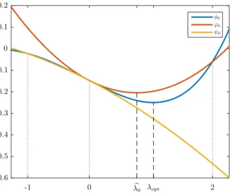
-1 -0.5 0 0.5 1 1.5 2 -0.25 -0.2 -0.15 -0.1 -0.05 0 Fig. 1 Plot ofφ 3 5(1+λ)− 27 125λ

forφ(x)= 1₄x4−1₂x2. As shown in Proposition4, the function is decreasing at 0. The valueλ = 0 corresponds to the next iteration chosen by DCA, while the next iteration chosen by algorithm [7] setsλ∈ ] −1,0]. Algorithm 2 chooses the next iteration takingλ∈ ]0,λ¯], which permits to achieve an additional decrease in the value ofφ. Here, the optimal value is attained atλopt=25₂₄≈1.04.

Example 1 Consider the functionφ(x)= 1₄x4− 1₂x2. The iteration given by DCA (Algorithm 1) satisfies

xk3+1−xk =0;

that is,xk+1=√3 xk. On the other hand, the iteration defined by Algorithm 2 is

xk+1=(1+λk)3

xk−λkxk.

If x0 = x0 = ₁₂₅27, we have x1 = 3₅, while x1 = 3₅(1+λ0)− ₁₂₅27λ0. For any

λ0 ∈ 0,25 √ 41−75 48

, we have φ(x1) < φ(x1). The optimal step size is attained at λopt= 25₂₄ withx1=1, which is the global minimiser ofφ.

Observe in Fig.1that the function

φk(λ):=φ (yk+λdk)

behaves as a quadratic function nearby 0. Then, a quadratic interpolation of this func-tion should give us a good candidate for choosing a step size close to the optimal one. Whenever ∇φ is not too expensiveto compute, it makes sense to construct a quadratic approximation ofφwith an interpolation using three pieces of information: φk(0)=φ(yk),φ_k(0)= ∇φ(yk)Tdkandφk(λ)¯ . This gives us the quadratic function

ϕk(λ):= φk(λ)¯ −φk(0)− ¯λφ_k(0) ¯ λ2 λ2_+φ k(0)λ+φk(0), (24)

see e.g. [20, Section 3.5]. Whenφk(λ) > φ¯ k(0)+ ¯λφ_k(0), the functionϕkhas a global

minimiser at λk := − φ k(0)λ¯2 2φk(λ)¯ −φk(0)−φ_k(0)λ¯ . (25)

This suggests the following modification of Algorithm 2.

Corollary 2 The statements inTheorem1also apply toAlgorithm3.

ALGORITHM 3:(BDCA-Quadratic Interpolation with Backtracking)

1. Fixα >0,λmax>λ >¯ 0 and 0< β <1. Letx0be any initial point and setk:=0.

2. Solve the strongly convex minimisation problem

(Pk)minimise

x∈Rm g(x)− ∇h(xk),x

to obtain the unique solutionyk.

3. Setdk:=yk−xk. Ifdk=0 STOP and RETURNxk. Otherwise, go to Step 4.

4. Computeλkas in (25). Ifλk>0 andφ(yk+λkdk) < φ(yk+ ¯λdk)setλk:=min λk, λmax;

otherwise, setλk:= ¯λ.

WHILEφ(yk+λkdk) > φ(yk)−αλkdk2DOλk:=βλk.

5. Setxk+1:=yk+λkdk. Ifxk+1=xkthen STOP and RETURNxk, otherwise setk:=k+1,

and go to Step 2.

Proof Just observe that the proof of Theorem1remains valid as long as the step sizes are bounded above by some constant and below by zero. Algorithm 3 uses the same directions than Algorithm 2, and the step sizes chosen by Algorithm 3 are bounded

above byλmaxand below by zero.

Another option here would be to construct a quadratic approximation ψk using

φk(−1)=φ(xk)instead ofφk(λ)¯ . This interpolation is computationally less

expen-sive, as it does not require the computation ofφk(λ)¯ . Nevertheless, our numerical tests

for the functions in Sect.4show that this approximation usually fits the functionφk

more poorly. In particular, this situation occurs in Example1, as shown in Fig.2. One could also construct a cubic function that interpolatesφk(−1),φk(0),φ_k(0)and

φk(λ)¯ , see [20, Section 3.5]. However, for the functions in Sect.4, we have observed

that this cubic function usually fits the functionφk worse than the quadratic function

ϕkin (24).

Remark 4 Observe that Algorithm 2 and Algorithm 3 still work well if we replace Step 2 by the following proximal step as in [18]

Fig. 2 Plots of the quadratic interpolationsϕ0andψ0for the functionφ0(λ) = φ(y0+λd0)from

Example1, withλ¯=2. Note thatψ0(λ)fits poorlyφ0(λ)forλ >0 (Pk) minimise

x∈Rm g(x)− ∇h(xk),x +

1 2ckx−

xk2,

for some positive constantsck.

Example 2 (Finding zeroes of systems of DC functions)

Suppose that one wants for find a zero of a system of equations

p(x)=c(x), x∈Rm (26) where p : Rm → Rm₊ and c : Rm → Rm₊ are twice continuously differentiable functions such that pi :Rm →R+andci :Rm →R+are convex functions for all i =1, . . . ,m. Then, p(x)−c(x)2=2 p(x)2+ c(x)2 − p(x)+c(x)2.

Observe that all the components of p(x)andc(x)are nonnegative convex functions. Hence, both f1(x) := 2p(x)2+ c(x)2 and f2(x) := p(x)+c(x)2 are continuously differentiable convex functions, because they can be expressed as a finite combination of sums and products of nonnegative convex functions. Thus, we can either apply DCA or BDCA in order to find a solution to (26) by settingφ(x) :=

f1(x)− f2(x).

Let f(x) := p(x)−c(x)forx ∈ Rm. Suppose that x¯ is an accumulation point of the sequence{xk}generated by either Algorithm 2 or Algorithm 3, and assume

that∇f(x¯)is nonsingular. Then, by Proposition5, we must have∇f(x¯)f(x¯)=0m,

which implies that f(x¯)=0m, as ∇f(x¯)is nonsingular. Moreover, for allxclose

|φ(x)−φ(x¯)|12 =φ(_x) 1 2 = _f(_x) =(∇_f(_x))−1∇_f(_x)_f(_x) ≤(∇f(x))−1∇f(x)f(x) = 1 2 (∇f(x))−1∇φ(x) ≤ M∇φ(x),

where · also denote the induced matrix norm and M is an upper bound of

1

2(∇f(x))−

1 _{around x¯. Thus, φ has the Łojasiewicz property at x¯ with}

expo-nentθ = 1₂. Finally, for allρ > 0, the functiong(x) := f1(x)+ ρ₂x2 is twice continuously differentiable, which in particular implies that∇gis locally Lipschitz continuous. Therefore, either Theorem1or Corollary2guarantee the linear conver-gence of{xk}tox¯.

4 A DC problem in biochemistry

Consider a biochemical network withmmolecular species andnreversible elemen-tary reactions.2Define forward and reversestoichiometric matrices,F,R ∈ Zm_≥0×n, respectively, whereFi jdenotes thestoichiometry3of theith molecular species in the jth forward reaction andRi jdenotes the stoichiometry of theith molecular species in

the jth reverse reaction. We use the standard inner product inRm, i.e.,x,y =xTy

for allx,y∈Rm.We assume thatevery reaction conserves mass, that is, there exists at least one positive vectorl∈Rm_>0satisfying(R−F)Tl=0n[8] whereR−F

repre-sents net reaction stoichiometry. We assume the cardinality4of each row ofFandRis at least one, and the cardinality of each column ofR−Fis at least two, usually three. Therefore,R−F may be viewed as the incidence matrix of a directed hypergraph. The matrices F and Rare sparse and the particular sparsity pattern depends on the particular biochemical network being modelled.

Letu ∈Rm_>0denote a variable vector of molecular species concentrations. Assum-ing constant nonnegative elementary kinetic parameterskf,kr ∈ Rn_≥0, we presume elementary reaction kinetics for forward and reverse elementary reaction rates as

s(kf,u):=exp(ln(kf)+FT ln(u))andr(kr,u):=exp(ln(kr)+RTln(u)),

respec-tively, where exp(·)and ln(·)denote the respective componentwise functions. Then, the deterministic dynamical equation for time evolution of molecular species concen-tration is given by du dt ≡(R−F) skf,u −r(kr,u) (27) =(R−F) exp lnkf +FTln(u) −exp ln(kr)+RT ln(u) . (28) 2 _{An elementary reaction is a chemical reaction for which no intermediate molecular species need to be}

postulated in order to describe the chemical reaction on a molecular scale.

3 _{Reaction stoichiometry is a quantitative relationship between the relative quantities of molecular species}

involved in a single chemical reaction.

Investigation of steady states plays a crucial role in the modelling of biochemical reaction systems. If one transforms (28) to logarithmic scale, by lettingx≡ln(u)∈

Rm_{,w ≡ [ln(k}

f)T,ln(kr)T]T ∈R2n, then, up to a sign, the right-hand side of (28)

is equal to the function

f(x):=([F, R] − [R, F])exp

w+ [F, R]Tx

, (29)

where [·,·] stands for the horizontal concatenation operator. Thus, we shall focus on finding the pointsx∈Rmsuch that f(x)=0m, which correspond to the steady states

of the dynamical equation (27).

A pointx¯will be a zero of the function f if and only iff(x¯)2=0. Denoting

p(x):= [F,R]exp w+ [F,R]T x , c(x):= [R,F]exp w+ [F,R]T x , one obtains, as in Example2,

f(x)2= p(x)−c(x)2=2

p(x)2+ c(x)2

− p(x)+c(x)2.

Again, as all the components of p(x)andc(x)are positive and convex functions,5 both f1(x):=2 p(x)2+ c(x)2 and f2(x):= p(x)+c(x)2 (30) are convex functions. In addition to this, both f1and f2are smooth, having

∇f1(x)=4∇p(x)p(x)+4∇c(x)c(x), ∇f2(x)=2(∇p(x)+ ∇c(x)) (p(x)+c(x)) ,

see e.g. [20, pp. 245–246], with

∇p(x)= [F,R]EXP w+ [F,R]T x [F,R]T_, ∇c(x)= [F,R]EXP w+ [F,R]T x [R,F]T,

where EXP(·)denotes the diagonal matrix whose entries are the elements in the vector exp(·).

Settingφ(x):= f1(x)− f2(x), the problem of finding a zero of f is equivalent to the following optimisation problem:

minimise

x∈Rm φ(x):= f1(x)− f2(x). (31)

5 _{Note thatp(x)is the rate of production of each molecule andc(x)is the rate of consumption of each}

We now prove that φsatisfies the Łojasiewicz property. Denoting A := [F, R] − [R, F]andB:= [F, R]T we can write

φ(x)= f(x)T f(x)=exp(w+Bx)T ATAexp(w+Bx)T =exp(w+Bx)T Qexp(w+Bx)T = 2n j,k=1 qj,kexp wj+wk+ m i=1 (bj i+bki)xi , whereQ=AT_A.Sinceb

i jare nonnegative integers for alliand j, we conclude that

the functionφis real analytic (see Proposition 2.2.2 and Proposition 2.2.8 in [21]). It follows from Proposition2that the functionφsatisfies the Łojasiewicz property with some exponentθ∈ [0,1).

Finally, as in Example2, for allρ >0, the functiong(x):= f1(x)+ρ₂x2is twice continuously differentiable, which implies that∇g is locally Lipschitz continuous. Therefore, either Theorem1or Corollary2guarantee the convergence of the sequence generated by BDCA, as long as the sequence is bounded.

Remark 5 In principle, one cannot guarantee the linear convergence of BDCA applied to biochemical problems for finding steady states. Due to the mass conservation assumption,∃l∈Rm_>0such that(R−F)Tl =0n. This implies that∇f(x)is singular

for everyx∈Rm, because

∇f(x)l= [F,R]EXP w+ [F,R]T x [F−R,R−F]Tl =0m.

Therefore, the reasoning in Example 2 cannot be applied. However, one can still guarantee that any stationary point off(x)2_{is actually a steady state of the}

consid-ered biochemical reaction network if the function f is strictly duplomonotone [2]. A function f :Rm →Rmis calledduplomonotonewith constantτ >¯ 0 if

f(x)− f(x−τf(x)), f(x) ≥0 wheneverx∈Rm,0≤τ ≤ ¯τ,

andstrictly duplomonotoneif this inequality is strict whenever f(x) = 0m. If f is

differentiable and strictly duplomonotone then∇f(x)f(x) = 0m implies f(x) =

0m [2]. We previously established that some stoichiometric matrices do give rise

to strictly duplomonotone functions [2], and our numerical experiments, described next, do support the hypothesis that this is a pervasive property of many biochemical networks.

5 Numerical experiments

The codes are written in MATLAB and the experiments were performed in MAT-LAB version R2014b on a desktop Intel Core i7-4770 CPU @3.40GHz with

Ta b le 1 Performance comparison of BDCA and D CA for fi nding a steady state of v arious biochemical reaction n etw ork m odels Data Instances BDCA DCA R atio (a vg.) Model n ame m n avg. avg. time (s) iterations time (s) DCA/BDCA φ( x0 )φ ( xend ) min. max. avg. min. max. avg. min. max. avg. iter . time Ecoli core 7 2 9 4 5 .28e6 5 . 80 16 . 62 5 . 61 9 . 7 4101 6176 4861 68 . 0 104 . 78 6 . 84 .9 4 .4 L lactis MG1363 486 615 2.00e7 6 2 . 73 2926 . 1 4029 . 1 3424 . 4 4164 6362 5241 14522 . 4 18212 . 5 16670 . 15 .2 4 .9 Sc thermophilis 349 444 1.95e7 8 4 . 99 290 . 8 552 . 7 358 . 4 4021 6303 4873 1302 . 1 2003 . 8 1611 . 14 .9 4 .5 T M aritima 434 554 3.54e7 114 . 26 1333 . 0 2623 . 3 1919 . 7 3536 5839 4700 5476 . 2 12559 . 2 8517 . 14 .7 4 .4 iAF692 466 546 2.32e7 5 7 . 42 1676 . 8 2275 . 3 1967 . 4 4215 7069 5303 8337 . 0 11187 . 5 9466 . 35 .3 4 .8 iAI549 307 355 1.10e7 3 5 . 90 177 . 2 254 . 4 209 . 2 3670 5498 4859 665 . 1 1078 . 2 913 . 44 .9 4 .4 iAN840m 549 840 2.58e7 105 . 18 3229 . 1 6939 . 3 4720 . 6 4254 5957 4971 16473 . 3 28956 . 7 21413 . 25 .0 4 .5 iCB925 416 584 1.52e7 6 7 . 54 1830 . 7 2450 . 5 2133 . 4 3847 6204 5030 7358 . 2 11464 . 69 8 8 6 . 85 .0 4 .6 iIT341 425 504 7.23e6 139 . 71 1925 . 2 2883 . 1 2301 . 8 3964 9794 5712 9433 . 8 20310 . 3 1 2262 . 05 .7 5 .3 iJR904 597 915 1.47e7 139 . 63 6363 . 1 9836 . 2 7623 . 0 4173 5341 4776 24988 . 5 43639 . 8 3 3620 . 64 .4 4 .8 iMB745 528 652 2.77e7 305 . 80 2629 . 1 5090 . 7 4252 . 3 3986 7340 5020 16437 . 8 25171 . 6 20269 . 35 .0 4 .8 iSB619 462 598 1.64e7 4 0 . 64 2406 . 7 5972 . 2 3323 . 5 2476 6064 4260 8346 . 1 25468 . 1 13966 . 94 .3 4 .2 iTH366 587 713 3.42e7 6 3 . 37 3310 . 2 5707 . 3 4464 . 2 4089 6363 4965 13612 . 7 30044 . 1 2 0715 . 55 .0 4 .6 iTZ479 v2 435 560 1.97e7 7 8 . 12 1211 . 4 2655 . 8 2216 . 4 3763 6181 4857 7368 . 1 12591 . 6 10119 . 84 .9 4 .6 F o r each model, we selected a random kinetic parameter w ∈[ − 1 , 1 ] 2 nand w e randomly chose 1 0 initial points x0 ∈[ − 2 , 2 ] m. F or each x0 , B DCA w as run 1000 iterations, while DCA w as run until it reached the same v alue o f φ( x ) as obtained with BDCA

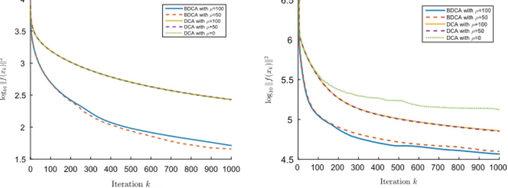
Fig. 3 Comparison of the rate of convergence of DCA (Algorithm 1) withρ ∈ {0,100}and BDCA (Algorithms 2 and 3) withρ=100 for finding a steady state of the “Ecoli_core” model (m=72,n=94)

Fig. 4 Comparison of the rate of convergence of DCA and BDCA (Algorithm 3) for finding a steady state

for different values of the parameterρ. On the left we show the “iJO1366” model (m=1655,n=2416). On the right we show the human metabolism model “Recon205_20150128” (m=4085,n=7400) [25]

16GB RAM, under Windows 8.1 64-bit. The subproblems (Pk) were

approxi-mately solved using the function fminunc withoptimoptions(’fminunc’, ’Algorithm’, ’trust-region’, ’GradObj’, ’on’, ’Hessian’, ’on’, ’Display’, ’off’, ’TolFun’, 1e-8, ’TolX’, 1e-8).

In Table 1 we report the numerical results comparing DCA and BDCA with quadratic interpolation (Algorithm 3) for 14 models arising from the study of sys-tems of biochemical reactions. The parameters used wereα=0.4,β =0.5,λ¯ =50 andρ=100. We only provide the numerical results for Algorithm 3 because it nor-mally gives better results than Algorithm 2 for biochemical models, as it is shown in Fig.3. In Fig.4we show a comparison of the rate of convergence of DCA and BDCA with quadratic interpolation for two big models. In principle, a relatively large value of the parameterρ could slow down the convergence of DCA. This is not the case here: the behaviour of DCA is usually the same for values ofρbetween 0 and 100, see

Figs.3and4(left). In fact, for big models, we observed that a value ofρbetween 50 and 100 normally accelerates the convergence of both DCA and BDCA, as shown in Fig.4(right). For these reasons, for the numerical results in Table1, we applied both DCA and BDCA to the regularized versiong(x)−h(x)withg(x)= f1(x)+100₂ x2

andh(x)= f2(x)+100₂ x2, where f1and f2are given by (30).

6 Concluding remarks

In this paper, we introduce two new algorithms for minimising smooth DC func-tions, which we termBoosted Difference of Convex function Algorithms (BDCA). Our algorithms combine DCA together with a line search, which utilises the point generated by DCA to define a search direction. This direction is also employed by Fukushima–Mine in [7], with the difference that our algorithms start searching for the new candidate from the point generated by DCA, instead of starting from the previous iteration. Thus, our main contribution comes from the observation that this direction is not only a descent direction for the objective function at the previous iteration, as observed by Fukushima–Mine, but is also a descent direction at the point defined by DCA. Therefore, with the slight additional computational effort of a line search one can achieve a significant decrease in the value of the function. This result cannot be directly generalized for nonsmooth functions, as shown in Remark1. We prove that every cluster point of the algorithms are stationary points of the optimisation problem. Moreover, when the objective function satisfies the Łojasiewicz property, we prove global convergence of the algorithms and establish convergence rates.

We demonstrate that the important problem of finding a steady state in the dynamical modelling of systems of biochemical reactions can be formulated as an optimisation problem involving a difference of convex functions. We have performed numerical experiments, using models of systems of biochemical reactions from various species, in order to find steady states. The tests clearly show that our algorithm outperforms DCA, being able to achieve the same decrease in the value of the DC function while employing substantially less iterations and time. On average, DCA needed five times more iterations to achieve the same accuracy as BDCA. Furthermore, our implemen-tation of BDCA was also more than four times faster than DCA. In fact, the slowest instance of BDCA was always at least three times faster than DCA. This substantial increase in the performance of the algorithms is especially relevant when the typical size of the problems is big, as is the case with all realistic biochemical network models.

Acknowledgements The authors wish to thank Christian Kanzow for pointing out Remark3, and Aris

Daniilidis for his helpful information on the Łojasiewicz exponent. The authors are also grateful to an anonymous referee for their pertinent and constructive comments.

Open Access This article is distributed under the terms of the Creative Commons Attribution 4.0

Interna-tional License (http://creativecommons.org/licenses/by/4.0/), which permits unrestricted use, distribution, and reproduction in any medium, provided you give appropriate credit to the original author(s) and the source, provide a link to the Creative Commons license, and indicate if changes were made.

References

1. Absil, P.A., Mahony, R., Andrews, B.: Convergence of the iterates of descent methods for analytic cost functions. SIAM J. Optim.16(2), 531–547 (2005)

2. Artacho Aragón, F.J., Fleming, R.M.T.: Globally convergent algorithms for finding zeros of duplomonotone mappings. Optim. Lett.9(3), 569–584 (2015)

3. Attouch, H., Bolte, J.: On the convergence of the proximal algorithm for nonsmooth functions involving analytic features. Math. Program.116(1–2), 5–16 (2009)

4. Bolte, J., Daniilidis, A., Lewis, A.: The Łojasiewicz inequality for nonsmooth subanalytic functions with applications to subgradient dynamical systems. SIAM J. Optim.17(4), 1205–1223 (2007) 5. Bolte, J., Sabach, S., Teboulle, M.: Proximal alternating linearized minimization for nonconvex and

nonsmooth problems. Math. Program.146(1–2), 459–494 (2013)

6. Collobert, R., Sinz, F., Weston, J., Bottou, L.: Trading convexity for scalability. In: Proceedings of the 23rd International Conference on Machine Learning, pp. 201–208. ACM (2006)

7. Fukushima, M., Mine, H.: A generalized proximal point algorithm for certain non-convex minimization problems. Int. J. Syst. Sci.12(8), 989–1000 (1981)

8. Gevorgyan, A., Poolman, M.G., Fell, D.A.: Detection of stoichiometric inconsistencies in biomolecular models. Bioinformatics24(19), 2245–2251 (2008)

9. Huang, Y., Liu, H., Zhou, S.: A Barzilai–Borwein type method for stochastic linear complementarity problems. Numer. Algorithms67(3), 477–489 (2014)

10. Le Thi, H.A., Pham Dinh, T.: The DC (difference of convex functions) programming and DCA revisited with DC models of real world nonconvex optimization problems. Ann. Oper. Res.133(1–4), 23–46 (2005)

11. Le Thi, H.A., Pham Dinh, T.: On solving linear complementarity problems by DC programming and DCA. Comput. Optim. Appl.50(3), 507–524 (2011)

12. Le Thi, H.A., Pham Dinh, T., Muu, L.D.: Numerical solution for optimization over the efficient set by D.C. optimization algorithms. Oper. Res. Lett.19(3), 117–128 (1996)

13. Le Thi, H.A., Huynh, V.N., Pham Dinh, T.: Convergence analysis of DC algorithm for DC programming with subanalytic data. Ann. Oper. Res. Technical Report, LMI, INSA-Rouen (2009)

14. Lee, J.D., Sun, Y., Saunders, M.A.: Proximal Newton type methods for minimizing composite func-tions. SIAM J. Optim.24(3), 1420–1443 (2014)

15. Li, G., Pong, T.K.: Douglas–Rachford splitting for nonconvex optimization with application to non-convex feasibility problems. Math. Progr.159(1), 371–401 (2016)

16. Łojasiewicz, S.: Ensembles semi-analytiques. Institut des Hautes Etudes Scientifiques, Bures-sur-Yvette (Seine-et-Oise), France (1965)

17. Mine, H., Fukushima, M.: A minimization method for the sum of a convex function and a continuously differentiable function. J. Optim. Theory Appl.33(1), 9–23 (1981)

18. Moudafi, A., Mainge, P.: On the convergence of an approximate proximal method for DC functions. J. Comput. Math.24(4), 475–480 (2006)

19. Nesterov, Y.: Gradient methods for minimizing composite functions. Math. Program.140(1), 125–161 (2013)

20. Nocedal, J., Wright, S.J.: Numerical optimization. In: Mikosch, T.V., Resnick, S.I., Robinson, S.M. (eds.) Springer Series in Operations Research and Financial Engineering, 2nd edn. Springer, New York (2006)

21. Parks, H.R., Krantz, S.G.: A Primer of Real Analytic Functions. Birkhäuser, Basel (1992)

22. Pham Dinh, T., Le Thi, H.A.: A DC optimization algorithm for solving the trust-region subproblem. SIAM J. Optim.8(2), 476–505 (1998)

23. Pham Dinh, T., Souad, E.B.: Algorithms for solving a class of nonconvex optimization problems. Meth-ods of subgradients. In: Hiriart-Urruty, J.-B. (ed.) FERMAT Days 85: Mathematics for Optimization, Volume 129 of North-Holland Mathematics Studies, pp. 249–271. Elsevier, Amsterdam (1986) 24. Schnörr, C., Schüle, T., Weber, S.: Variational reconstruction with DC-programming. In: Herman, G.T.,

Kuba, A. (eds.) Advances in Discrete Tomography and its Applications, pp. 227–243. Springer, Berlin (2007)

25. Thiele, I., et al.: A community-driven global reconstruction of human metabolism. Nat. Biotechnol.