CLUSTERnGO: a user-defined modelling platform for two-stage clustering of time-series data

(1)

Gene expression

CLUSTERnGO: a user-defined modelling

platform for two-stage clustering of time-series

data

Is

ık Barıs

Fidaner

1

, Ayca Cankorur-Cetinkaya

2,3,†

, Duygu Dikicioglu

2,3,†

,

Betul Kirdar

2

, Ali Taylan Cemgil

1

and Stephen G. Oliver

3,

*

1

Department of Computer Engineering,

2

Department of Chemical Engineering, Bogazici University, Istanbul, Turkey

and

3

Cambridge Systems Biology Centre and Department of Biochemistry, University of Cambridge, Cambridge, UK

*To whom correspondence should be addressed.

†_{Present address: Department of Biochemistry, University of Cambridge, Sanger Building, 80 Tennis Court Road,}

Cambridge CB2 1GA, UK Associate Editor: Janet Kelso

Received on March 3, 2015; revised on June 30, 2015; accepted on September 3, 2015

Abstract

Motivation:

Simple bioinformatic tools are frequently used to analyse time-series datasets

regard-less of their ability to deal with transient phenomena, limiting the meaningful information that may

be extracted from them. This situation requires the development and exploitation of tailor-made,

easy-to-use and flexible tools designed specifically for the analysis of time-series datasets.

Results:

We present a novel statistical application called CLUSTERnGO, which uses a model-based

clustering algorithm that fulfils this need. This algorithm involves two components of operation.

Component 1 constructs a Bayesian non-parametric model (Infinite Mixture of Piecewise Linear

Sequences) and Component 2, which applies a novel clustering methodology (Two-Stage

Clustering). The software can also assign biological meaning to the identified clusters using an

appropriate ontology. It applies multiple hypothesis testing to report the significance of these

en-richments. The algorithm has a four-phase pipeline. The application can be executed using either

command-line tools or a user-friendly Graphical User Interface. The latter has been developed to

address the needs of both specialist and non-specialist users. We use three diverse test cases to

demonstrate the flexibility of the proposed strategy. In all cases, CLUSTERnGO not only

outper-formed existing algorithms in assigning unique GO term enrichments to the identified clusters,

but also revealed novel insights regarding the biological systems examined, which were not

uncovered in the original publications.

Availability and implementation:

The C

þþ

and QT source codes, the GUI applications for

Windows, OS X and Linux operating systems and user manual are freely available for download

under the GNU GPL v3 license at http://www.cmpe.boun.edu.tr/content/CnG.

Contact:

[email protected]

Supplementary information:

Supplementary data

are available at

Bioinformatics

online.

1 Introduction

High-throughput technologies in the life sciences generate massive amounts of information by allowing the measurement of thousands

of entities simultaneously. However, understanding the underlying biological information and drawing meaningful results from such huge data sets is a challenge. Clustering is among the most

VC_{The Author 2015. Published by Oxford University Press.} 388

This is an Open Access article distributed under the terms of the Creative Commons Attribution License (http://creativecommons.org/licenses/by/4.0/), which permits unrestricted reuse, distribution, and reproduction in any medium, provided the original work is properly cited.

doi: 10.1093/bioinformatics/btv532 Advance Access Publication Date: 26 September 2015 Original Paper

at University of Cambridge on April 28, 2016

http://bioinformatics.oxfordjournals.org/

(2)

commonly employed approaches in the analysis of such data and it attempts to identify entities with similar patterns of occurrence while aiming to reveal the functional relationships between those entities.

A number of algorithms have been developed for clustering ana-lyses and their applicability is highly dependent on experimental de-sign, and investigators not infrequently select a less than optimal clustering algorithm with which to analyse their data. Such a choice may result in an inadequate or even misleading, interpretation of the outcome of a given experiment.

Traditional clustering algorithms, such as hierarchical clustering (Eisenet al., 1998), k-means clustering (Tavazoieet al., 1999) and self-organizing maps (Tamayoet al., 1999) are highly applicable heuristic methods (Yeunget al., 2001), which are very suitable for non-dynamic experimental designs. A major drawback to these methods when applied to time-series data is that they take no ac-count of the fact that successive samples in the series are related to one another. Instead, they consider the data from each successive sample as being independent from the data from all of the other samples in that time-series, and thus ignore important information.

Several clustering algorithms have been specifically designed to analyse time-series datasets. Some of these approaches utilize fea-ture-based similarity instead of point-wise similarity (Phanget al., 2003;Sahooet al., 2007). Although transforming expression pro-files into feature vectors prior to clustering was reported to lead to a faster clustering algorithm through noise reduction in the raw data (Kuenzel, 2010), this methodology permits the loss of information during data transformation due to the presence of unexpected pat-terns and similarities in the data. Ramoni et al. (2002) used a Bayesian method, representing gene expression dynamics as autore-gressive equations where each expression measurement was assumed to be a linear function of the previous measurements. However, the effectiveness of autoregressive models decreases when the time-series data are non-uniformly sampled (Mo¨ller-Levet et al., 2003). Bar-Josephet al.(2003)modelled gene expression profiles using statis-tical spline estimation as continuous piecewise polynomial func-tions. This method requires the user to provide the number of desired clusters as input and it is not suitable for short time-series datasets (Liuet al., 2005).Schliepet al.(2003)used hidden Markov models (HMM) to account for the dependencies along the time axis. The shortcoming of HMMs is their ineffectiveness for non-uni-formly sampled datasets since they disregard the information on how samples are distributed (Mo¨ller-Levetet al., 2003).

In the last decade, Bayesian non-parametric models emerged as another model-based option, which allows superior model flexibility (Sammut and Webb, 2010). The most recognized Bayesian non-parametric models are infinite mixture models, which allow a poten-tially infinite number of mixture components, which can be adapted based on the supplied input. This is achieved through the use of sto-chastic processes such as the Dirichlet process (DP) or the Pitman-Yor process (PYP) as priors in the probabilistic model. Their math-ematical structure is handled by ‘constructions’ like the ‘Chinese res-taurant process’ (CRP) or the ‘stick-breaking process’. These representations allow for derivations of iterative inference methods like Gibbs samplers and Markov Chain Monte Carlo (MCMC) methods (Neal, 2000).

Medvedovic and Sivaganesan (2002)developed a gene expres-sion analysis method based on a Bayesian non-parametric model, where a Gaussian infinite mixture model (GIMM) served as the gen-erative model to represent the assumptions regarding the stochastic data generation process implicitly. A ‘complete linkage clustering’ algorithm was employed to determine the final set of clusters.

Having noted the difficulty of the problem concerned, the authors suggested the use of ‘average linkage clustering’ algorithm for mak-ing the final clustermak-ing decision in their subsequent studies (Medvedovicet al., 2004).

Qin enhanced inference on the infinite mixture model by apply-ing collapsed Gibbs samplapply-ing, which is a predictive updatapply-ing tech-nique to integrate out parameters by calculating marginal likelihoods during each iteration (Qin, 2006). The set of samples in a given gene expression profile are assumed to be independently dis-tributed in this Chinese Restaurant Cluster (CRC) algorithm. Joshi et al.extended the infinite mixture model approach to allow for the simultaneous co-clustering of genes and experiments (Joshiet al., 2008).

In our approach to time-series gene expression analysis, we have combined the strength and flexibility offered by Bayesian non-parametric methodology by developing and using an infinite mix-ture model that is tailored to a particular experimental design. Our methodology is similar to other Bayesian non-parametric methods, but our model is specific to the experimental problem. It is imple-mented in a framework that combines probabilistic inference, clus-tering, and multiple hypothesis testing.

We present here CLUSTERnGO: a robust clustering method-ology for time-series data and, associated with it, a simple, plat-form-independent user interface to improve its accessibility by experimental biologists, who play a key role in the analysis of such datasets. The methodology assumes a user-defined Bayesian non-parametric model, where each mixture component is modelled as a piecewise linear sequence (PLS) in order to capture the ‘segments’ of time points that comprise the experiment. A two-stage complete linkage clustering procedure was employed to identify the patterns in the data. Unlike its predecessors, this simple and effective ap-proach can address all of the following issues simultaneously: (i) it allows the user to construct their own model, which would integra-tively take into account both the design of the experiment and the collected data, prior to analysis, (ii) it has a deterministic clustering output, despite its probabilistic approach introduced by two-stage clustering, (iii) it takes into account the differences and the similar-ities in both the profiles and the magnitudes of expression, (iv) it is suitable for equally or unequally sampled long or short time-series datasets, (v) it does not require ana prioriknowledge or assumption on the number of clusters that will be identified at the end of the process, (vi) it allows the assignment of the same gene into different clusters, i.e. overlapping clusters, minimizing the loss of biological information hidden in the dataset introduced by two-stage cluster-ing, and (vii) it has a very friendly GUI suitable for both specialist and non-specialist users despite the rigorous computational proced-ures running in the background.

We test the applicability of our approach on three independent published biological datasets, which are different in size, the level of gene expression under investigation, the temporal experimental de-sign, the presence of replicates, as well as the level of complexity of the model organism and demonstrate that our algorithm brings sub-stantial novel insight into the systems under investigation, which was previously not reported and outperforms its predecessors in doing so.

2 Algorithm

The algorithm we propose involves a single process of clustering analysis and consists of four successive phases: configuration (CONF), inference (INF), clustering (CLUS) and evaluation (EVAL)

(3)

(Supplementary Fig. S1). Inputs and outputs of these operations fol-low successive steps in a single pipeline. The process, taken as a whole, receives an input dataset of dynamic profiles and assigns the profiles into an optimal number of clusters based on the model determined by the user as well as reporting an output of statistically significant Gene Ontology (GO) terms that characterize those clus-ters of entities, whenever applicable. In this section, we describe the functioning of each of the four phases in the CnG algorithm pipeline.

2.1 Configuration phase (CONF)

The most important feature of datasets on transitions is the depend-ence of the value of each variable on its value at the preceding time point. Therefore, it is important to account for this information dur-ing the identification of clusters of entities displaydur-ing similar behav-iour over time. Our approach involves building a model based on the experimental input as well as the initial design of the experiment to account for the dependencies between consecutive time points in dealing with transient phenomena. CONF is the phase in our algo-rithm that configures this model.

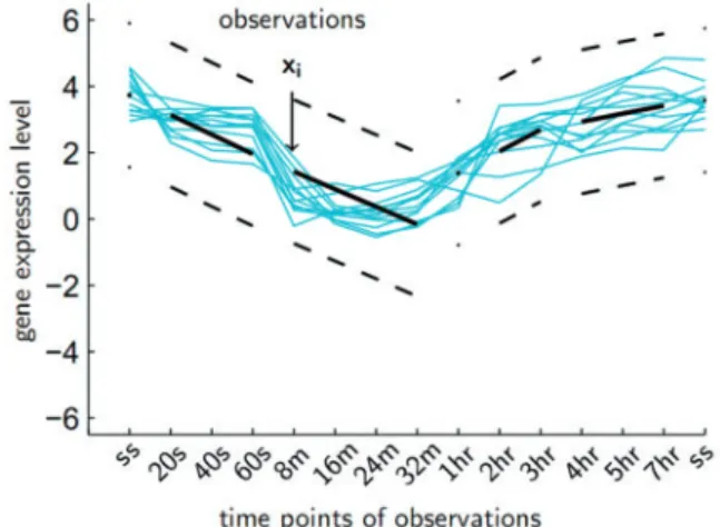
Our algorithm models the given time-series dataset by an infinite mixture of piecewise linear sequences (IMPLS). IMPLS is a special infinite mixture model whose mixture components are distributed around piecewise linear sequences (PLS). PLS assumes a particular segmentation of time points, where in each segment corresponding to a given time period, the measured level of the clustered entities is assumed to linearly increase, decrease, or constitutively stay con-stant. PLS model is illustrated inFigure 1.

CONF is the initial phase for configuring the probabilistic model for Bayesian inference. It can be configured manually by specifying a custom segmentation of time points for the PLS model, or it can be configured semi-automatically. In the semi-automatic mode, it takes the time-course profiles of the biological entities in the dataset as its input and, by applying temporal segmentation (TS) to its time points, produces the piecewise linear sequence (PLS) model that will be used in the next phase. TS has a single parameter: the segmenta-tion threshold.

TS determines which time samples show similar behaviour by taking values for each of the time points over the whole dataset, and running a standard average-linkage hierarchical agglomerative clus-tering procedure based on their pairwise Gaussian distances. By applying a threshold on the resulting dendrogram at a certain value, which we call the segmentation threshold, time samples can be

grouped such that they make up a piecewise linear sequence. The threshold is determined by the end-user in order to represent the sub-sequences of time points that are known to have a linear succes-sion in the experimental set-up as the temporal segments in the PLS model.

It is possible to trace how the groupings change as the threshold is varied, thus allowing the user to adjust the time segments until the most biologically meaningful segmentation, based on the experimen-tal design, is obtained. The constructed PLS models are then used to determine the probabilistic model in the inference phase. Although one can also take PLS segmentation as a probabilistic variable to be inferred, in CnG, we choose to keep it as a user-defined model parameter.

Biological experiments are usually designed to seek answers to specific questions and have ana priorihypothesis to be tested. This hypothesis is taken into account in the design of an experiment to determine the type and duration of the perturbations as well as the sample collection regime. In CONF, the users can construct their own models that integratively take into account both the design of experiments and the data collected from those experiments. Naturally, thea prioriexpectations arising from the initial design of the experiment may not always meet the actual outcome represented by the data generated. Thus this step may assume the role of an inte-gral checkpoint highlighting important intrinsic characteristics of the data. It may: (i) capture novel behaviour emerging from the data that was initially unexpected when designing the experiment or (ii) highlight inconsistencies or inaccuracies within the data caused ei-ther by the experiment itself or its design.

2.2 Inference phase (INF)

Following the determination of the PLS model for the given dataset in CONF, INF carries out an operation of Markov chain Monte Carlo (MCMC) probabilistic inference to obtain a pairwise similar-ity matrix. This output matrix holds the information that will be used in determining the clusters of entities. As input, INF takes the dataset and the PLS model as determined by CONF. As output, it produces the matrix of posterior pairwise probabilities.

To generate this matrix, INF runs an MCMC sampling oper-ation using four parameters: the number of chains, the number of it-erations in each chain, the number of itit-erations to be skipped, and the initial values for hyper-parameters. Following the MCMC run, the pairwise similarity matrix is computed by taking averages over all non-skipped iterations over all chains.

2.3 Clustering phase (CLUS)

After obtaining a pairwise similarity matrix by probabilistic infer-ence, we still have to determine the exact clusters of entities and apply hypothesis-testing to detect the significant GO terms associ-ated with those clusters, if applicable. CLUS is the phase that takes this matrix and applies a two-stage clustering operation to obtain clusters (subsets) of genes. This operation has two parameters as in-put: merge threshold and extension threshold, which are used in its two stages. Two-stage clustering may result in different numbers of overlapping or non-overlapping clusters depending on the given thresholds and the similarity matrix. The threshold parameters de-termine the stringency of the operation; larger thresholds will result in a larger number of clusters with fewer members, representing finer similarity relations, whereas smaller thresholds will result in a smaller number of clusters that represent coarser similarity relations. The resulting clusters are then received by the evaluation phase for hypothesis testing.

Fig. 1.An example piecewise linear sequence model

(4)

2.4 Evaluation phase (EVAL)

Multiple hypothesis testing is applied on the clusters in EVAL. This operation requires GO term assignments for all genes and an alpha parameter (a significance threshold) to use in hypothesis testing. For any given cluster, all GO terms that are directly or indirectly anno-tated with its member genes are considered as possible hypotheses. Each of these GO terms belongs to one of the three categories: cellu-lar component, molecucellu-lar function, or biological process. EVAL applies multiple hypothesis testing with Bonferroni or Benjamini-Hochberg correction for multiple testing to the whole set of hypoth-eses comprised of GO terms from all three categories, and the result-ing significant GO terms associated with each cluster are reported in the final output.

3 Implementation

3.1 CONF: temporal segmentation (TS)

TS is a simple operation where segments of time points that display a correlated behaviour are discerned by applying hierarchical ag-glomerative clustering to the vectors of values over all entities at each time point in the dataset. The resulting dendrogram is divided by a selected segmentation threshold, and the resulting sub-trees are marked as the time segments of the piecewise linear sequence model that will be used in the next phase. The PLS segmentation can also be set manually by the user (Fig. 1).

3.2 INF: MCMC for IMPLS

CLUSTERnGO (CnG) models time-course profiles using an infinite mixture of piecewise linear sequences (IMPLS). To compute the pos-terior of IMPLS, it uses an MCMC procedure.

3.2.1 The IMPLS model

Suppose that we haveNentities indexed byi2{1,. . .,N} and their profilesxi, vectors of sizeM, which are to be modelled as distributed

around an unknown number of piecewise linear sequences. Mixture component assignments zi of these entities are assumed to come

from a two-parameter CRP, an iterative construction for a PYP: z1:Nja;d CRPða;dÞ (1) A PLS model is defined byLparameters in the following order: initial value, slope of the first segment, jump to the second segment, slope of the second segment, jump to the third segment, and so on. The prior variances of these three types of parameters are given by Vinit, Vjump, Vslope. These variances form the diagonal of the

ma-trix Pm. For every mixture component k2{1,. . .,K} there is an L-vectormkthat defines a PLS with a Gaussian prior:

lkjVinit;Vjump;VslopeNðlkj0;PlÞ (2) Each cluster also has a precision (inverse variance) parameterkk

with a Gamma prior:

kk ja;bCðkkja;bÞ (3) Finally, we have the likelihood, which determines that each time-series is distributed according to a Gaussian with meanCmk

and variance 1/kk, where k is the mixture component that this

sam-ple belongs to.Cis a constant matrix that is either manually speci-fied or determined semi-automatically by the CONF procedure. This matrix transforms PLS parametersmkinto the mixture

compo-nent mean: xijl;k;ziY K k¼1 NðxijClk;kk1IÞ zik ₍₄₎

Cis a matrix of basis vectors and each time-series (here, simply a fi-nite dimensional vector) is modelled byx¼Clþe. Meanlis zero,

<l>¼0. The covariance of x is thereby <xx0_>_¼ C<ll0_>_C0_þ_R_¼_CC0_þ_R. _{The matrix} _C _{is constructed such that} typicalxare Piecewise Linear Sequencessuch sequences will have the conditional covarianceCC0_þ_R.

3.2.2 MCMC inference

A special Markov Chain Monte Carlo (MCMC) procedure was adopted in the analysis of this model due to the presence of matrix C, which transforms the parameter vector.

We run Metropolis-Hastings (MH) steps to sample the mixture component precisionskkand use these values to run collapsed Gibbs

sampling steps to sampleziby integrating out the mixture

compo-nent centresmk.Our MCMC algorithm consists of three steps

re-peatedly applied to converge to the target distributionp(x,z,k,a,d, a,b).

1. For eachk¼1. . .K, apply MH steps to re-samplekkbyp(kkj

x1:N,z1:N).

2. For eachi¼1. . .N, apply collapsed Gibbs sampling forziby

p(zijx1:N,zi,k1:K) using auxiliary variable method for sampling

newkk.

3. Apply MH steps to sample the hyper-parameters;a,d,a,bby their, respective, non-informative priors 1/a, 1/d, 1 andb. The PLS prior parametersVinit,Vjump,Vslopeare each fixed at a

sufficiently large number to assign equal probabilities for different PLS parameter values. The user is allowed to interact with the MCMC on the initial values for the IMPLS hyper-parameters, the number of iterations to be carried out, the number of chains or the skip value. The default values for the number of iterations to be car-ried out, the number of chains and the skip value for the burn-in period were set as 10 000, 20 and 2500, respectively. The number of iterations and the number of chains are kept at high values to help the MCMC inference to more closely approach its stationary distri-bution. In practice, this enables the INF phase to yield very similar results in successive runs, even though it is based on a probabilistic algorithm. The default initial settings for the hyper-parameters are as follows;a¼2.1, b¼0.24,d¼0.001 and alpha¼100 although these parameters are readjusted during the iterations.

3.3 CLUS: two-stage clustering (TSC)

CLUS is a deterministic phase where decisions are based on simple numerical comparisons on pairwise posterior probabilities. Clusters cannot be determined in the INF phase, because data is finite and there is uncertainty in the infinite mixture posterior. The CLUS phase operates on this posterior to decide on the final clusters. The inference results contained in the pairwise similarity matrix are translated into a set of clusters that indicate groups of related enti-ties through the application of a two-stage operation in the cluster-ing phase. The degree of similarity in clustercluster-ing is determined by two parameters: the merge threshold and the extension threshold.

Let M be the pairwise similarity matrix whereMijdenotes the

similarity between entity i and entity j, namely, the posterior pair-wise probabilities between these entities as obtained from MCMC. Given this matrix M and the two threshold parameters, two-stage clustering runs as follows:

(5)

1. Prepare an initial setPof 1-element clusters.

2. Choose the cluster pair (Sa,Sb) where the minimum similarity value

between anyi2Saandj2Sbis the maximum among cluster pairs.

3. RemoveSaandSb, and insert their unionSa|Sb¼Scinto the

set of clusters;P.

4. Continue from step 2 until the obtained similarity betweeni2Sa

andj2Sbis smaller than the merge threshold.

5. Choose the cluster-entity pair (Sa,j) where the minimum similarity

value between anyi2Saandjis the maximum among all pairs.

6. RemoveSaand insert its incremented setS¼Sa|{j} into the set

of clusters;P.

7. Continue from step 5 until the obtained similarity betweeni2Sa

andjis smaller than the extension threshold.

Among these steps, 2, 3 and 4 designate the first stage where small clusters are merged into larger clusters, and 5, 6 and 7 desig-nate the second stage where clusters are further extended by insert-ing elements. Intuitively, the merge threshold determines the size of cluster cores, whereas the extension threshold determines the extent of overlap among cluster peripheries. Lowering the extension threshold in stage 2 can result in wide cluster peripheries that over-lap for many genes. Lowering the merge threshold in stage 1 will yield few large cluster cores, thereby effectively constraining the pos-sibilities of overlaps in stage 2. Using this methodology, there is no need for anya prioriknowledge or assumption concerning the num-ber of clusters that will be identified at the end of the process. The default settings for the merge and the extension threshold param-eters were both 0.5, although they can be individually set by the user to any value between 0 and 1.

3.4 EVAL: multiple hypothesis testing

The identified clusters of genes are significantly associated with a biological ontology through the application of multiple hypothesis testing in EVAL. Gene Ontology (GO), where each gene is anno-tated by a list of terms from three domains: cellular component, mo-lecular function, and biological process was adopted as the biological ontology in this analysis (Ashburneret al., 2000). To de-termine if a given cluster is annotated by a given GO term at a fre-quency greater than by chance, the p-value is computed using the hypergeometric distribution: P¼1X k1 i¼0 M i NM ni N n (5)

Here,Nis the total number of unique genes,Mis the number of genes annotated by the term,nis size of the cluster, andkis the number of annotated genes in the cluster. Bonferroni correction was used as a conservative action to control the family-wise error rate. Although the Bonferroni correction is set as default, the Benjamini-Hochberg procedure is also provided as a more relaxed option to control the false discovery rate (FDR) at level alpha. The assigned GO term is identified as significant if theP-value is less than the sig-nificance threshold, whose default was set asa¼0.01.

4 Validation

4.1 Datasets

We selected three datasets, which were previously analysed using traditional clustering algorithms. Two datasets comprised non-repli-cate time series gene expression profiles with unequal sampling points. The first dataset (GLU) was generated in a study

investigating the response ofSaccharomyces cerevisiae to an im-pulse-like perturbation to remove glucose limitation from the cul-ture environment (Dikicioglu et al., 2011) and the second study (SPO) investigated how the transcriptional response varied over time shifting from spore formation (facilitated by the starvation of S. cerevisiae) to the germination of those spores induced by their transfer into rich medium (Geijeret al., 2012). Data were available att¼0, 20, 40, 60 s, 8, 16, 24, 32 min, 1, 2, 3, 4, 5, 7 and 80 h in GLU and att¼0, 4, 8, 16, 32, 48, 64, 96 and 128 min in SPO. Both studies reported a subset of genes with a differential transcriptional response (372 transcripts and 1151 transcripts for GLU and SPO, re-spectively) (File S1). The third dataset comprised of the circadian os-cillations of the proteome of Mus musculus liver cells (MUS) provided as three independent biological replicate subsets (File S1) (Robleset al., 2014) and data were available for 3089 proteins at equally sampled time points oft¼0, 3, 6, 9, 12, 15, 18, 21, 24, 27, 30, 33, 36, 39, 42 and 45 h.

4.2 Effect of parameter selection

Our clustering method (CnG) is simple enough to be used by re-searchers analysing datasets created by dynamic sampling regardless of their experience in high-throughput data analysis, yet it is suffi-ciently flexible to allow more experienced data analysts to explore their options in detail. The Bayesian non-parametric methodology permits most of the model parameters to be determined automatic-ally or integrated out analyticautomatic-ally. User-defined parameters are introduced only as needed and are intended to be kept at minimum in order to avoid an unnecessary increase in the complexity of ana-lysis. The effect of varying these parameters on the outcome of the analysis are demonstrated using the three datasets detailed in the previous sub-section.

A segmentation threshold has to be defined by the user in the CONF phase to mark the sub-trees in the resulting dendrogram as the time segments in which the values display a similar trend in be-haviour. This selection depends solely on the nature of the data, the design of the experiment, and the biological question that was sought after. The decision, therefore, has to be taking full advan-tage of the methodology to extract the most from the dataset. As the user varies the threshold, the segments formed at that threshold are visualized at the same time. This allows the user to adjust the threshold such that the biological system under investigation may be represented as realistically as possible. In the present analyses, the segmentation threshold was selected as 9 for GLU, 19 for SPO and 15.6 for MUS leading to the following segmentation profiles of (1)-(2, 3, 4)-(5, 6, 7, 8) (9)-(10, 11)-(12, 13, 14)-(15), (1, 2, 3)-(4)-(5, 6)-(7, 8, 9) and (1, 2, 3, 4, 5, 6, 7, 8)-(9)-(10 11)-(12)-(13 14 15 16), respectively. The numbers here represent the order of the time points under investigation and the brackets define the clusters that contain the indicated time-points. The similarity matrices obtained for GLU, SPO and MUS in the INF phase, which would then be used in the identification of the clusters in the next phase, had 43%, 44% and 39% of the elements with non-zero values, respectively. The convergence behaviour of our probabilistic inference method employed in the INF phase was ex-plained using the three datasets. We investigated how the number of mixture components and the hyper-parameters; a, d, a and b varied during the MCMC run. The distribution of these param-eters is given inFigures 2–c for GLU, SPO, and MUS, respectively. These histograms were computed over 7500 iterations, omitting the first 2500 burn-in iterations. The number of mixture compo-nentsK, and all the hyper-parameters;a,d, a,bare observed to

(6)

converge toward their target distributionp(x,z,k,a,d,a,b) and oscillate around their respective marginal posteriors.

The hyper-parameters (a,b) of the mixture components preci-sions (kk) converge to their respective distributions around 4.5 and

0.35 for GLU, 15 and 1.5 for SPO and 1.7 and 0.015 for MUS. The different distributions for the hyper-parametersa,bsuggest that the mixture components for the datasets are inferred to have different distributions for their precision parameterskk.Namely, in the first

and the second datasets, precisionskkare likely to be distributed

around the values 10 and 9 that carry the highest probability; whereas in the third dataset, they are likely to be distributed around the value 47 that carries the highest probability.

The other two hyper-parameters (a,d) that determine the non-parametric prior’s tendency to create more mixture components, os-cillate around (8, 0) and (7, 0) for GLU and SPO and around (19, 0) for MUS. The method infers similar hyper-parameters;a,dfor these different datasets, thus they are inferred to have similar concentra-tions in their generative process of partitioning modelled by CRP. The number of mixture components K oscillates around 31 for GLU, 37 for SPO and 101 for MUS, implying the presence of more clusters as the size of the dataset increased.

To finalise the INF phase, the information sampled in Bayesian inference is summarised in a pairwise similarity matrix to be passed on to the CLUS phase. The similarity matrices obtained for GLU, SPO and MUS had 43%, 44% and 39% of the elements with non-zero values, respectively.

The CLUS phase in the algorithm hosts the next set of user-defined parameters; the merge threshold (m) and the extension threshold (e). TSC is a simple yet powerful procedure that enables a threshold-based exploration of possible clusters of entities suggested by the similarity matrix obtained from model-based inference, with-out making any additional linearity assumptions. The merge thresh-old determines the maximum number of clusters that can be identified, whereas the extension threshold determines the max-imum extent of these clusters being identified. The final number of unique clusters depends on both of these thresholds.

We investigated how these parameters affect the clustering struc-ture by varying their values in increments of 0.1 between 0.1 and 0.9 for both the merge and the extension thresholds. We carried out these analyses on the GLU, SPO and MUS datasets (File S2, S3 and S4, respectively). Settingmto a low value allowed the clustering process to be less stringent, resulting in a few large clusters; whereas higher thresholds were associated with a more stringent clustering strategy, increasing the maximum number of clusters that can be

identified by the algorithm. The size of the dataset under investiga-tion was an important criterion in determining the total number of clusters. The number of unique clusters increased as the dataset got bigger. Furthermore, the size of the largest cluster was observed to be smaller at high e (Table 1,Fig. 3,Supplementary Fig. S2).

The merge and the extension thresholds have specific tasks in the algorithm: the former determines the number of clusters, while the latter determines the number of single-member clusters (which we will refer to as singletons). The two parameters interact in a complex manner to determine the number of clusters with a single member within the same dataset. It should be noted that, in general, a high number of singleton clusters may be an undesirable feature of any clustering application and should be avoided whenever possible.

A limited number of highly populated clusters are obtained with low values ofmande, which would be useful for highlighting the global responses of the biological system under study. However, it is also important to adjust m and e to higher values to obtain many small clusters. These may help in the identification of subsets of bio-logical entities with very similar profiles to a given perturbation, which might indicate subtly different biological responses.

We found the number of singletons to increase with increasing m and e (File S5). This increase was observed to become steeper, espe-cially in the range of 0.4–0.6 for m (Fig. 3b, f, j and d, h, l). Therefore, we adopted 0.5, the median of this range, as the default parameter setting for m in CnG. This value allows a sufficiently high number of unique clusters to be identified without allowing a high fraction of them to be populated by only one entity.

The unique clusters with two or more members are of particular interest since such clusters are suitable for annotation with biolo-gical ontologies. We therefore investigated how the number of such clusters varied with the extension threshold. The highest number of clusters with at least 2 members was obtained in the range of e val-ues of 0.3–0.6. More of these clusters would be obtained towards the lower end of this range as the datasets got bigger (Fig. 3c, g and k). We adopted a default value of 0.5 for the extension threshold, based on the results we have obtained for the three datasets under investigation. We suggest using high values for both m and e without making compromises to have an elevated fractional representation of singleton clusters and the case studies indicate the suggested de-fault of 0.5–0.5 as a reasonably safe choice. The number of clusters obtained with these settings maintains the optimal balance between having a manageable number of clusters without making substantial compromises on the extent of functional or biological annotation that could be acquired from the clustered entities in EVAL,

Fig. 2.Parameter distribution and convergence. Histograms ofK,a, d, a, bthrough the iterations for GLU (a), SPO (b) and MUS (c)

(7)

whenever applicable. However, we strongly encourage users to ex-plore their options with these two thresholds tailoring their analysis to the intrinsic nature of their experiments.

In order to further investigate the dependency between the indi-vidual cluster sizes and m and e, we have explored the entire distri-bution of cluster sizes as a function of these two parameters, at critical combinations of m and e settings; 0.1, 0.5 and 0.9. We also focused on the range around the default parameter settings and con-ducted an analysis at combinations of m and e, at 0.4, 0.5 and 0.6 (Supplementary File S6,Figs S3andS4). Our analysis indicated that the large clusters dissolved as the merge and the extension thresholds are increased, giving way to clusters with smaller size and this effect was most prominently observed in the singletons. We also observed that keeping m and e within the suggested range of 0.4–0.6 but se-lecting other settings thanm¼e¼0.5 did not yield substantial dif-ferences in the distribution of the cluster size or any compromise regarding an overshoot in the number of singletons. Our analysis indicated that these two parameters affect not only the number of singletons but the entire distribution of the cluster sizes.

We have also investigated the separation of the clusters, explor-ing the average inter- and intra-cluster distances at m and e settexplor-ings exploring the possible range of combinations of values. We have observed that the inter-cluster distance remained much higher than the intra-cluster distance for all datasets, at any selectedmande set-ting, indicating the separation between the clusters was sufficiently larger than that of the average intra-cluster variance at any selected threshold (Supplementary File S7, Fig. S5). The separation between the average inter- and intra-cluster distances was especially large for GLU and SPO, which comprised only genes that display a significant change in their expression profiles over the transition period. On the other hand, the distance between inter- and intra-cluster variances was observed to be shorter in MUS, where the significance of pro-tein expression levels was not taken into consideration.

EVAL allows the user to employ either Bonferroni correction to control the family-wise error rate or Benjamini-Hochberg procedure to control the false discovery rate (FDR) at a given confidence level in multiple hypothesis testing. Bonferroni correction was observed to yield a stricter evaluation with fewer annotations, which could be attributed to the assigned clusters regardless of the size of the dataset (File S5). The filtered GO annotation files for S. cerevisiae (gaf

version 2.0—05/04/2014) and forM. musculus(gaf version 2.0— 09/07/2014) as well as the ontology (OBO v1.2—09/04/2014) files used in the analysis were obtained from the Gene Ontology Consortium webpage (http://geneontology.org/page/download-ontology).

5 Discussion

5.1 Evaluation of the performance of CnG among

model-based clustering algorithms

The performance of CnG was evaluated by comparing the extent of biological insight gained employing this methodology to that gained by two predecessor model-based algorithms, CRC and GIMM. The default settings for CRC and CnG were used in this analysis. GIMM has a user-defined parameter setting, with no initial default value provided, and we adopted the median value for this analysis.

Initially, we carried out an internal evaluation of the clustering results to assess the quality of the set of clusters obtained from CnG in comparison to CRC and GIMM. We determined the intra-cluster tightness and inter-cluster separability based on the Davies-Boudlin index (DBI) (Davies and Bouldin, 1979), where a lower index value indicates better clustering. We computed this index for the complete range of m and e available in CnG as well as employing a range of values for the default setting of CRC and the user-defined setting of GIMM. Our results indicated that, for all test cases, the DBI of CRC algorithms varied in a very small range and the index value at its de-fault setting was equal to that of the lowest value attainable (Supplementary Table S1). CnG and GIMM both provided a wide range of DBI values across a range of parameter settings, with the DBI of CnG remaining lower than that of GIMM even at the setting that would yield the maximum value for the index, indicating higher intra-cluster similarity (distance) and lower inter-cluster similarity (dispersion). Internal evaluation schemes, although providing a val-idation on how well the clustering has performed, do not necessarily imply the best information retrieval (Manning et al., 2008). Therefore, we next analysed the extent of biological insight gained from the algorithm.

The cluster enrichments for biological process GO terms were used in the evaluation of GLU and SPO datasets in compliance with Table 1.Summary of the clustering analysis of the datasets given at the marginal parameter settings formande

Merge threshold 0.1 0.1 0.9 0.9

Extension threshold 0.1 0.9 0.1 0.9

GLU (372 transcripts) Total number of unique clusters 30 30 34 126

Size of the largest cluster 34 32 34 21

Number of singletons 2 2 2 70

Number of clusters enriched with 1þ_{GO term*} ₁₃ ₁₀ ₁₈ ₁₂

% of clusters enriched with 1þ_{GO term**} ₄₆ ₃₆ ₅₆ ₂₁

SPO (1151 transcripts) Total number of unique clusters 39 39 52 694

Number of clusters enriched with 1þ_{GO term*} ₁₄ ₁₀ ₁₆ ₃₃

% of clusters enriched with 1þ_{GO term**} ₃₆ ₂₆ ₃₁ ₂₂

MUS (3089 proteins) Total number of unique clusters 117 117 184 2249

Number of clusters enriched with 1þ_{GO term*} ₂ ₃ ₂ ₁₈

% of clusters enriched with 1þ_{GO term**} ₂ ₃ ₁ ₅

(*) indicates the number of clusters with two or more members, which are significantly enriched with at least one Biological Process GO Term (for GLU and SPO) and Molecular Function GO Term (for MUS) (P-value<0.01). (**) represents the relative percentage of clusters with two or more members.

(8)

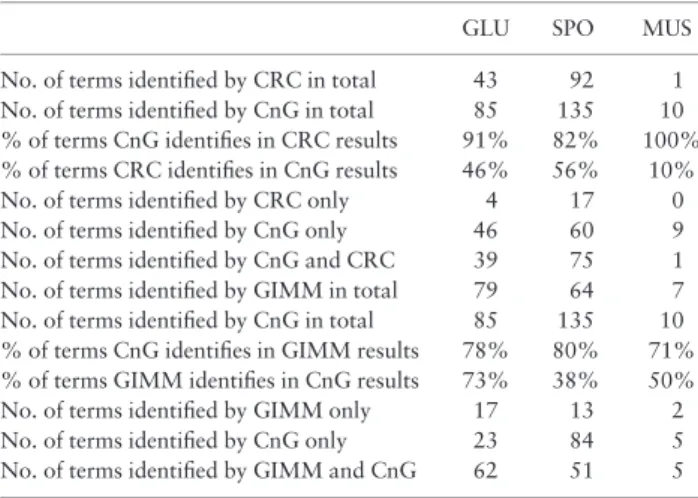
their respective publications, whereas the cluster enrichments for molecular function GO terms were evaluated for the MUS dataset, as reported. The fraction of overlap in the assignment of unique GO terms to clusters by these algorithms was inspected (Table 2). The results of this comparative analysis indicated that CnG outper-formed its predecessors in the extent of the additional biological in-formation that could be attributed to the dataset under

investigation. We then proceeded to investigate whether or not the unique GO terms identified only by CnG were only the child terms of a parent that would already be identified by the other clustering algorithm used in the comparison. The investigation of the GO terms by REVIGO (Supek et al., 2011) revealed that the pool of identified GO terms included a mixture of both newly identified terms, thus leading to novel biological information extracted from

Fig. 3.Variation in the number of clusters. The number of clusters (a, e, i), the number of singleton clusters (b, f, j), the number of clusters with two or more

mem-bers (c, g, k), and the percentage of clusters with two or more memmem-bers among the total number of clusters (d, h, l), in GLU, SPO and MUS, respectively, as a func-tion ofmandeare displayed. Both the total number of unique clusters and singletons increases asmandeget higher, whereas the percentage of clusters with two or more members among the total number of clusters begins to drop considerably at values higher than 0.6 for both m and e

(9)

the data, as well as child terms, helping to reveal more specific infor-mation from the dataset under investigation (File S8). A further in-vestigation of the expression patterns observed in the clusters that were attributed with similar functionalities by the three algorithms as well as those for which only CnG could assign functionality indicated that highly populated clusters, at times, fail to capture small clusters with specific functionality attributions and may prove problematic in capturing differences in expression profiles (Supplementary Figs S6andS7).

5.2 CnG clustering platform to get deeper biological

insight from the data

Having established that CnG extends the biological knowledge on a system considerably, we then proceeded to investigate if this new in-formation could be used in extending our understanding of the sys-tems that were under investigation by revealing novel insights. We observe that CnG identified more specific child GO terms associated with the clusters and brought novel biological insight into the ana-lysis of the experimental system under investigation in all of the three datasets.

CnG identified a group of genes whose expression was up-regu-lated in response to an impulse-like addition of glucose in the GLU dataset and associated that cluster significantly with tRNA aminoa-cylation for protein translation process of the tRNA metabolic pro-cess parent GO term. This biological propro-cess was not captured in the clustering analysis followed by ontology enrichment analysis in the respective publication. However, the publication reported an-other tRNA metabolic process, tRNA modification, to be captured through integrative analysis of the transcriptome data with tran-scriptional regulatory information.

A similar observation was made in the analysis of the SPO data-set. A cluster of genes, which were up-regulated upon the induction of germination by transferring the cells into rich, glucose-containing medium was identified and the cluster was significantly enriched with the glucose transport GO process term. Concordantly, a cluster comprised of genes that were significantly down-regulated was en-riched with the gluconeogenesis GO process term. This phenomenon of shifting towards glucose metabolism was identified via the ana-lysis of transcription factors through an integrative anaana-lysis of the transcriptome data with gene regulatory information.

These findings indicated that the fine-tuning introduced by con-structing a model for the transient behaviour of the dataset allowed clustering to capture subtle features embedded in the data, which

could otherwise only emerge through the use of elaborate integrative methods. A total of 147 unique GO terms were significantly associ-ated with the clusters identified by CnG analysis of the MUS dataset, for which 27 metabolic and cellular processes were attributed in its respective publication. In order to be able to evaluate how CnG per-forms, we focused on the 186 cyclic proteins identified in the publi-cation, for which clustering results were available.

A separate clustering analysis of these cyclic proteins revealed that more specific GO component localizations could be attributed to the proteins that vary according to the circadian rhythm of the organism. Liver proteins that were significantly associated with se-cretory granules, extracellular vesicular exosomes, blood micro-particles, and platelet alpha granules could be identified as more specific GO component terms in addition to the reported extracellu-lar space and fibrinogen complex. Furthermore, the cluster of day-time-enriched proteins was significantly associated with a novel myelin sheath GO component term. A connection between liver-associated problems (fatty liver dystrophy) and impaired nerve func-tion has long been known (Klingensporet al., 1999). The present findings indicated that there might be an additional factor intro-duced into this interconnected mechanism through the relevant pro-teins’ response to the circadian clock.

Furthermore, GO process and function terms could be attributed to the clusters populated with these cyclic proteins. The processes and the functions that were identified by CnG analysis were inclu-sive of the KEGG pathways and Uniprot Keywords discussed in the publication as well as pointing out other processes and functions, which might display cyclic responses. The cluster of daytime-en-riched proteins was significantly associated with the regulation of the ERK1 and ERK2 cascade process GO term. A previous study re-ported that the activity of Ras/ERK signalling exhibited circadian rhythms in the mouse liver clock (Tsuchiyaet al., 2013).

The clustering of the whole proteome provided as the MUS data-set revealed a cluster of 29 tightly bound proteins and two proteins in this cluster are involved in heme-copper terminal oxidase activity. Although cytochrome c oxidase subunit 6B1 was identified among the subset of proteins that were responsive to the circadian clock, cytochrome c oxidase subunit 7A2 from the same cluster, with a very similar transient expression profile, was not. The CnG analysis sug-gested the inclusion of this protein among the subset of circadian rhythmic proteins of the mouse liver cell as indicated by the analysis.

These findings indicated that CnG analysis contributed to the better understanding of the biology of the system under investiga-tion by providing novel and detailed insights regarding the dataset.

Acknowledgements

The authors thank the following members of the Cambridge Systems Biology Centre, University of Cambridge: Kathryn S. Lilley and Claire M. Mulvey, for useful discussions, and Andrew R. Hesketh, for his comments and suggestions on the GUI.

Funding

This work was supported by the Turkish State Planning Organization [DPT09K120520 to B.K.]; the Bogazici University Research Fund [10A05D4 to B.K., 08A506 to B.K., 6882-12A01D5 to A.T.C.]; TUBITAK [106M444 to B.K., 110E292 to A.T.C.], Biotechnology and Biological Sciences Research

Council [BRIC2.2 grant BB/K011138/1 to S.G.O.]; and EU 7th_Framework

Programme [BIOLEDGE Contract No: 289126 to S.G.O.]. Conflict of Interest: none declared.

Table 2.GO Term coverage performance of CnG in comparison to preceding clustering algorithms

GLU SPO MUS

No. of terms identified by CRC in total 43 92 1 No. of terms identified by CnG in total 85 135 10 % of terms CnG identifies in CRC results 91% 82% 100% % of terms CRC identifies in CnG results 46% 56% 10%

No. of terms identified by CRC only 4 17 0

No. of terms identified by CnG only 46 60 9

No. of terms identified by CnG and CRC 39 75 1 No. of terms identified by GIMM in total 79 64 7 No. of terms identified by CnG in total 85 135 10 % of terms CnG identifies in GIMM results 78% 80% 71% % of terms GIMM identifies in CnG results 73% 38% 50%

No. of terms identified by GIMM only 17 13 2

No. of terms identified by CnG only 23 84 5

No. of terms identified by GIMM and CnG 62 51 5

(10)

References

Ashburner,M.et al. (2000) Gene ontology: tool for the unification of biology.

The Gene Ontology Consortium.Nat. Genet.,25, 25–29.

Bar-Joseph,Z.et al. (2003) Continuous representations of time-series gene ex-pression data.J. Comput. Biol.,10, 341–356.

Davies,D.L. and Bouldin,D.W. (1979) A cluster separation measure.IEEE

Trans. Pattern Anal. Mach. Intell.,PAMI-1, 224–227.

Dikicioglu,D.et al. (2011) How yeast re-programmes its transcriptional pro-file in response to different nutrient impulses.BMC Syst. Biol.,5, 148. Eisen,M.B.et al. (1998) Cluster analysis and display of genome-wide

expres-sion patterns.Proc. Natl. Acad. Sci.,95, 14863–14868.

Geijer,C.et al. (2012) Time course gene expression profiling of yeast spore ger-mination reveals a network of transcription factors orchestrating the global

response.BMC Genomics,13, 554.

Joshi,A.et al. (2008) Analysis of a Gibbs sampler method for model-based

clustering of gene expression data.Bioinformatics,24, 176–183.

Klingenspor,M.et al. (1999) Altered gene expression pattern in the fatty liver dystrophy mouse reveals impaired insulin-mediated cytoskeleton dynamics. J. Biol. Chem.,274, 23078–23084.

Kuenzel,L. (2010) Gene clustering methods for time series microarray data. http://cmgm.stanford.edu/biochem218/Projects%202010/Kuenzel. Liu,H.et al. (2005) Quadratic regression analysis for gene discovery and

pat-tern recognition for non-cyclic short time-course microarray experiments. BMC Bioinformatics,6, 106.

Manning,C.D.et al. (2008)Introduction to Information RetrievalCambridge

University Press, Cambridge, UK.

Medvedovic,M.et al. (2004) Bayesian mixture model based clustering of repli-cated microarray data.Bioinformatics,20, 1222–1232.

Medvedovic,M. and Sivaganesan,S. (2002) Bayesian infinite mixture

model based clustering of gene expression profiles.Bioinformatics,18,

1194–1206.

Mo¨ller-Levet,C.S.et al. (2003) Microarray data clustering based on temporal variation: FCV with TSD preclustering.Appl. Bioinf,2, 35–45.

Neal,R.M. (2000) Markov chain sampling methods for dirichlet process mix-ture models.J. Comput. Graph. Stat.,9, 249–265.

Phang,T.L.et al. (2003) Trajectory clustering: a non-parametric method for

grouping gene expression time courses, with applications to mammary

de-velopment.Pac. Symp. Biocomput., 351–362.

Qin,Z.S. (2006) Clustering microarray gene expression data using weighted Chinese restaurant process.Bioinformatics,22, 1988–1997.

Ramoni,M.F.et al. (2002) Cluster analysis of gene expression dynamics.Proc. Natl. Acad. Sci. USA.,99, 9121–9126.

Robles,M.S.et al. (2014) In-vivo quantitative proteomics reveals a key contri-bution of post-transcriptional mechanisms to the circadian regulation of liver metabolism.PLoS Genet.,10, e1004047.

Sahoo,D.et al. (2007) Extracting binary signals from microarray time-course data.Nucleic Acids Res.,35, 3705–3712.

Sammut,C. and Webb,G.I. (eds.) (2010)Encyclopedia of Machine Learning.

Springer US, Boston, MA.

Schliep,A.et al. (2003) Using hidden Markov models to analyze gene

expres-sion time course data.Bioinformatics,19, i255–i263.

Supek,F.et al. (2011) REVIGO summarizes and visualizes long lists of gene

ontology terms.PLoS One,6, e21800.

Tamayo,P.et al. (1999) Interpreting patterns of gene expression with self-organizing maps: methods and application to hematopoietic differentiation. Proc. Natl. Acad. Sci. USA,96, 2907–2912.

Tavazoie,S.et al. (1999) Systematic determination of genetic network archi-tecture.Nat. Genet.,22, 281–285.

Tsuchiya,Y.et al. (2013) Circadian clock-controlled diurnal oscillation of

Ras/ERK signaling in mouse liver.Proc. Jpn. Acad. Ser. B Phys. Biol. Sci.,

89, 59–65.

Yeung,K.Y.et al. (2001) Model-based clustering and data transformations for gene expression data.Bioinformatics,17, 977–987.