O
|
R
|
P
|
E - A Data Semantics Driven Concurrency
Control Mechanism with Run-time Adaptation
Tim Lessner
∗, Fritz Laux
†, Thomas M Connolly
‡ ∗freiheit.com technologies gmbh, Hamburg, GermanyEmail: [email protected] †Reutlingen University, Reutlingen, Germany
Email: [email protected] ‡University of the West of Scotland, Paisley, UK
Email: [email protected]
Abstract—This paper presents a concurrency control mechanism that does not follow a ’one concurrency control mechanism fits all needs’ strategy. With the presented mechanism a transaction runs under several concurrency control mechanisms and the appropriate one is chosen based on the accessed data. For this purpose, the data is divided into four classes based on its access type and usage (semantics). ClassO(the optimistic class) implements a first-committer-wins strategy, classR(the reconcil-iation class) implements a first-n-committers-win strategy, class P (the pessimistic class) implements a first-reader-wins strategy, and class E (the escrow class) implements a first-n-readers-win strategy. Accordingly, the model is called O|R|P|E. The selected concurrency control mechanism may be automatically adapted at run-time according to the current load or a known usage profile. This run-time adaptation allows O|R|P|E to balance the commit rate and the response time even under changing conditions. O|R|P|E outperforms the Snapshot Isolation concurrency control in terms of response time by a factor of approximately 4.5 under heavy transactional load (4000 concurrent transactions). As consequence, the degree of concurrency is 3.2 times higher.
Keywords–Transaction processing; multimodel concurrency control; optimistic concurrency control; snapshot isolation; per-formance analysis; run-time adaptation.
I. INTRODUCTION
The drawbacks of existing concurrency control (CC) mech-anisms are that pessimistic concurrency control (PCC) is likely to block transactions and is prone to deadlocks, optimistic con-currency control (OCC) may experience a sudden decrease in the commit rate if contention increases. Snapshot Isolation (SI) better supports query processing since transactions generally operate on snapshots and also prevents read anomalies, but de-pending on the implementation of SI, either pessimistic or opti-mistic, it is also subject to the previously mentioned drawbacks of PCC or OCC. Semantics based CC (SCC) remedies some problems of PCC or OCC. It performs well under contention, reduces the blocking time, and better supports disconnected operations. However, its applicability is limited since data and transactions have to comply with specific properties such as the commutativity of operations. In addition to the previously mentioned drawbacks, neither PCC nor OCC nor SCC support long-lived and disconnected data processing. However, these properties are essential to achieve scalability in Web-based and loosely coupled applications. Another challenge is that in real-life scenarios often the data usage profile changes over time (e.g. stock refill in the morning, selling goods during business
hours, housekeeping during closing hours) which calls for a dynamic CC-mechanism.
This paper extends a mechanism presented in [1] and originally introduced in [2] that combines OCC, PCC, and SCC and steps away from the ‘one concurrency control mechanism fits all needs’ strategy. Instead, the CC mech-anism is chosen depending on the data usage. While the original O|R|P|E model assigns the appropriate CC-mechanism statically, this paper addresses a dynamic adaptation of the CC-mechanism due to sudden changes of the system load. To address scalability, the mechanism was designed with a focus on long-lived and disconnected data processing.
Consider, for example, the wholesale scenario as presented in the TPC-C [3]. With PCC using shared and exclusive locks, the likelihood of deadlocks increases for hot spot fields such as the stock’s quantity or the account’s debit or credit. If transactions are long-lived, PCC is even worse since deadlocks manifest during write time and a significant amount of work is likely to be lost [4] [2]. With OCC, deadlocks cannot occur. However, hot-spot fields like an account’s debit or credit would experience many version validation failures under high load causing the restart of a transaction. Like PCC, validation failures manifest during the write-phase of a transaction and a significant amount of work is likely to be lost. Both PCC and OCC cannot ensure that modifications attempted during a transaction’s read-phase will prevail during the write-phase. Whereas PCC is prone to deadlocks, OCC is prone to its optimistic nature itself.
O|R|P|E resolves these drawbacks and data can be classi-fied in CC classes. For example, customer data such as the address or password can be controlled by a PCC that uses exclusive locks only [5]. Such a rigorous measure ensures ownership of data and should be used if data is modified that belongs to one transaction. For example, account data or master data should not be modified concurrently and given the importance of this data a rigorous isolation is justified. The debit or credit of an account can be classified in CC classR, which guarantees no lost updates and no constraint violations. Such a guarantee is often sufficient for hot-spot fields. Class
E can be used to access an item’s stock, for example. Class
E is able to handle use cases such as reservations. It should be used if during the read-phase a guarantee is required that the changes will succeed during the write-phase. Class O is the default class. It avoids blocking and under normal load it
represents a good trade-off between commit and abort-rate. Section II defines these four CC classes with different data access strategies used by our mechanism. In the case of a conflict, class O implements a first-committer-wins strat-egy, class R implements a first-n-committers-win strategy, class P implements afirst-reader-winsstrategy, and class E
implements a first-n-readers-win strategy. The number n is determined by the semantics of the accessed data, e.g., by database constraints. According to the classes, the mechanism is called O|R|P|E. The “|” indicates the demarcation between data.
Section III proofs the correctness of the model. Section IV briefly describes the prototype implementation. Section V highlights some advantages of O|R|P|E, because it provides an application flexibility in choosing the best suitable CC mechanism and thereby significantly increases the commit rate and outperforms optimistic SI. The run-time adaptation mechanism and its adaptation rules are presented in Section VII. In the following Section V a prototype implementation is tested with various workloads. The results are discussed and the behavior is illustrated with time diagrams. Section VIII summarizes related work and compares it to our model. Finally, the paper draws some conclusions and provides an outlook (see Section IX) to future work.
II. MODEL
The model relies on disconnected transactions and 4 CC classes, which are defined in the following.
A. Transaction
To support long-lived and disconnected data processing, which both supports scalability, O|R|P|E models a transaction as a disconnected transactionτ, with separate read- and write-phase, i.e., no further read after the first write operation (see Definition 1, taken from [2]). To disallow blind writes, O|R|P|E guarantees that in addition to the value of a field, the version of a data field has to be read, too.
DEFINITION1: Disconnected Transaction:
1) Let ta be a flat transaction that is defined as a pair
ta= (OP, <)whereOP is a finite set of steps of the formr(x)or w(x)and<(⊆OP ×OP)is a partial order.
2) A disconnected transaction τ = (T AR, T AW)
consists of two disjoint sets of transactions.
T AR = {taR
1, . . . , taRi } to read and T AW =
{taW1 , . . . , taWj }to write the proposed modifications back.
3) A transaction has to read any data itemxbefore being allowed to modify x(no blind writes).
4) If a transaction only reads data it has to be labeled as read only.
B. CC Classes
Class O is the default class and is implemented by an optimistic SI mechanism, which is advantageous since reads do not block writes and non-repeatable or phantom phenomena do not happen. However, SI is not fully serializable [6] [7].
As stated, the drawback of optimistic mechanisms prevails if load increases, because many transactions may abort during their validation at commit time. An abort at commit time is
expensive, because significant amount of work might be lost. A circumstance particularly crucial for long-lived transactions (see [2]).
Regarding the strategy, optimistic SI follows a “first-committer-wins” semantics revealing another drawback of O. It is the lack of an option allowing a transaction to explicitly run as an owner of some data. Consider, for example, the pri-vate data of a user such as its password or address. A validation failure should be prevented by all means, since it would mean that at least two transactions try to concurrently update private data. Although technically this is a reasonable state, for this kind of data a pessimistic approach that acquires all locks at read time is more appropriate. Such a mechanism follows a “first-reader-wins” (ownership) semantics and directly leads to class P. The acquisition of exclusive locks at read time prevents deadlocks during write time. To prevent deadlocks at all, a strict sequential access and preclaiming (all locks appear before the first read) or sorted read-sets are possible mechanisms. Which mechanism is chosen to prevent or resolve deadlocks is unimportant regarding the correctness of O|R|P|E (see Section III). Preclaiming has its drawbacks concerning the time a lock has to be acquired. Sorted read-sets may be unfeasible due to limitations of the storage layer or chosen index structure. The prototype (see Section IV) uses a Wait-For-Graph to prevent deadlocks during the read-phase of a transaction. Also, during our experiments (see Section V) the number of deadlocks was considerably small, because data classified in P should have no concurrent modifications by definition.
The decision if a data item is classified asOorP is based on the following properties [2]:
1) Mostly read (mr): Is the data item mostly read? If ’Yes’, there is no need for restrictive measures and the data item should by classified for optimistic validation. A low conflict probability is assumed. 2) Frequently written(f w): f wis the opposite ofmr. 3) unknown (un): It means neither mr nor f w apply,
i.e., it is unknown whether an item is mostly read or written or approximately even.
4) Ownership (ow): if accessing a data item should explicitly cause the transaction to own this item for its lifetime?
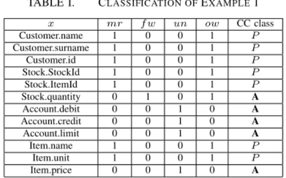
EXAMPLE 1: Classify data items in class O and P (taken from [2]).
This example is based on the TPC-C [3] benchmark and its “New-Order” transaction. Note that an additional table Account has been introduced to keep track about a customer’s bookings (column debit and credit). It also defines an over-draft limit (column limit). The following tables are used in our example: Customer (id, name, surname), Stock (StockId, ItemId, quantity), Account (AcctNo, debit, credit, limit), and Item (ItemId, name, unit, price). Table I shows an initial classification.
Attributes name, surname, and id of a customer are ex-pected to be mostly read, but if modified by a transaction it should definitively be the owner. Theidof a customer, like all ids, is expected to become modified rarely. If the idbecomes modified, ownership is required. In principal, all business keys should be classified in P, because they are owned by the application provider (see Rule 1, 1)).
Stock.quantity is expected to become modified frequently (f w) and to prevent the situation where an item was marked as available during the read phase, but at commit time the item is no longer available due to concurrent transactions, it is also marked as ow. For the time being, however, quantity will be classified as an ambiguity (see also Rule 1, 3)), which will be discussed below.
The Account.credit andAccount.debit of a customer’s ac-count might be accessed frequently depending on a customer’s activity and un is a good choice. However, since multiple transactions might concurrently update the balance, and an owner is hardly identifiable, ¬ow is chosen. So, it is also an ambiguity (see Rule 1, 3)).
TheAccount.limit is the overdraft limit of a customer and expected to be mostly read, hence,mris a good choice. Since it is neither owned by the customer nor by others, ¬ow is a good choice (see Rule 1, 2)).
Assuming the application is a high frequency trading application, Item.Price might quickly become a bottleneck. An exact prediction is not possible though, hence, un is a good choice. Propertyowwould not be a good choice, because transactions of different components (dc) might simultaneously calculate the price (see Rule 1, 3)).
TABLE I. CLASSIFICATION OFEXAMPLE1 x mr f w un ow CC class Customer.name 1 0 0 1 P Customer.surname 1 0 0 1 P Customer.id 1 0 0 1 P Stock.StockId 1 0 0 1 P Stock.ItemId 1 0 0 1 P Stock.quantity 0 1 0 1 A Account.debit 0 0 1 0 A Account.credit 0 0 1 0 A Account.limit 0 0 1 0 A Item.name 1 0 0 1 P Item.unit 1 0 0 1 P Item.price 0 0 1 0 A
The ambiguitiesA of Example 1, see class A in Table I, highlight that classes O and P and their properties are not sufficient. Particularly, hot spot items such as Stock.quantity would benefit from a CC mechanism that allows many winners and resolves the drawbacks of OCC and PCC.
Laux and Lessner [8] propose the usage of a mecha-nism that reconciles conflicts –class R–. Their approach is an optimistic variant of O’Neil’s [9] Transactional Escrow Method (TEM). Both approaches exploit the commutativity of write operations. If operations commute, it is irrelevant which operation is applied first as long as the final state can be calculated (see [8] [2] for further details) and no constraint is violated.
Unlike TEM, the reconciliation mechanism requires a dependency function. Consider, for example, two transactions that update an account and both read an initial amount of 10e, one credits in 20eand the other debits 10e. Once both have committed, it is relevant that no constraint was violated at any time and the final amount has to be 20e. Usually, a database would write the new state for each transaction causing a lost update. A dependency function would actually add or subtract the amount (the delta!) and would always take the latest state as input. In other words, reconciliation replays the operation in case of a conflict. However, this is only possible
if no further user input is required. In the example above this means the user wants to credit 20e(or debit 10e) independent of the account’s amount as long as no constraint is violated! Another requirement is that each dependency function has to be compensatable (see also [2]).
The reconciliation mechanism [8] follows a “first-n-committers-win” semantics and the number of winners n
is solely determined by constraints. The correctness of the mechanism is proven in [8], which also introduces “Escrow Serializability”, a notion for semantic correctness.
TEM grants guarantees to transactions during their read-phase. For example, a reservation system is able to grant guarantees to a transaction about the desired number of tickets as long as tickets are available. The consequence is that transactions need to know their desired update in advance (see [9] for further details).
Whereas TEM [9] is pessimistic (constraint validation during the read phase) and works for numerical data only, Reconciliation [8] is optimistic (constraint validation during the write phase) and works for any data as long as a depen-dency function is known. The proof thatE, likeR, is escrow serializable can be found in [2].
The decision if an item is member ofR orE is based on the following properties:
1) con: Does a constraint exist for this data item? 2) num: Is the type of the data item numeric?
3) com: Are operations on this data item commutative? 4) dep: Is a dependency function known for an operation
modifying the data item?
5) in: Is user input independence given for an operation modifying the data item?
6) gua: Is a guarantee needed that a proposed modifi-cation will succeed?
RULE1: Derivation of CC classes for data itemx
1) ow→classifyxinP (identify P). 2) ¬ow∧mr→ classifyxinO (identify O).
3) all other combinations of ow andmr: classify xin
A (ambiguity).
4) com→classifyxinE∨R
a) (con∧num∧com∧gua)→ classify xin
E (identify E).
b) (in∧dep∧com)→classifyx∈R(identify
R).
5) x∈A→itemxwill be eventually in O.
EXAMPLE2(Classification of data items in R and E):The ambiguities of Table I are the input for this example. Table II shows the result of the classification of these ambiguities. Stock.quantity has a constraint value > 0 and is numeric. The dependency function dep is known too. As stated above, a dependency function performs a context de-pendent write. For example, dependency function d would be d(x, xread, xnew) = x+ (xnew −xread). User input independence inis not given. If placing the order fails at the end, a replay would also fail. So, class R is not an option. Since an order requires a guarantee that the requested amount of items remains available, Rule 1, 4a) applies.
Account.creditandAccount.debitare classified as R. Property dep is known, because operations are either
TABLE II. ILLUSTRATIVE CLASSIFICATION OF AMBIGUITIES OF EXAMPLE1.
x con com num dep in gua CC class
Stock.quantity 1 1 1 1 0 1 E
Account.credit 1 1 1 1 1 0 R
Account.debit 1 1 1 1 1 0 R
Item.price 0 0 1 1 0 0 O
additions or subtractions. Propertyinis given, because the ac-count has to be updated if the order is placed and no constraint is violated. As the updates follow a dependency function they can be reconciled and should not raise an exception. Again, only a constraint violation such as an overdraft can cause the abort. Rule 1, 4b) applies.
Item.pricedepends on a variety of parameters includ-ing the last price itself. As a result, a price update might not be commutative. Item.priceremains ambiguous and remains inO, because O is the default class. Rule 1, 5) applies.
III. CORRECTNESS
A transaction potentially runs under four different CC mechanisms. Due to the CC classes’ individual semantics, each class has a different notion for a conflict, too. In any case, two read operations are never in conflict because read operations do not alter the database state and hence are commutative [10]. Usually, a conflict is given if two operations access the same data item and the corresponding transaction overlap in their execution time, and at least one operation writes the data item [5]. Whereas forO andP this is a correct definition of a conflict, forRandEit is not, because both can resolve certain write conflicts. The resolution of conflicts is a key aspect and advantage of SCC, and SCC questions the seriousness of a conflict. In other words, the meaning of a read-write or write-write conflict is interpreted. For R and E only a constraint violation is a conflict. Moreover, the state read by an operation is assumed to be irrelevant, otherwise commutativity is not given. It follows that any final serialization graphSG−Rand
SG−E for class R and E is non-cyclic because potential conflicts are reconciled (see [2] for a thorough discussion).
ForP, the common definition of a conflict is correct. If a transaction wants to modify itemp(letp∈P), it has to acquire a lock on p during its read-phase to become the exclusive owner. If not, the transaction does a blind write, which is disallowed according to Definition 1. Hence, every write in
P cannot encounter a concurrent write or read, because if a transaction writes pit has to be the exclusive owner ofP.
Consider the following (incorrect) schedule, for example (disci anddiscj denote the disconnect phase of transactioni
(resp.j) and leto∈O andp∈P):
ri(o), rj(p), rj(o), discj, wj(o), cj, ri(p), disci,
wi(p), ci (1) In this schedule transaction i readso beforej modifies o
and transaction j reads p (rj(p)) before i writes p (wi(p)).
Usually, the ordering of transaction operations are visualized by a precedence graph as in Figure 1.
DEFINITION2(Serialization Graph (SG)):LetS be a sched-ule of transactions. The Serialization Graph (aka Conflict Graph) is a precedence graph where each node represents a
transaction and each directed edge between two transactions represents a precedence of conflicting operations [11] [12] on a data item.
It is well known that a transaction schedule is conflict serializable if and only if the SG is acyclic [11] [13]. If the SG of a transaction schedule includes a cycle then no equivalent serial schedule exists and, therefore, this schedule is not serializable [11].
The above Schedule 1 leads to the following cyclic SG of Figure 1.
Figure 1. The cyclic serialization graph from Schedule (1).
Transactioniprecedesjin class Oandj precedesiinP. Having opposite orders, i.e.,i→jin one, butj→iin another class violates serializability, because globally i precedes j, which in turn precedes i.
A transaction that reads a data item in O has to validate the value at write-time, even if the write is only for an item
p∈P. The operationwi(p)causes a validation failure on item
obecause transactionihas read a value ofothat transactionj
has meanwhile updated. This is a conflict between transactions
i and j in O and produces a validation failure. Commit ci
is wrong in the schedule above and would never happen in O|R|P|E. Hence, the above schedule looks as follows in O|R|P|E:
ri(o), rj(p), rj(o), discj, wj(o), cj, ri(p), disci,
wi(p), ai (2) Even a deadlock in P cannot create a cyclic graph betweenO
andP, because at least a write is required to create a conflict in P. However, since all deadlocks can only happen during the read phase of a transaction, no conflict cycle involving a deadlock can happen in P.
Based on these initial findings it is possible to state Theorem 1. The corresponding proof exploits that for R, P, andE the corresponding serialization graphs are non-cyclic. THEOREM1: LetSG−Gbe the global serialization graph, which is the union ofSG−O,SG−R,SG−P, andSG−E. The global serialization graphSG−Gis non-cyclic ifSG−O
is non-cyclic.
Proof by contradiction:
Given thattaiis serialized beforetaj(i→j)inSG−O. In
P, no other transaction can access an item inP if transaction
tai has read this item. This is the consequence of x-locks during the read-phase used in class P. The same argument applies totajas well and it is impossible to have a serialization order j → i in P. Since i and j can be arbitrarily changed there is a contradiction if i →j exists in one, andj →i in another class.SG−RandSG−Eare negligible because any conflict is finally reconciled and both serialization graphs are non-cyclic.
COROLLARY 1: SG−O sets the global serialization order for P.
If atadoes not modify data inO, thenP sets the order. If atadoes not modify data inP, thenRsets the order, because it is prone to validation conflicts as opposed toEthat already has a guarantee to succeed.
IV. PROTOTYPEREFERENCEIMPLEMENTATION OF
O|R|P|E
The prototype of O|R|P|E is not a full database system. From a fully operational database the backup and recovery functions are missing. Both functions do not functionally influence the CC mechanism. There is only a negative effect on the performance during backup or recovery. This applies in a similar way for any database management system with a single CC mechanism.
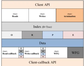
It was implemented using the JAVA programming language and Figure 2 illustrates its architecture. A client API provides access to the data and depending on the operation’s type, read or write, the operation is executed by a dedicated pool. Pools “Reads” and “Writes” represent an read- and write-lane. In addition, a pool to handle the termination (commit and abort) has been implemented. Pools’ reads and writes handle all incoming and outgoing operations and the classification has been placed directly into the index. Depending on an item’s classification the corresponding CC mechanism is plugged in. This placement allows to decide about the CC mechanism with a single read operation, which imposes an negligible overhead. Once an item has been read or written, the additional pools’ “read-callback” and “write-callback” deliver the results back to the clients. A Pool WFG (Wait-for-Graph) is used to handle access to the WFG. Deadlocks may occur during the read-phase of a transaction if the transaction accesses data items in class P. Deadlocks can only occur in class P during the read-phase, because lock acquisition is not globally ordered.
Having separate pools and callbacks to handle incoming and outgoing operations means that the prototype supports disconnected transactions, because the entire communication is asynchronous. Figure 3 illustrates the message flow within the prototype. A read operation is passed to the “Reads” pool. Each read is executed asynchronously and the complete read set is sent back to the client via a dedicated callback pool. To support asynchronous writes, a write operation is passed to the “Writes” pool and if all writes have been applied the write set is sent back to the client. Clients always sent their complete write-set.
Data is kept solely in memory and no data is written to disk unless the operating system needs to swap data to disk due to memory limitations. The only output to disk is to write logging events that are used for performance evaluation. Other functionality that has been implemented includes:
• CC mechanismsO,R,P andE, • The prototype supports constraints,
• The prototype supports item selects, range-selects, updates, and inserts. The deletion of an item is im-plemented as update that invalidates a data item.
• A WFG implementation.
Figure 2. Architecture of the prototype.
Figure 3. Message flow of the prototype.
V. PERFORMANCESTUDY WITHSTATICDATACLASS
ASSIGNMENT
The performance study has been carried out based on the prototype presented in the previous section (Section IV). As benchmark, the TPC-C++ benchmark [7] has been chosen, because we also conducted a study comparing O|R|P|E with Serializable SI, which is beyond the scope of this paper.
The data used for this study is similar to those of Examples 1 and 2. Each data item was statically assigned to a CC-Class as shown in Table III. Aspects of a dynamic assignment and its performance effects will be studied in the next section.
The performance study measures the responsetime (resp. -time), the abort rate (ab-rate), the commits per second, and the degree of concurrency (deg. conc.). The degree of concurrency is the quotient of the serial estimated execution time over the elapsed time of the experiment. In addition, the arrival rate λ
of new transactions has been varied to be set to the optimum (minimized abort rate and response time, maximized degree of concurrency). This optimum λ has been taken to conduct fair and calibrated comparisons. Each experiment has been repeated three times and the mean value is reported. Values refer to the execution of a transaction mix –deck– (42 New Order-, 42 Payment-, 4 Delivery-, 4 Credit check-, 4 Update
TABLE III. TPC-C:CLASSIFICATION OF DATA ITEMS.
Item CC Class operation
Customer P read CustomerCredit P update CustomerBalance R read Customer P read CustomerBalance R update Customer P read CustomerCredit P read StockQuantity E update Customer P read CustomerBalance R update WarehouseYTD R update DistrictYTD R update StockQuantity E read only StockQuantity E update
Stock Level-, and 4 Read Stock Level - transactions see [7] [3] [2]).
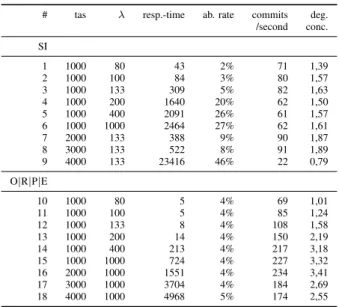
Figure 4 illustrates the abort rate and degree of concurrency for SI under full contention and shows the drawbacks of optimistic SI: the higher the number of concurrent transactions, the higher the abort rate. Also, the system starts thrashing if the degree of concurrency drops below one, which is the point where a serial execution outperforms a concurrent. Table IV shows that for SI and O|R|P|E with the same λ (tests #1-6 and #10-15) the response-time increases with largerλ, which is expected and normal behavior. The direct comparison reveals that O|R|P|E has a 3−38 times better response time, which shows that SI is over-strained for a workload ofλ≥200. For
λ = 1000 tas/sec the response time is about 3 times higher for SI and the degree of concurrency is only half compared to O|R|P|E. A good degree of concurrency with a low abort rate is given by λ= 133(see Table IV #3).
Figure 4. TPC-C++, optimistic SI (class O), abort rate and degree of concurrency.
Figure 5 shows the response-time and degree of concur-rency for O|R|P|E for increasing λ. Unlike SI, O|R|P|E has no aborts caused by serialization or validation conflicts due to the classification of hot-spot data items in R or E, which preventsww-conflicts. As shown by Figure 5, O|R|P|E has its best degree with λ= 1000transactions per second achieving 227 commits per second (see Table IV, #15).
The comparison of O|R|P|E and SI uses λ= 133 (Table
Figure 5. Response time and degree of concurrency for increasingλ for O|R|P|E .
Figure 6. TPC-C++, SI and O|R|P|E : response-time and degree of concurrency forλ= 133(SI) andλ= 1000(O|R|P|E ).
IV #3, and #7-9) for SI and λ= 1000(Table IV #15-18) for O|R|P|E . For SI,λ= 133 was considered as being the best trade-off with respect to the degree of concurrency,λ= 1000
was considered as being the best trade-off for O|R|P|E. Figure 6 illustrates the degree and the response-time for data of class O with SI and O|R|P|E if both use the λ
which reflect the best trade-off. As the figure shows, SI has a better response-time for 1000, 2000, and 3000 concurrent transactions, but then suddenly undergoes thrashing and the response-time grows exponentially. However, O|R|P|E shows a moderate and stable increase of the response-time even for 4000 concurrent transactions.
With a workload of 2000 transactions the degree of con-currency is 3.41for O|R|P|E versus 1.87for SI. The average response time is only 388 msec for SI and 1551 msec for O|R|P|E. It would be wrong to conclude that SI has a better performance than O|R|P|E because for a comparisonλhas to be taken into account. In the test O|R|P|E had a 7.5 times higher transaction arrival rate than SI (λ= 1000 as opposed to λ= 133for SI). At 4000 concurrent transactions O|R|P|E
TABLE IV. MEASURED VALUES OF EXPERIMENTS#1-18.
# tas λ resp.-time ab. rate commits deg. /second conc. SI 1 1000 80 43 2% 71 1,39 2 1000 100 84 3% 80 1,57 3 1000 133 309 5% 82 1,63 4 1000 200 1640 20% 62 1,50 5 1000 400 2091 26% 61 1,57 6 1000 1000 2464 27% 62 1,61 7 2000 133 388 9% 90 1,87 8 3000 133 522 8% 91 1,89 9 4000 133 23416 46% 22 0,79 O|R|P|E 10 1000 80 5 4% 69 1,01 11 1000 100 5 4% 85 1,24 12 1000 133 8 4% 108 1,58 13 1000 200 14 4% 150 2,19 14 1000 400 213 4% 217 3,18 15 1000 1000 724 4% 227 3,32 16 2000 1000 1551 4% 234 3,41 17 3000 1000 3704 4% 184 2,69 18 4000 1000 4968 5% 174 2,55
outperforms SI in terms of response time by a factor of3.7(see Figure 6) and the degree of concurrency is 2.6 times better. Hence, under high contention O|R|P|E has the lowest abort rate and considering the trade-off between concurrency and response time, O|R|P|E outperforms SI significantly. Further-more, its abort rate is nearly independent of the contention.
VI. RUN-TIMEADAPTION
The attempt to manually classify data may finally result in ambiguous classification where default class O applies (see Rule 1, 5)). But, high contention can quickly cause performance issues for data classified inO. Even if classP is more expensive, because P requires locking during the read-phase it will lead to a better performance in this situation as the locking will queue the transactions and process them successfully.
An automatic and dynamic adaptation of the classification when transactional load or data usage changes would make the initial classification less critical and O|R|P|E could choose the optimal CC-mechanism based on the current situation.
A solution for automatic run-time adaptation is presented in this section. It re-classifies a data items of default class
O to class P if the commit rate drops below an adjustable threshold. With this measure the commit rate increases again for the price of a longer response time. When the transactional load decreases and after the commit rate exceeds the threshold again it switches back to its original class O.
Data originally classified in P will not be re-classified to O when the load is low. This is not feasible, because an item initially in P has to remain in P due to the item’s ownership semantics. An adaption at run-time that results inO
would contradict the ownership semantics since a transaction would no longer request locks during its read-phase. This is, however, mandatory to comply with the ownership semantics (see Rule 1, 1)).
At a first glance, an adaption between E → R seems reasonable if the probability of an invariant violation (PIV) is low. It would save additional overhead, because invariant conditions in R have not to be validated at read-time, but in
Figure 7. Arrivals (workload) and time windows.
E. However, this is only a good decision if contention is low. To take this decision at high workload will result in a much longer response time because the response time for class R
grows much faster than for class E. With high contention, the probability of constraint violations increases, but the exact determination is application dependent. Classifying a data item in E is only justified if an aborted transaction is more costly than to retry the transaction, i.e., the transaction needs a guarantee to succeed which leads to classEfrom the beginning (Rule 1, 4a)).
A. Adaptation Criteria
The run-time adaptation is based on the commit rate
cr. To measure and analyze cr a statistical model for the transactional system is necessary. According to [14] [15] [16], a transactional system is modeled as an open system whose transactional arrival rate is a Poisson process. The time between arrivals of transactions is assumed to be independent in Poisson, which has the advantage that the conflict rate (the term conflict is stated more precisely below) can be modeled around a single variableλthat represents the number of arrivals in relation to the time window. A Poisson process has a conflict probability density function P Cx(X =k)given by Equation
(3):
P Cx(X=k) =λ
k
k!e
−λ (3)
For example, if on average100 transactions arrive within one Time Window (TW), the probability that k = 50 trans-actions access item x within a TW is given by Formula (3). The arrival rate λis in relation to time, for example, within one second; i.e., for a transaction that accesses x during that second, it means that the probability is P Cx(X >= 2) =
P∞
k=2λ
k/k!e−λ to encounter other conflicting concurrent
transactions.
Figure 7 illustrates the usage of TW as well as the arrivals –workload– in relation to time. The workload is, however, not constant over the lifetime of a transaction. A constant workload ignores that the workload, and hence,λmight suddenly change in particular if transactions are long running. Measuring the number of transactions terminating or committing during a time window are means to detect and react to sudden changes in the workload, which is an idea borrowed from [14]. The length of the TW defines the sample rate and its sensitivity.
The commit ratecris used as indicator for the performance of the optimistic CC-mechanism of class O. If the cr drops below a threshold, there are more aborts due to validation failures and that class P would be a better choice to increase
cr.
cr:= #committed tas/TW
(#terminated tas−#re-class. aborts)/TW (4) For each TW the commit ratecris calculated as fraction of the committed transaction divided by all terminated transaction without those that were aborted due to a re-classification. The commit rate cr is identical to the effective commit rate creff
(see Definition 5) if no adaptation occurs. Formula (4) is apparently insensitive to the length of the TW. But, a longer TW tends to compute smoother cr and it saves measuring overhead. We used a TW of100msec which delivered a good trade off for the prototype implementation.
The adaptation policy is given by Rule 2, which uses a threshold γ for the target commit rate and an hysteresis δ
to avoid constant switching (thrashing) between both classes. When a data item is re-assigned during an active transaction, the transaction is aborted when the change is from O to P. In the opposite case, the transaction can continue without conflicts, because the write-phase will succeed since the data item is already exclusively locked for that transaction. RULE2: General AdaptationO→P
Let cr be the commit rate,δ the hysteresis, and γ the target commit rate. Adaptation is according to the following rules:
1) Whencr decreases andO is the current class for an itemx: Ifcr < γ−δthenP is the new classification of x
2) Whencr increases andP is the current class for an itemx: Ifcr > γ+δthenOis the new classification of x.
3) Reclassification during a transaction:
a) If a ta reads at the time when O is the current class, but will write at a time whenP is the current class,tais aborted (non-avoidable crash) to maintain consistency.
b) If atareads at a time when the data item is inP
and writes when it is inO, the success of the write is guaranteed because the data is exclusively locked since read-time.
Adaptation solely relies on the commit ratecr. The arrival rate λ and hence the conflict probability are not measured which would be much more difficult. This leverages the deci-sion to use a Poisson distribution for the transaction arrivals.
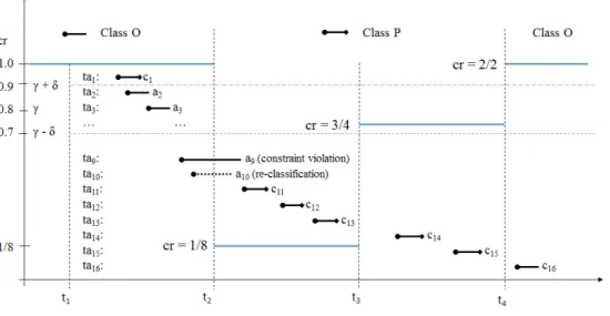
Figure 8 illustrates how the adaptation works if the commit rate decreases and later increases again. During the first TW (t2−t1) the commit ratecrdrops to1/8because only one out of 8 transactions was successful. Two transactions (ta9, ta10) have not terminated yet.
At the end of epoch 1 the commit rate is compared toγ−δ
and as cr is below the threshold dataxis re-classified to P. The transactionta9will later abort due to a constraint violation and ta10 has to abort because of the re-classification to P. Now, for the following transactions the locking mechanism for
P applies. One consequence is thatta11, ta12, andta13execute mostly sequentially. The commit rate grows in the following TW to3/4, but, this is not sufficient to switchxback to class
O. During the third TW (t4−t3) the commit rate rises to
cr= 2/2> γ+δand the (initial) optimistic CC (class O) is re-established.
The following history describes the example of Figure 8 more formally:
H = (r1(x), r2(x), r3(x), . . . , r10(x), w1(x), c1
| {z }
commit rate decreases w2(x), a2, w3(x), a3, . . .
| {z }
commit rate decreases
,adapt to P, a10, a9,
l11(x), r11(x), w11(x), c11, l12(x), r12(x),
| {z }
commit rate increases
w12(x), c12, l13(x), r13(x), w13(x), c13. . .
| {z }
commit rate increases
The history H shows in the first phase 10 trans-actions ta1, ta2, . . . , ta10 accessing x. They first read x (r1(x), r2(x), r3(x), . . . , r10(x)) and then try to write x (w1(x), w2(x), . . .). In the given scenario onlyta1can commit (c1), all others have to abort (a2, a3, . . .) because too many transactions try to concurrently update x. This leads to a sudden decrease in the commit rate cr = 1/8 because only
ta1 was successful andta9 andta10 have not yet updatedx, i.e., it is still pending. If we assume a threshold γ of 0.8 and an hysteresis δ of 0.1, then cr < γ −δ which triggers the adaption according to Rule 2, 1).
After adaptation has been carried out, ta10 has to abort (Rule 2, 3a)) if it tries to updatex. The aborta10appears in the history after the adaptation even though the itemxis now classified in P. Transactionta10 has to abort, because it has not lockedxbefore readingx(r10(x)). Ifta10would not abort it would risk a lost-update, becauseta10 would overwrite the last committed state since P does no version validation. Even with version validation, ta10 is very likely to abort, because the probability for a validation failure is high in this situation. Let assume that transactionta9accesses other data besidex and validation fails due to a constraint violation. This leads to an abort ofta9. The distinction of the abort reason is important here as it will be counted for the commit rate.
After the adaptation to P newly arriving transactions apply a locking scheme for data x which is indicated by
l11, l12, . . .. The commit rate increases again because transac-tionsta11, ta12, ta13succeed and commitc11, c12, c13. In fact, all following transaction succeed except those which violate a constraint.
If we choose the Time Window TW to start just before
ta11 arrives the commit rate cr rises with each committed transaction. Class O is not reestablished at the end of this TW despite that the next3 transactions succeed becausecr= 3/4≤γ+δ= 0.9. The class assignment remains unchanged and the following TW (t4−t3) will reestablish classObecause
cr= 2/2.
The adaptation mechanism proposed in Rule 2 maximizes the commit rate as seen in the previous example. But due to the restrictive locking policy the response time increases
Figure 8. Example run-time adaptation scenario with decreasingcrin TW(t1, t2), reclassification att2toP and increasingcrin TW(t2, t3)and(t3, t4)
and switch back to classOatt4.
as the execution tends to be serial. In the worst case, endur-ing contention, the growth is exponential. But, what if the maximum response-time is limited, for example, by Service Level Agreements (SLA) and penalties apply for exceeding the maximum acceptable response-time? The SLA penalties may outweigh the costs for aborts.
In this case maximizing the commit rate as only criteria is not a good strategy since it increases costs. To prevent unac-ceptable response times a barrier (denoted as β) is used that regulates the adaptation; i.e., onceβis reached re-classification to O takes place despite a low commit rate and the abort rate starts to increase which in turn leads to shorter response times for the remaining successful transactions. The concrete value of β is application dependent. Its general purpose is to minimize costs, i.e., if the abort costs are lower than the costs for exceeding the response-time, more aborts are acceptable until the ratio turns over.
Application specific requirements that setβ are out of the paper’s scope, but to allow applications to limit the adaptation,
β is incorporated in O|R|P|E (see Rule 3). Applications can now set β to limit the response time and, at run-time, continuously monitor and adapt the achieved commit rate as well as the response time as measured by the applications themselves. Further, applications can increase β at run-time appropriately. This way, applications can determine their own equilibrium between commit rate and response-time.
The challenge is the estimation of the expected mean response-time rtest, which implies to predict the workload.
As stated in the previous section, this is complicated if not impossible in a general and dynamic way. O|R|P|E circum-vents this problem and measures the time between a read and the corresponding write if the current classification is P. Furthermore, adaptation does no longer calculate cr at the end of the current TW, instead each termination (commit and abort) triggers the adaptation. A useful fixed TW is difficult to choose. If TW is too short, the overhead is considerable and degrades performance. If the TW is too long the adaptation is too slow.
To estimate the future workload the terminating transaction
snapshots the lock queue’s size if P is the current class. The current queue size together with the average time between read and write give a good indication for the expected workload. Because the transaction has to notify all waiting transactions about the ongoing unlock and already is the current owner of the lock-queue, there is no need for further synchronization and the overhead is considerably low, but of course exists. It is a price that has to be paid to get run-time adaptation.
Finally, the number of notified transactions multiplied by the average time distance between a read and write is used as an approximation forrtest. The rationale is that ifqtransactions
are waiting to execute and the mean time between read and write is ø(mt) then for newly arriving transactions rtest is
expected to be rtest= ø(mt)×(q+ 1)because of the mostly
sequential execution. Following this approach O|R|P|E can balance commit rate and response time.
Transaction termination triggers adaptation, however, it is important to note that the adaptation is not executed as part of a transaction. This prevents the situation where a failed adaptation would cause the transaction to abort, too.
RULE3: AdaptationO→P with barrier
Letcrbe the commit rate,δthe hysteresis,γthe target commit rate, andβ the response time barrier. Adaptation is according to the following rules:
1) (O → P): If O is the current class for an item x
and cr < γ −δ and rtest < β then P is the new
classification ofx.
2) (P →O): IfP is the current class for an itemxand
cr is low (cr < γ−δ) andrtest> β
thenO is the new classification of x.
3) (P →O): IfP is the current class for an itemxand
cr is high (cr > γ+δ)
thenO is the new classification of x. 4) Reclassification during a transaction:
a) If a ta reads at the time when O is the current class, but is about to write at a time when P is the current class, ta is aborted (non-avoidable crash) to maintain consistency.
b) If atareads at a time when the data item is inP
and writes when it is in O the success of the write is guaranteed because the data is exclusively locked since read-time.
Rule 3, 1) takes care that the commit rate is sufficiently high as long as the response time is low. If the response time exceeds the limit β and cr is (still) low then Rule 3, 2) switches back toO. Rule 3, 3) ensures that when the commit rate is high the default CC-mechanism of class O is chosen. For all other situations the classification remains unchanged.
Rule 3, 4) is the same as before. It ensures that a reclassi-fication can take place during ongoing transactions. Reclassi-fication is now triggered by two parameters, the commit rate
cr and the mean response time mrt.
VII. PERFORMANCE UNDERADAPTATION
The performance study uses the implementation of O|R|P|E described in Section IV. Even if it is not a full database implementation with all features (no backup and no recovery functionality) it is sufficient for measuring the performance of O|R|P|E under different situations. Since backup and recovery are normally inactive there is no impact on the concurrency mechanism. Therefore, the performance measurements would also be valid for a fully featured database system. Clearly, if backup or recovery are active, this would impair performance. This would also apply to our prototype.
The study analyzes different workload profiles indicated by a sequence of workloads with a total life-span of one second each. The workload is held constant for one second (called epoch). The arrival rateλ for the workload ranges from6.66
tas/sec up to a heavy overload of over300tas/sec. These values have been chosen, to show the behavior of the overloaded system with frequent aborts and the behavior under moderate workload with a stable commit rate.
During one epoch (1 sec) the commit rate is measured 10 times (sample ratesr= 10/sec). For simplicity, all transactions read and write only one data item, i.e., the worst case is simulated where an item inOsuddenly becomes a bottleneck. The time unit in all simulations is milliseconds if not stated otherwise.
To obtain a preliminary understanding the first experiments study short living transactions with no disconnect time during three epochs. Afterwards long living transactions with a ran-dom disconnect time dt between 100 and 1000 milliseconds are analyzed over seven epochs. A disconnect time dtwithin these bounds simulates typical situations.
Finally, barrierβis enabled for the next set of experiments. The set up of long living transactions and seven epochs is always the same except for the response time barrierβ which varies between1000and15000msec. We study the effects on commit rate cr and response time rt. Each experiment was executed three times.
A. Short Living Transactions with Three Epochs
Table V lists our test scenarios and summarizes the result. The right column of the table refers to the corresponding figures for a detailed analysis. The four tests use a different arrival rate λfor each epoch (one second interval) as marked in the Epochs column. The first two test scenarios do not
require a concurrency control adaptation to demonstrate the base performance without adaptation. In Tests #3 and #4 the workload is increased to trigger adaptation.
TABLE V. RESULTS FOR THREE EPOCHS WITH DIFFERENT WORKLOAD,γ= 0.9,δ= 5%ANDdt= 0.
Summary
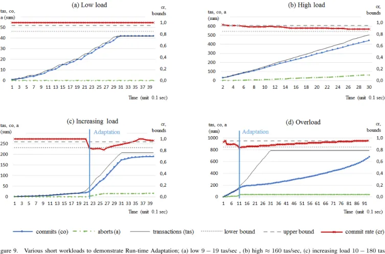
Test# Epochs ø(cr) σ(cr) ø(rt) Figure 1 9,14,19 1,00 0,00 3,6 9 (a) 2 153,176,176 0,89 0,16 2 9 (b) 3 10,19,178 0,96 0,06 3,7 9 (c) 4 168,310,309 0,90 0,05 2824 9 (d)
The average response time ø(rt) is very high for test scenario #4. This is the result of an increasing overload, which quickly triggers adaptation at the beginning of the second epoch (see Figure 9 (d)). This leads to a mostly sequential execution of the transactions, which explains the very high ø(rt)and the high ø(cr)at the same time. This increase ofcr
is typical for scenarios after adaptation to P has taken place. It continues until the upper bound γ+δis reached. Then the adaptation switches back to classO.
As the tests indicate later, it would be better to add an additional criteria for the re-adaptation from P → O. If the workload is still high (wait queue>1) the data should remain inP until the workload is low again before going back toO. This measure could avoid multiple re-adaptations that produce an unstable system behavior during a sudden transition of the workload from heavy overload to low workload.
Figure 9 shows the commit ratecr, lower and upper bounds (set by γ ±δ), and the accumulated number of aborts and commits of the four test scenarios.
Test #1 has a low workload in all three epochs. The load starts with 9 tas/sec, continues in epoch #2 with 14 tas/sec and in the last epoch the workload rises to 19 tas/sec. The transactions are executed as they arrive and no concurrent interleaving transactions occur. As expected, no adaptation takes place. From the corresponding Figure 9 (a) it can be seen that the commit rate is 1 and no aborts occur. After 3.1
sec (31 time units) all transactions have successfully terminated and the number of commits remain constant. Test #1 is the only scenario without contention but surprisingly not the shortestrt. The reason for this is that a commit is more expensive than an abort for an optimistic CC. Compared to the other tests, Test #1 has no aborts and a commit rate of 100%.
For Test #2 the load is high (≈ 160 tas/sec) and nearly constant for three seconds. The load is heavy and contention is present as can be seen from the number of aborts and the decreasing commit rate. Figure 9 (b) shows that the commit rate does not fall below the re-classification limit, hence no adaptation occurs. The data remains in class O and the optimistic CC has low overhead which results in a short response-time of only 2 msec.
Part (c) of Figure 9 (Test #3) shows the results for an increasing workload where finally in the third epoch the adaptation is triggered. The workload starts with 10 −19
tas/sec for two seconds and continues with 178 tas/sec for the third epoch. The commit rate drops under the minimum threshold (γ −δ) at the blue vertical line (2.2 sec after start). The CC-mechanism immediately switches to locking and the number of aborts decreases (the accumulated abort
Figure 9. Various short workloads to demonstrate Run-time Adaptation; (a) low9−19tas/sec , (b) high≈160tas/sec, (c) increasing load10−180tas/sec, (d) increasing overload170−310tas/sec,γ= 90%,δ= 5%,sr= 10/sec, anddt= 0.
graph makes a sharp bend to a lower gradient). During the third epoch the workload is slightly higher than the system can immediately execute. This can be seen from the slowly growing gap between the accumulated transaction arrival (tas) and the accumulated committed transactions (co). The average response time ø(rt)stays low since during the first two seconds the transactions were executed under O with shortrt.
It is interesting to compare Tests #2 and #3. Test #2 has a constant high workload, but not high enough to trigger the adaptation, hence, the data remains in O. This is the reason for the very short response time. Test #3 has initially a low workload, but in Epoch #3 the workload just exceeds the threshold and adaptation to P applies. This leads to a higher
rteven if the average workload is below the workload of Test #2.
Also, a start with low load (Tests #1 and #3) reduces the response-time because all transactions of the first epoch are executed under optimistic CC with a short rt.
Test #4 produces a heavy and increasing overload which triggers adaptation at the end of epoch 1. The gap between committed and arrived transactions grows until the arrival ends after 3 seconds. The adaptation to P allows to increase the commit rate until after 10 sec all queued transactions have terminated. The system needs 7 sec to process the queued transactions after the arrival of transactions has stopped before it becomes resilient. This explains the high mean response time ø(rt).
It can be noted that run-time adaptation under heavy
work-load achieves an average commit rate ø(cr)of approximately
90%, which was preset by γ. The price for improving cr is clearly a longer response-timertwhich grows to2.8seconds for continuous overload in test-case #4.
The commit rate cr is the basis for adaptation. When cr
drops below the lower boundγ−δthe adaptation is triggered and cr increases again. The commit rate cr increases until the upper bound γ+δ is reached which again triggers re-classification.
Summarizing, for sudden increases and decreases of cr, adaptation ensures a good response-time and a high commit rate if transactions are short lived (dt= 0) and the system is not permanently overloaded. If contention constantly remains high, adaptation has severe effects on the response-time. B. Long Living Transactions, Seven Epochs, and β disabled
Long living transactions are characterized by a certain time interval between the read phase and the write phase where no data access occurs. Some authors [17] [18] [19] [20] [21] [22] call this interval ”think time” when a typical transaction reads and displays data, then the user thinks about it, and finally modifies or adds some values. We prefer to call this time ”disconnect time”, because Web based transactional systems tend to logically disconnect from the database during this period.
For the tests a disconnect timedt from 100 - 1000 msec was randomly chosen. Each test consisted of seven epochs with different workloads. Workload W1 starts withλ= 7−14
tas/sec and rises the workload in epochs3−7from 80 tas/sec continuously to 106 tas/sec. Workload W2 stresses the system with an increasing overload from 66−460tas/sec.
The detailed workload profiles are as follows: • W1=(7,14,80,87,93,100,106) and
• W2=(66,132,200,265,332,400,460).
Each number denotes the transactions arriving during the respective Epoch of one second each. The tests were executed with two target commit ratesγ= 0.9and0.7. Table VI shows a summary of the results.
TABLE VI. RESULTS OF SEVEN EPOCHS WITH WORKLOAD W1= (7,14,80,87,93,100,106),
W2= (66,132,200,265,332,400,460),γ= (0.9,0.7),RANDOM DISCONNECT TIMEdt= 100−1000MS,AND BARRIERβDISABLED.
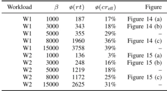
Workload γ ø(rt) #Tas ø(creff) Figure
W1 90% 4561 487 82% 10 W2 90% 24104 1845 82% 11 W1 70% 927 483 57% W2 70% 18957 1845 46% 12
Adaptation from O → P causes a systematic abort of pending transactions originating in O. To take these aborts into account the effective commit rate is defined as:
creff:=
# committed tas
# terminated tas (5)
The effective commit ratecreffmeasures -as the name
suggests-the performance of suggests-the system as shown to suggests-the user and suggests-the previously defined commit ratecris used to trigger adaptation, because this indicator is more sensitive to the workload. The effective commit rate creff reached our tests 82% for the first
and ≈ 50% for the second value of γ. Note that without adaptation all experiments would have a commit rate between 1 and 3 percent only due to the long living nature of the transactions and the higher conflict potential. This is also the reason why the performance in this test scenario is lower than in the previous subsection without disconnect time.
W1 has the shortest response-time due to the comparatively low workload. In Epoch 3 with high workload (80 tas/sec) quickly lets cr drop under the lower boundaryγ−δ= 0.85
(see Figure 10). The adaptation to P is triggered and in the following epochs cr rises again until the upper boundary is reached. The data is reclassified in O after 11 epochs and again the cr drops, but recovers faster as before, because the arrival of new transactions stopped after 7 epochs and after 12 epochs all pending transaction have terminated.
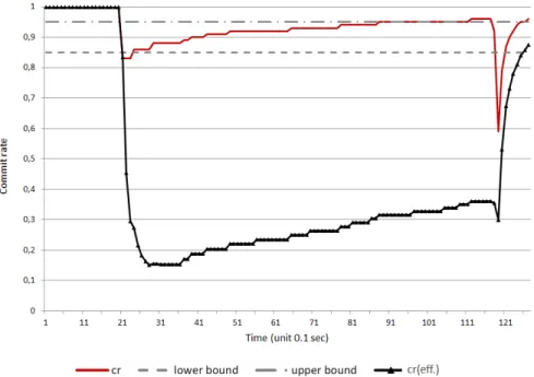
The adaptation profile for workload W2 (permanent con-tention) shown in Figure 11 is similar to W1. Due to the heavy workload starting in Epoch 1, the adaptation is already triggered at the end of Epoch 1. The permanent overload leads to a significantly longer mean response-time due to locking and queuing in P.
For workload W2 (permanent contention, second row), the mean response-time is significantly longer due to the queuing effect underP. Taking the same workload with a target commit rate of γ = 70% the adaptation behavior shows an instability (Figure 12). After adaptation to P, the upper boundary for
cr is reached very quickly during the third epoch (time = 27 units = 2.7 sec) and the data is reclassified again in O
(Rule 2, 2)) with the result that the commit rate cr drops to 40%. After this decrease, the system recovers slowly and reaches the upper boundary in epoch 14 again. At this point the arrival of transaction has already stopped but the remaining (queued) transactions cause another jitter for cr.
The reason for this oscillating effect is that Rule 2, 2) does not look at the number of queued transactions it only takes criteria cr > γ+δ to re-classify the data in O again. But in this situation all pending transactions except one will fail due to concurrency violation. This lets the commit ratecr
drop as low as 40%.
It takes now longer for the adaptation mechanism to reach the upper boundary because many transactions have already aborted and accordingly more transaction have to commit to risecr. The upper boundary is reached after 14 sec when the arrival of transaction has already stopped.
Summarizing, despite a sudden increase in contention, adaptation keeps the commit rate stable even if transactions are long living. If contention remains high, the response-time is getting longer since P queues transactions. With a low γ the mechanism tends to become unstable and an oscillating behavior can be noticed. Havingγclose to 100% is recommended since adaptation is triggered earlier. To prevent an excessive increase in response-time,β has to be enabled as discussed in the next section.
C. Long Living Transactions, Seven Epochs, and β enabled The following experiments study the effects on the work-loads of the previous subsection if barrier β is enabled andγ
is high (=90%) as recommended before. Table VII summarizes the results and shows barrier β, mean creff, and the mean
response-time ø(rt)for workloads W1 and W2. It further links to Figures 14 and 15 showing sample graphs of one run of an experiment at a time.
TABLE VII. RESULTS OF SEVEN EPOCHS WITH WORKLOAD W1= (7,14,80,87,93,100,106),
W2= (66,132,200,265,332,400,460),γ= (0.9),RANDOM DISCONNECT TIMEdt= 100−1000MS,AND BARRIERβENABLED.
Workload β ø(rt) ø(creff) Figure
W1 1000 187 17% Figure 14 (a) W1 3000 343 18% Figure 14 (b) W1 5000 355 29% – W1 8000 1960 36% Figure 14 (c) W1 15000 3758 39% – W2 1000 136 3% Figure 15 (a) W2 3000 248 16% Figure 15 (b) W2 5000 1219 18% – W2 8000 1172 25% Figure 15 (c) W2 15000 2625 31% –
As Table VII shows, each workload was executed with different values (1000,3000,5000,8000,15000) for β. All experiments show that the mean response-time is bounded by
β and the effect of a very long response-time of 19 or 24 seconds (see Table VI of the previous section’s experiments) with workload W2 no longer occurs. The table also shows that the value of β does not allow to infer the actual mean response-time. However, it shows that for an increasingβ, the response-time and the commit rate increase and β correlates with these values.
Barrier β does not directly match with the maximum response-time as given, for example, by Service Level Agree-ments (SLA). The response time depends on the workload
Figure 10. Run-time adaptation for W1= (7,14,80,87,93,100,106),γ= 0.9, random disconnect timedt= 100−1000ms, and barrierβdisabled.
Figure 11. Run-time adaptation for W2= (66,132,200,265,332,400,460),γ= 0.9, random disconnect timedt= 100−1000ms, and barrierβdisabled.
and is directly influenced by the transactions’ arrival rate. The distribution of the response time depends additionally on the concurrency model. For a queuing system like the concurrency model of class P a Poisson arrival process is assumed. The response timertis calculated as wait timewtin the queue plus transaction processing pt time. Even in the simplest queuing system, the P/P/1, with Poisson arrival and one service process, only statements about the mean response time ø(rt) can be made. To estimate the expected response timertest, the arrival
and service rate is necessary. But in the present case both rates are heavily changing. If the arrival rate would only change due to statistical variation no adaptation would be necessary. But
if a systematic change happens, e.g., because the data access type changes, the original class assignment is not any more suitable. Adaptation changes the service time and hence the service rate as well. The service time st in the case of P is the time between read and write. The only indicators for the estimated response time are the wait queue length |Qw| and
the past average ø(st). This leads to Formula (6):
rtest:= ø(st)×(|Qw|+ 1) (6)
The calculation takes into account the transactions that are already queued for execution and the average time to process
Figure 12. Run-time adaptation for W2= (66,132,200,265,332,400,460),γ= 0.7, random disconnect timedt= 100−1000ms, and barrierβdisabled.
a transaction. The processing time includes a possible waiting time due to locking.
The SLA defines a limit for the response time rt and in the case of an SLA violation, a penalty has to be paid. There is a trade off between loosing transactions or having excessive response time. Assuming an average price of r for each lost transaction and a penalty of pfor every transaction exceeding the response time limitβthe trade-off is given at the intersection of two cost functions that depend on the commit rate cr and the number of transactionstas:
ca:=r×(1−cr)×tas (7)
cp:=p×tasrt>β(cr)×tas (8) If the functions are normalized with the number of trans-actions tas then Figure 13 shows the principal graph for this trade off. The break even point for this normalized example is given at commit rate cr = 0.72. In practice, the database system will measure the actual and number of aborts and the application should monitor these values and calculate the break even based on the costs for SLA violation and failed transactions.
In the case of a fast changing workload it is difficult to estimate the workload profile. If the calculation is based on the past workload, the system may not react fast enough to sudden changes of the arrival rate.
The situation is more promising if a workload profile is known in advance. This is often the case if employees have clear routines during their workday. Assume, for example, the following tasks: order processing in the morning, stock administration after lunch, and master data management from 5 pm to 6 pm. In this scenario data access to product data in the morning and afternoon will be classified O while the product data will be re-classified to P from 5 - 6 pm.
Figures 14 and 15 illustrate the run-time adaptation profile if β is set. The time of the estimated response time rtest is
Figure 13. Example trade off between aborts and response time in terms of costs.
shown on the right vertical axis. The left ordinate shows the commit rate and the target boundaries. The horizontal axis shows the transactional time which is given by a sequence of time ordered events. The time interval from one event to the next is not constant and hence the time scale is not linear.
In Figure 14 (a) the commit ratecris1during the first two seconds when the workload is low. When the overload begins after two seconds the commit ratecr drops quickly below the lower bound γ−δ = 0.85 and adaptation to P takes place. The effective commit rate creff (green line in Figures 14 and
15) always stays below cr because cr does not count aborts due to the adaptationO→P, butcreff does. After adaptation
toP the system stabilizes the commit ratecr as shown by the red graph. This appears in all test runs and can be seen more
Figure 14. Run-time adaptation profile for target commit rateγ= 0.9: (a) workload W1 withβ= 1000, (b) Workload W1 withβ= 3000, and (c) Workload W1 withβ= 8000.
Figure 15. Run-time adaptation profile for target commit rateγ= 0.9: (a) workload W2 withβ= 1000, (b) Workload W2 withβ= 3000, and (c) Workload W2 withβ= 8000.
clearly when we have a higher response time limitβ as in part (b) and (c) of Figure 14.
In the case ofβ= 8000(part (c)) the commit rate increases until the estimated response time exceeds the preset limit β. If rtest> β the re-adaptation toO is triggered by Rule 3, 2)
because cr is still below the lower bound. The result is that pending transactions abort and in the following the commit rate decreases. Run time estimation works forP only because a wait queueQwis needed for Formula (6). If there is no wait queue then the number for rtest is set to0. Hence, as soon as rtest exceedsβ the systems switches toO and thertestdrops
to 0, which explains the saw tooth figure of rtest.
A low limit for the response time as in Figure 14 (a) causes a low cr and many transactions run inO, which can only be observed indirectly by the low rtest. Ifβ increases (Figure 14
(b) and (c)), the number of aborts reduces because the system remains longer in P, which causes more waiting transactions which in turn cause more and higher peaks in the rtest.
For workload W2, Figures 15 (a) - (c) illustrate the workload profiles for β = 1000, β = 3000, and β = 8000. The graph of rtest for β = 1000 shows regularly appearing
peaks of longer duration caused by the permanent contention. This effect nearly disappears for larger values ofβ (≥8000)
because after adaptation to P much more transactions are allowed to queue up and commit later. This is indicated by higher and shorter rtest peaks, which move to the beginning
of the test run. As a result the creff is slightly higher if β is
high.
When the workload ends after 7 seconds and thertestdrops
belowβRule 3, 1) applies and the concurrency class switches to P which lets cr andcreff rises until all transactions have
terminated.
Part (c) of Figures 14 and 15 show an effect of instabil-ity. This happens after the arrival of transactions has ended and before all transactions have terminated. The system has switched to P because rtest was below the limit β and now
the high number of remaining transactions in the queue leads to rtest> β= 8000 and the re-adaptation toO lets rtest drop
belowβ, which again triggers Rule 3, 1) and forces the data to classP. The oscillation betweenP andOcontinues until most transactions have terminated and the queue is short enough to keep rtest below the limitβ.
In part (a) and (b) this effect shows up in a moderate form during the workload but not after its termination because the lower β does not allow many transactions to be queued and delayed for a longer time.
Summarizing, the usage ofβkeeps the mean response-time bounded, but compared to having β=∞, a higher abort rate is the price that has to be paid. The exact determination ofβ
demands a continuous adjustment and has to be carried out by applications. In particular in the case of a mixed workload a greaterβcauses short peaks in thertestsince more transactions
are allowed to commit in P. A lower β causes longer peaks since many transactions wait and their abort is not yet known. They continue in O and abort at write-time at the earliest.
Generally, it is important to know that O|R|P|E classifies hot spot items (HSIs) in classes R and E, if possible. This is the better choice if the semantic of the data allows this classification. Adaptation is only provided to handle a sudden, but impermanent increase of the contention for items classified
in default class O. Permanent contention is likely to cause any system to become overloaded. O|R|P|E is at least able to protect itself by trading off response-time and commit rate.
VIII. RELATEDWORK
This paper extends the findings of [1] and is based on the Ph.D. thesis [2] of the main author, which introduces O|R|P|E. A vast amount of work [5] [11] has been carried out in the field of transaction management and CC, but so far no attempt was undertaken to use a combination of CC mechanisms according to the data usage (semantics). Most authors use the semantics of a transaction to divide it into sub-transactions, thus achieving a finer granularity that hopefully exhibit less conflicts. Some authors [23] use the semantics of the data to build a compatibility set while others try to reduce conflicts using multiversions [24] [25]. The reconciliation mechanism was introduced in [8] and is an optimistic variant of “The escrow transactional method” [9]. Escrow relies on guaranties given to the transaction before the commit time, which is only possible for a certain class of transactions, e.g. transactions with commutative operations. Optimistic concurrency control was introduced by [26], which did not gain much consideration in practice until SI, introduced by [27], has been implemented in an optimistic way. SI in general gained much attention through [6] [7], and also in practice [28]. Its strength lies in applications that have to deal with many concurrent queries but has only a moderate rate of updating transactions. O|R|P|E, however, is designed for high performance updating transac-tions processing, especially with data hot spots.
IX. CONCLUSION ANDOUTLOOK
The paper presented a multimodel concurrency control mechanism that breaks with the one concurrency mechanism fits all needs. The concurrency mechanism is chosen according to the access semantic of the data. Four concurrency control classes are defined and rules guide the developer with the manual classification. When the access semantic is unknown the default class O with an optimistic snapshot isolation mechanism is chosen. For those data the model is extended to dynamically change the class assignment if the performance suggests a pessimistic mechanism P. The simulations with the prototype demonstrated that the mechanism is working and tests with the TPC-C++ benchmark resulted in a 3 to 4 times superior performance. The adaptation mechanism provides a response time guaranty to comply with Service Level Agreements for the price of a lower commit rate.
The tests revealed an instability in the form of an oscil-lating adaptation. This occurs only under an abrupt change of the workload from overload to inactive system. However, a refinement of the adaptation rule could possibly avoid the oscillation when the re-classification fromP →Ois executed. This could be achieved if the re-classification is only triggered when the wait queue is small or empty.
A dynamic algorithm for an automatic classification of data would be desirable and would relief the developer from manual classification. The same mechanism could then be used to dynamically adapt the data according to a changed usage profile.
Also, comprehensive performance tests that consider repli-cation, online backup and a study of run-time adaptation under real-life conditions is still missing.