Computational Optimization Methods in Statistics, Econometrics and Finance
COMISEF WORKING PAPERS SERIES
WPS-034 05/05/2010
W. Wiesemann
D. Kuhn
B. Rustem
-Robust Markov Decision Processes
Wolfram Wiesemann, Daniel Kuhn and Ber¸c Rustem
May 5, 2010
Abstract
Markov decision processes (MDPs) are powerful tools for decision making in uncertain dynamic environments. However, the solutions of MDPs are of limited practical use due to their sensitivity to distributional model parameters, which are typically unknown and have to be estimated by the decision maker. To counter the detrimental effects of estimation errors, we consider robust MDPs that offer probabilistic guarantees in view of the unknown parameters. To this end, we assume that an observation history of the MDP is available. Based on this history, we derive a confidence region that contains the unknown parameters with a pre-specified probability 1−β. Afterwards, we determine a policy that attains the highest worst-case performance over this confidence region. By construction, this policy achieves or exceeds its worst-case performance with a confidence of at least 1−β. Our method involves the solution of tractable conic programs of moderate size.
Notation For a finite setX ={1, . . . , X},M(X) denotes the probability simplex inRX. AnX-valued
random variableχhas distribution m∈ M(X), denoted byχ∼m, ifP(χ=x) =mxfor allx∈ X. By
default, all vectors are column vectors. We denote by ek thekth canonical basis vector, while e denotes the vector whose components are all ones. In both cases, the dimension will usually be clear from the context. For square matrices Aand B, the relationAB indicates that the matrix A−B is positive semidefinite. We denote the space of symmetric n×n matrices by Sn. The declaration f : X 7→c Y
(f :X 7→a Y) implies thatf is a continuous (affine) function fromX to Y. For a matrixA, we denote itsith row byA⊤
i· (a row vector) and itsjth column by A·j.
1
Introduction
Markov decision processes (MDPs) provide a versatile model for sequential decision making under uncer-tainty, which accounts for both the immediate effects and future ramifications of decisions. In the past sixty years, MDPs have been successfully applied to numerous areas, ranging from inventory control and investment planning to studies in economics and behavioural ecology [4, 19].
In this paper, we study MDPs with a finite state space S ={1, . . . , S}, a finite action spaceA =
{1, . . . , A}, and a discrete but infinite planning horizon T = {0,1,2, . . .}. Without loss of generality (w.l.o.g.), we assume that every action is admissible in every state. The initial state is random and follows the probability distributionp0∈ M(S). If actiona∈ Ais chosen in states∈ S, the subsequent state is
determined by the conditional probability distributionp(·|s, a)∈ M(S). We condense these conditional distributions to the transition kernel P ∈ [M(S)]S×A, where Psa := p(·|s, a) for (s, a) ∈ S × A. The decision maker receives an expected reward ofr(s, a, s′)
∈R+ if actiona ∈ Ais chosen in state s∈ S
and the subsequent state iss′
∈ S. W.l.o.g., we assume that all rewards are non-negative. The MDP is controlled through a policyπ= (πt)t∈T, whereπt: (S×A)t−1×S 7→ M(A). πt(·|s0, a0, . . . , st−1, at−1;st) represents the probability distribution overAaccording to which the next action is chosen if the current state is stand the state-action history is given by (s0, a0, . . . , st−1, at−1). Together with the transition
kernelP,πinduces a stochastic process (st, at)t∈T on the space (S × A)∞ of sample paths. We use the
notationEP,π to denote expectations with respect to this process. Throughout this paper, we evaluate policies in view of their expected total reward under the discount factorλ∈(0,1):
EP,π "∞ X t=0 λtr(st, at, st+1) s0∼p0 # (1)
For a fixed policy π, the policy evaluation problem asks for the value of expression (1). The policy improvement problem, on the other hand, asks for a policyπthat maximises (1).
Most of the literature on MDPs assumes that the expected rewards r and the transition kernel P
are known, with a tacit understanding that they have to be estimated in practice. However, it is well-known that the expected total reward (1) can be very sensitive to small changes inrandP [15]. Thus, decision makers are confronted with two different sources of uncertainty. On one hand, they faceinternal variation due to the stochastic nature of MDPs. On the other hand, they need to cope withexternal variation because the estimates for r and P deviate from their true values. In this paper, we assume that the decision maker is risk-neutral to internal variation but risk-averse to external variation. This is justified if the MDP runs for a long time, or if many instances of the same MDP run in parallel [15]. We focus on external variation inP and assume rto be known. Indeed, the expected total reward (1) is typically more sensitive toP, and the inclusion of reward variation is straightforward [7, 15].
LetP0be the unknown true transition kernel of the MDP. Since the expected total reward of a policy
depends onP0, we cannot evaluate expression (1) under external variation. Iyengar [11] and Nilim and
given confidence level. To this end, they determine a policyπthat maximises the worst-case objective z∗= inf P∈P EP,π "∞ X t=0 λtr(st, at, st+1) s0∼p0 # , (2)
where the uncertainty setP is the Cartesian product of independent marginal setsPsa⊆ M(S) for each (s, a)∈ S × A. In the following, we call such uncertainty setsrectangular. Problem (2) determines the worst-case expected total reward ofπif the transition kernel can vary freely withinP. In analogy to our earlier definitions, therobust policy evaluation problem evaluates expression (2) for a fixed policyπ, while therobust policy improvement problem asks for a policy that maximises (2). The optimal valuez∗in (2)
provides a lower bound on the expected total reward ofπif the true transition kernelP0is contained in
the uncertainty setP. Hence, ifP is a confidence region that containsP0 with probability 1−β, then
the policyπguarantees an expected total reward of at leastz∗at a confidence level 1
−β. To construct an uncertainty set P with this property, [11] and [17] assume that independent transition samples are available for each state-action pair (s, a)∈ S × A. Under this assumption, the samples for each state-action pair follow independent multinomial distributions whose (unknown) parameters coincide with the entries ofP0. One can then employ standard statistical techniques to derive a confidence region forP0.
If we project this confidence region onto the marginal setsPsa, thenz∗provides the desired probabilistic lower bound on the expected total reward ofπ.
In this paper, we alter two key assumptions of the outlined procedure. Firstly, we assume that the decision maker cannot obtain independent transition samples for the state-action pairs. Instead, she has merely access to an observation history (s1, a1, . . . , sn, an) ∈ (S × A)n generated by the MDP under some known policy. Secondly, we relax the assumption of rectangular uncertainty sets. In the following, we briefly motivate these changes and give an outlook on their consequences.
Although transition sampling has theoretical appeal, it is often prohibitively costly or even infeasible in practice. To obtain independent samples for each state-action pair, one needs to repeatedly direct the MDP into any of its states and record the transitions resulting from different actions. In particular, one cannot use the transition frequencies of an observation history because those frequencies violate the independence assumption stated above. The availability of an observation history, on the other hand, seems much more realistic in practice. Observation histories introduce a number of theoretical challenges, such as the lack of observations for some transitions and stochastic dependencies between the transition frequencies. We will apply results from statistical inference on Markov chains to address these issues.
The restriction to rectangular uncertainty sets has been introduced in [11] and [17] to facilitate computational tractability. Under the assumption of rectangularity, the robust policy evaluation and improvement problems can be solved efficiently with a modified value or policy iteration. This implies,
however, that non-rectangular uncertainty sets have to be projected onto the marginal sets Psa. Not only does this ‘rectangularisation’ unduly increase the level of conservatism, but it also creates a number of undesirable side-effects that we discuss in Section 2. In this paper, we show that the robust policy evaluation and improvement problems remain tractable for uncertainty sets that exhibit a milder form of rectangularity, and we develop a polynomial time solution method. On the other hand, we prove that the robust policy evaluation and improvement problems are intractable for non-rectangular uncertainty sets. For this setting, we formulate conservative approximations of the policy evaluation and improvement problems. We bound the optimality gap incurred from solving those approximations, and we outline how our approach can be generalised to a hierarchy of increasingly accurate approximations.
The contributions of this paper can be summarised as follows.
1. We analyse a new class of uncertainty sets, which contains the above defined rectangular uncer-tainty sets as a special case. We show that the optimal policies for this class are randomised but memoryless. We develop algorithms that solve the robust policy evaluation and improvement problems over these uncertainty sets in polynomial time.
2. It is stated in [17] that the robust policy evaluation and improvement problems “seem to be hard to solve” for non-rectangular uncertainty sets. We prove that both problems are indeed strongly
N P-hard. We develop a hierarchy of increasingly accurate conservative approximations, together with bounds on the incurred optimality gap.
3. We present a method to construct uncertainty sets from observation histories. In contrast, existing approaches rely on transition sampling, which is often too costly or infeasible in practice. Our approach allows to account for different types of a priori information about the transition kernel, which helps to reduce the size of the uncertainty set. We also investigate the convergence behaviour of our uncertainty set when the length of the observation history increases.
The study of robust MDPs with rectangular uncertainty sets dates back to the seventies, see [2, 9, 21, 25] and the surveys in [11, 17]. However, most of the early contributions do not address the construction of suitable uncertainty sets. In [15], Mannor et al. approximate the bias and variance of the expected total reward (1) if the unknown model parameters are replaced with estimates. Delage and Mannor [7] use these approximations to solve a chance-constrained policy improvement problem in a Bayesian setting. Recently, alternative performance criteria have been suggested to address external variation, such as the worst-case expected utility and regret measures. We refer to [18, 26] and the references cited therein. Note that we could address external variation by encoding the unknown model parameters into the states of a partially observable MDP (POMDP) [16]. However, the optimisation of
POMDPs becomes challenging even for small state spaces. In our case, the augmented state space would become very large, which renders optimisation of the resulting POMDPs prohibitively expensive.
The remainder of the paper is organised as follows. Section 2 defines and analyses the classes of robust MDPs that we consider. Sections 3 and 4 study the robust policy evaluation and improvement problems, respectively. Section 5 constructs uncertainty sets from observation histories. We illustrate our method in Section 6, where we apply it to the machine replacement problem. We conclude in Section 7.
Remark 1.1 (Finite Horizon MDPs) Throughout the paper, we outline how our results extend to finite horizon MDPs. In this case, we assume thatT ={0,1,2, . . . , T} withT < ∞ and that S can be partitioned into nonempty disjoint sets{St}t∈T such that at period t the system is in one of the states
inSt. We do not discount rewards in finite horizon MDPs. If the MDP reaches a terminal states∈ ST, an expected reward ofrs∈R+ is received. We assume that p0(s) = 0for s /∈ S1.
2
Robust Markov Decision Processes
This section studies properties of the robust policy evaluation and improvement problems. Both problems are concerned withrobust MDPs, for which the transition kernel is only known to be an element of an uncertainty setP ⊆[M(S)]S×A. We assume that the initial state distributionp0 is known.
We start with the robust policy evaluation problem. We define the structure of the uncertainty sets that we consider, as well as different types of rectangularity that can be imposed to facilitate compu-tational tractability. Afterwards, we discuss the robust policy improvement problem. We define several policy classes that are commonly used in MDPs, and we investigate the structure of optimal policies for different types of rectangularity. We close with a complexity result for the robust policy evaluation problem. Since the remainder of this paper almost exclusively deals with the robust versions of the policy evaluation and improvement problems, we may suppress the attribute ‘robust’ in the following.
2.1
The Robust Policy Evaluation Problem
Consider the policy evaluation problem (2), where we replace the uncertainty setP with
P :=nP ∈[M(S)]S×A : ∃ξ∈Ξ such that Psa=pξ(·|s, a) ∀(s, a)∈ S × A
o
. (3a)
Here, we assume that Ξ is a subset ofRqand thatpξ(·|s, a), (s, a)∈ S ×A, is an affine function from Ξ to
M(S) that satisfiespξ(·|s, a) :=k
sa+Ksaξfor some ksa∈RS andKsa∈RS×q. We also stipulate that Ξ :=ξ∈Rq : ξ⊤Olξ+o⊤
whereOl∈Sq satisfiesOl0. We assume that Ξ is bounded and that it contains a Slater pointξ∈Rq which satisfiesξ⊤Olξ+ol⊤ξ+ω >0 for alll. Our definition of Ξ encompasses all compact subsets ofRq that have a nonempty interior and that result from finite intersections of closed halfspaces and ellipsoids.
Example 2.1 Consider a robust infinite horizon MDP with three states and one action. The transition probabilities are defined through
pξ(1|s,1) = 1 3 + ξ1 3, p ξ(2 |s,1) = 1 3+ ξ2 3 and p ξ(3 |s,1) =1 3 − ξ1 3 − ξ2 3 for s∈ {1,2,3}, whereξ= (ξ1, ξ2) is only known to satisfyξ12+ξ22≤1 andξ1≤ξ2. We can model this MDP through
Ξ =ξ∈R2 : ξ2 1+ξ22≤1, ξ1≤ξ2 , ks1= 1 3e and Ks1= 1 3 1 0 0 1 −1 −1 fors∈ {1,2,3}.
Note that the mappingK cannot be absorbed in the definition ofΞwithout violating the Slater condition.
We say that an uncertainty setP is (s, a)-rectangular if
P=
×
(s,a)∈S×APsa, where Psa:={Psa : P ∈ P} for (s, a)∈ S × A.
Likewise, we say that an uncertainty setP is s-rectangular if
P =
×
s∈SPs, where Ps:={(Ps1, . . . , PsA) : P ∈ P} fors∈ S.
For any uncertainty setP, we callPsa andPs themarginal uncertainty sets (or simply marginals). For our definition (3) ofP, we havePsa=
pξ( ·|s, a) : ξ∈Ξ andPs= pξ( ·|s,1), . . . , pξ( ·|s, A) : ξ∈Ξ , respectively. Note that all transition probabilitiespξ(
·|s, a) can vary freely within their marginalsPsaif the uncertainty set is (s, a)-rectangular. In contrast, the transition probabilities pξ(
·|s, a) : a∈ A for different actions in the same state may be dependent in ans-rectangular uncertainty set. By definition, (s, a)-rectangularity impliess-rectangularity. (s, a)-rectangular uncertainty sets have been introduced in [11, 17], whereas the notion ofs-rectangularity seems to be new. Note that our definition (3) ofP does not impose any kind of rectangularity. Indeed, the uncertainty set in Example 2.1 is nots-rectangular. The following example shows that rectangular uncertainty sets can result in crude approximations of the decision maker’s knowledge about the true transition kernelP0.
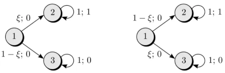
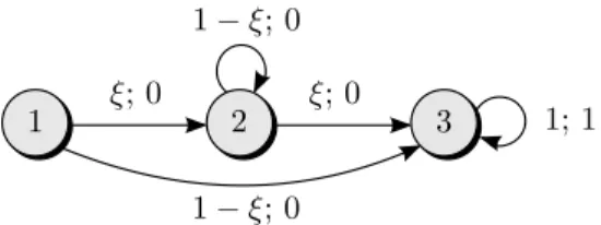
Example 2.2 (Rectangularity) Consider the robust infinite horizon MDP that is shown in Figure 1. The uncertainty set P encompasses all transition kernels that correspond to parameter realisations ξ∈
1 2 ξ 1−ξ 1−ξ ξ 1 2 1−ξ ξ ξ 1−ξ
Figure 1: MDP with two states and two actions. The left and right charts present the transition probabilities for actions 1 and 2, respectively. In both diagrams, nodes correspond to states and arcs to transitions. We label each arc with the probability of the associated transition. We suppressp0 and the expected rewards.
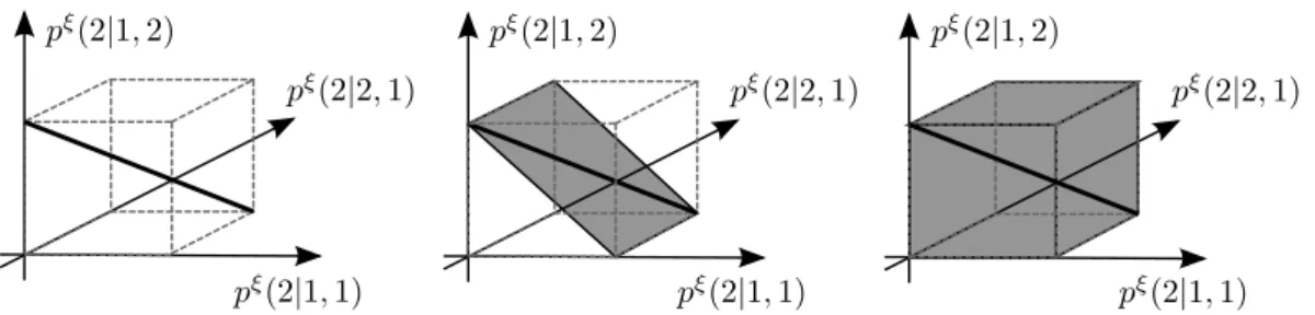
pξ(2 |1,1) pξ(2 |1,1) pξ(2 |1,1) pξ(2 |1,2) pξ(2 |1,2) pξ(2|1,2) pξ(2 |2,1) pξ(2 |2,1) pξ(2 |2,1)
Figure 2: Illustration ofP (left chart) and the smallest s-rectangular (middle chart) and
(s, a)-rectangular (right chart) uncertainty sets that contain P. The charts show three-dimensional projections of P ⊂ R8
. The thick line represents P, while the shaded areas visualise the corresponding rectangular uncertainty sets. Figure 1 implies thatpξ(2|1,1) =ξ,
pξ(2|1,2) = 1−ξandpξ(2|2,1) =ξ. The dashed lines correspond to the unit cube inR3
.
[0,1]. This MDP can be assigned an uncertainty set of the form (3). Figure 2 visualises P and the smallest s-rectangular and(s, a)-rectangular uncertainty sets that contain P.
From now on, we always consider uncertainty sets of the form (3). We may sometimes call a generic uncertainty setnon-rectangular to emphasise that it is neithers- nor (s, a)-rectangular.
2.2
The Robust Policy Improvement Problem
We now consider the policy improvement problem, which asks for a policy that maximises the worst-case expected total reward (2) over an uncertainty set of the form (3). Remember that a policyπrepresents a sequence of functions (πt)t∈T that map state-action histories to probability distributions overA. In
its most general form, such a policy ishistory dependent, that is, at any time period t the policy may assign a different probability distribution to each state-action history (s1, a1, . . . , st−1, at−1;st).
Due to the storage requirements of history dependent policies, one typically prefers more ‘economical’ policy classes. A policyπis calledMarkovian ifπtis determined bystandtfor allt∈ T. A Markovian policy π is called stationary if πt is solely determined by st for all t ∈ T. In finite horizon MDPs, Markovian and stationary policies are equally expressive since the setsStare disjoint. In infinite horizon MDPs, however, stationary policies form a strict subset of the class of Markovian policies. A policy π
is called deterministic if πt places all probability mass on one action for each t ∈ T; otherwise, π is called randomised. In the following, we will focus on stationary policies due to their favourable storage
requirements. We denote by Π the set of all randomised stationary policies for a given MDP instance. It is well-known that non-robust finite and infinite horizon MDPs always allow for a deterministic stationary policy that maximises the expected total reward (1). Optimal policies can be determined via value or policy iteration, or via linear programming. Finding an optimal policy, as well as evaluating (1) for a given stationary policy, can be done in polynomial time. For a detailed discussion, see [4, 19, 22].
To date, the literature on robust MDPs has focused on (s, a)-rectangular uncertainty sets. For this class of uncertainty sets, it is shown in [11, 17] that the worst-case expected total reward (2) is maximised by a deterministic stationary policyπfor finite and infinite horizon MDPs. Optimal policies can be determined via extensions of the value and policy iteration. For some uncertainty sets, finding an optimal policy, as well as evaluating (2) for a given stationary policy, can be achieved in polynomial time. Moreover, the policy improvement problem satisfies the following saddle point condition:
sup π∈Π inf P∈P EP,π "∞ X t=0 λtr(st, at, st+1) s0∼p0 # = inf P∈P sup π∈Π EP,π "∞ X t=0 λtr(st, at, st+1) s0∼p0 # (4)
A similar result for robust finite horizon MDPs is discussed in [17].
We now show that the benign structure of optimal policies over (s, a)-rectangular uncertainty sets partially extends to the broader class ofs-rectangular uncertainty sets.
Proposition 2.3 (s-Rectangular Uncertainty Sets) Consider the policy improvement problem for a finite or infinite horizon MDP over an s-rectangular uncertainty set of the form (3).
(a) There is always an optimal policy that is stationary.
(b) It is possible that all optimal stationary policies are randomised.
Proof As for claim (a), consider a finite horizon MDP with an s-rectangular uncertainty set. By construction, the probabilities associated with transitions emanating from state s∈ S are independent from those emanating from any other states′
∈ S,s′
6
=s. Moreover, each statesis visited at most once since the setsStare disjoint. Hence, any knowledge about past transition probabilities cannot contribute to better decisions in future time periods, which implies that stationary policies are optimal.
Consider now an infinite horizon MDP with an s-rectangular uncertainty set. Appendix A shows that the saddle point condition (4) extends tos-rectangular uncertainty sets. For any fixed transition kernelP∈ P, the supremum over all stationary policies on the right-hand side of (4) is equivalent to the supremum over all history dependent policies. By weak duality, the right-hand side of (4) thus represents an upper bound on the worst-case expected total reward of any history dependent policy. Since there is a stationary policy whose worst-case expected total reward on the left-hand side of (4) attains this upper bound, claim (a) follows.
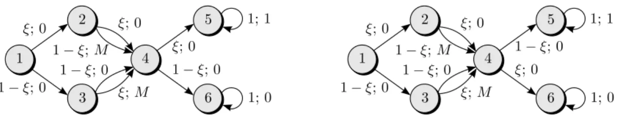
ξ; 0 1−ξ; 0 1; 1 1; 0 1 2 3 1−ξ; 0 ξ; 0 1; 1 1; 0 1 2 3
Figure 3: MDP with three states and two actions. The left and right figures present the transition probabilities and expected rewards for actions1and 2, respectively. The first and second expressions in the arc labels correspond to the probabilities and expected rewards of the associated transitions, respectively. Apart from that, the same drawing conventions as in Figure 1 are used. The initial state distributionp0 places unit mass on state 1.
As for claim (b), consider the robust infinite horizon MDP that is visualised in Figure 3. The uncertainty setP encompasses all transition kernels that correspond to parameter realisationsξ∈[0,1]. This MDP can be assigned an s-rectangular uncertainty set of the form (3). Since the transitions are independent of the chosen actions from time 1 onwards, a policy is completely determined by the decision
β=π0(1|1) at time 0. The worst-case expected total reward is
min ξ∈[0,1] βξ+ (1−β)(1−ξ) λ 1−λ= min{β,1−β} λ 1−λ.
Over β ∈ [0,1], this expression has its unique maximum at β∗ = 1/2, that is, the optimal policy is randomised. If we replace the self-loops with expected terminal rewards ofr2:= 1 andr3:= 0, then we
obtain an example of a robustfinite horizon MDP whose optimal policy is randomised.
Figure 3 illustrates the counterintuitive result that randomisation is superfluous for (s, a)-rectangular uncertainty sets. If we project the uncertainty set P associated with Figure 3 onto its marginalsPsa, then the transition probabilities in the left chart become independent of those in the right chart. In this case, any policy results in an expected total reward of zero, and randomisation becomes ineffective.
We now show that in addition to randomisation, the optimal policy may require history dependence if the uncertainty set lackss-rectangularity.
Proposition 2.4 (General Uncertainty Sets) For finite and infinite horizon MDPs, the policy im-provement problem over non-rectangular uncertainty sets is in general solved by non-Markovian policies.
Proof Consider the robust infinite horizon MDP with six states and two actions that is visualised in Figure 4. The uncertainty set P encompasses all transition kernels that correspond to parameter realisationsξ∈[0,1]. This MDP can be assigned an uncertainty set of the form (3). Since the transitions do not depend on the chosen actions except for π2, a policy is completely determined by the decision
1 2 3 4 5 6 ξ; 0 1−ξ; 0 ξ; 0 1−ξ; M 1−ξ; 0 ξ;M ξ; 0 1−ξ; 0 1; 1 1; 0 1 2 3 4 5 6 ξ; 0 1−ξ; 0 ξ; 0 1−ξ;M 1−ξ; 0 ξ;M 1−ξ; 0 ξ; 0 1; 1 1; 0
Figure 4: MDP with six states and two actions. The initial state distributionp0 places unit
mass on state1. The same drawing conventions as in Figure 3 are used.
The conditional probability to reach state 5 isϕ1(ξ) :=β1ξ+ (1−β1)(1−ξ) if state 2 is visited and
ϕ2(ξ) :=β2ξ+ (1−β2)(1−ξ) if state 3 is visited, respectively. Thus, the expected total reward is
2λξ(1−ξ)M+ λ
3
1−λ[ξ ϕ1(ξ) + (1−ξ)ϕ2(ξ)],
which is concave inξfor allβ∈[0,1]2ifM ≥λ2/(1−λ). Thus, the worst (minimal) expected total reward
is incurred forξ∗∈ {0,1}, independently ofβ∈[0,1]2
. Hence, the worst-case expected total reward is
min ξ∈{0,1} λ3 1−λ[ξ ϕ1(ξ) + (1−ξ)ϕ2(ξ)] = λ3 1−λmin{β1,1−β2},
and the unique maximiser of this expression isβ = (1,0). We conclude that in state 4, the optimal policy chooses action 1 if state 2 has been visited and action 2 otherwise. Hence, the optimal policy is history dependent. If we replace the self-loops with expected terminal rewards ofr5:=λ3/(1−λ) andr6:= 0,
then we can extend the result to robust finite horizon MDPs.
Although the policy improvement problem over non-rectangular uncertainty sets is in general solved by non-Markovian policies, we will restrict ourselves to stationary policies in the remainder. Thus, we will be interested in the best deterministic or randomised stationary policies for robust MDPs.
2.3
Complexity of the Robust Policy Evaluation Problem
We show that the policy evaluation problem over non-rectangular uncertainty sets is stronglyN P-hard. To this end, we will reduce the evaluation of (2) to the 0/1 Integer Programming (IP) problem [8]:
0/1 Integer Programming.
Instance. Given areF ∈Zm×n,g∈Zm, c∈Zn,ζ∈Z.
Question. Is there a vectorx∈ {0,1}n such thatF x≤g andc⊤x
≤ζ?
Assume that x ∈ [0,1]n constitutes a fractional vector that satisfies F x ≤ g and c⊤x
≤ ζ. The following lemma shows that we can obtain an integral vector y ∈ {0,1}n that satisfies F y ≤ g and
c⊤y
≤ζ by roundingxif its components are ‘close enough’ to zero or one.
Lemma 2.5 Let0< ǫ≤min{ǫF, ǫc}, where0< ǫF <minin Pj|Fij|
−1o
and0< ǫc< Pj|cj|
−1
. Assume that x ∈ ([0, ǫ]∪[1−ǫ,1])n satisfies F x ≤ g and c⊤x ≤ ζ. Then F y ≤ g and c⊤y ≤ ζ for
y∈ {0,1}n, whereyj := 1 ifxj ≥1−ǫ andyj := 0otherwise.
Proof By construction,Fi⊤·y≤Fi⊤·x+
P
j|Fij|ǫF < Fi⊤·x+ 1≤gi+ 1 for alli∈ {1, . . . , m}. Similarly, we have thatc⊤y≤c⊤x+Pj|cj|ǫc< c⊤x+ 1≤ζ+ 1. Due to the integrality ofF, g, c, ζ andy, we therefore conclude thatF y≤g andc⊤y
≤ζ.
We can now prove strongN P-hardness of the policy evaluation problem.
Theorem 2.6 Deciding whether the worst-case expected total reward (2) over an uncertainty set of the form (3) exceeds a given valueγ is stronglyN P-hard for deterministic as well as randomised stationary policies and for finite as well as infinite horizon MDPs.
Proof Let us fix an IP instance specified through F, g, c and ζ. W.l.o.g., we can assume that ζ ≤
P
j[cj]
+
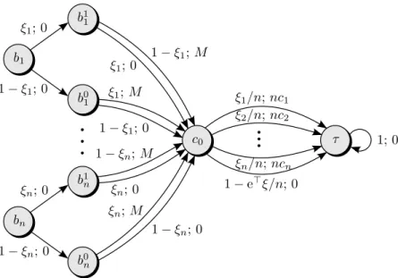
because all feasible IP solutions are binary. We construct a reduction to a robust infinite horizon MDP as follows. The states areS=bj, b1j, bj0 : j= 1, . . . , n ∪ {c0, τ}, there is only one action,
andλ∈(0,1) can be chosen freely. The state transitions and expected rewards are illustrated in Figure 5. The uncertainty setP contains all transition kernels associated withξ∈[0,1]n that satisfyF ξ≤g. We chooseM > λnPj|cj|
/ 2ǫ2, where ǫis chosen as in Lemma 2.5, and set γ :=λ2ζ. Following our
discussion in Section 2.1, the described MDP instance can be constructed in polynomial time with respect to the size of the IP instance (which we henceforth abbreviate as ‘in polynomial time’).1
We show that the answer to the IP instance is affirmative if and only if the worst-case expected total reward (2) does not exceedγ. Indeed, assume that the answer to the IP instance is affirmative, that is, there is a vector x∈ {0,1}n that satisfiesF x≤g and c⊤x
≤ζ. The transition kernel associated with
ξ=xis contained in P and leads to an expected total reward of λ2c⊤ξ
≤λ2ζ =γ. This implies that
the worst-case expected total reward (2) does not exceedγeither. Conversely, assume that (2) does not exceedγ. For the constructed MDP, the expected total reward (1) is continuous inξ. SincePis compact, we can therefore assume that the value of (2) is attained by a transition kernel associated with some
ξ∗
∈Ξ. By construction of Ξ,ξ∗ satisfiesξ∗
∈[0,1]n and F ξ∗
≤g. Assume thatξ∗
q ∈/ ([0, ǫ]∪[1−ǫ,1]) for some q ∈ {1, . . . , n}. In this case, the expected total reward under ξ∗ is greater than or equal to
2λξ∗
q(1−ξq∗)M/n−λ2
P
j[−cj]+ > λ2Pj[cj]+ ≥γ, which contradicts our assumption. We have thus established thatξ∗
∈ ([0, ǫ]∪[1−ǫ,1])n. Under the transition kernel associated with ξ∗, the expected
1
Note that the set Ξ associated with the MDP instance might not contain a Slater point. However, one can decide in polynomial time whether the system of linear equationsF x≤g,x∈[0,1]nis strictly feasible. If this is not the case, one
.
.
.
.
.
.
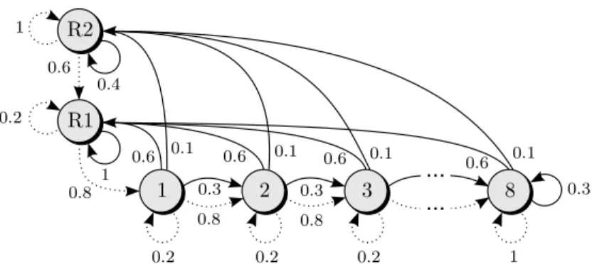
b1 b1 1 b0 1 ξ1; 0 1−ξ1; 0 1−ξ1;M ξ1; 0 ξ1;M 1−ξ1; 0 bn b1 n b0n ξn; 0 1−ξn; 0 1−ξn;M ξn; 0 ξn;M 1−ξn; 0 c0 τ ξ1/n;nc1 ξ2/n;nc2 ξn/n;ncn 1−e⊤ξ/n; 0 1; 0Figure 5: MDP with 3n+ 2states and one action. The distributionp0 places a probability
mass of1/non each statebj,j= 1, . . . , n. The drawing conventions from Figure 3 are used.
reward in periods 0 and 1 is guaranteed to be non-negative, while the expected reward from period 2 onward amounts toλ2c⊤ξ∗. Since the expected total reward underξ∗ does not exceedγ, we therefore
have thatλ2c⊤ξ∗
≤γ=λ2ζ, which implies thatc⊤ξ∗
≤ζ. Hence, we can apply Lemma 2.5 to obtain a vectorξ′
∈ {0,1}n that also satisfiesF ξ′
≤g andc⊤ξ′
≤ζ. We have thus shown that the answer to the IP instance is affirmative if and only if the worst-case expected total reward (2) does not exceedγ.
If we could decide in polynomial time whether the worst-case expected total reward of the constructed MDP exceeds γ, we could also decide IP in polynomial time. Since IP is strongly N P-hard [8], we conclude that the policy evaluation problem (2) is stronglyN P-hard for MDPs with a single action and uncertainty sets of the form (3). Since the policy space of the constructed MDP reduces to a singleton, our proof applies to robust MDPs with deterministic and randomised stationary policies. If we remove the self-loop emanating from stateτ, introduce a terminal reward rτ := 0 and multiply the rewards in
periodtwithλ−t, our proof furthermore applies to robust finite horizon MDPs.
Remark 2.7 Theorem 2.6 remains valid if definition (3) is altered to require thatOl= 0andol∈ {0,1}q. This follows from the fact that IP remains stronglyN P-hard if F andg are binary, see [8].
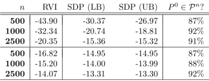
Remark 2.8 Throughout this section we assumed thatP is a convex set of the form (3). If we extend our analysis to nonconvex uncertainty sets, then we obtain the results in Table 1. Note that the complexity of the policy evaluation and improvement problems will be discussed in Sections 2.3, 3 and 4.
uncertainty setP optimal policy complexity (s, a)-rectangular, convex deterministic, stationary polynomial (s, a)-rectangular, nonconvex deterministic, stationary stronglyN P-hard
s-rectangular, convex randomised, stationary polynomial
s-rectangular, nonconvex randomised, history dependent stronglyN P-hard non-rectangular, convex randomised, history dependent stronglyN P-hard
Table 1: Properties of infinite horizon MDPs with different uncertainty sets. From left to right, the columns describe the structure of the uncertainty set, the structure of the optimal policy, and the complexity of the policy evaluation and improvement problems over randomised stationary policies. Each uncertainty set is of the form (3). For nonconvex uncertainty sets, we do not require the matricesOlin (3b) to be negative semidefinite. The properties of finite
horizon MDPs are similar, the only difference being that MDPs withs-rectangular nonconvex uncertainty sets are optimised by randomised stationary policies.
3
Robust Policy Evaluation
It is shown in [11, 17] that the worst-case expected total reward (2) can be calculated in polynomial time for certain types of (s, a)-rectangular uncertainty sets. We extend this result to the broader class of
s-rectangular uncertainty sets in Section 3.1. On the other hand, Theorem 2.6 shows that the evaluation of (2) is strongly N P-hard for non-rectangular uncertainty sets. We therefore develop conservative approximations for the policy evaluation problem over general uncertainty sets in Section 3.2. We bound the optimality gap that is incurred by solving these approximations, and we outline how these approximations can be refined. Although this section primarily sets the stage for the policy improvement problem, we stress that policy evaluation is an important problem in its own right. For example, it finds frequent use in labour economics, industrial organisation and marketing [15].
Our solution approaches fors-rectangular and non-rectangular uncertainty sets rely on the reward to-go function. For a stationary policyπ, we define thereward to-go functionv: Π×Ξ7→RS through
vs(π;ξ) =Ep ξ,π "∞ X t=0 λtr(st, at, st+1) s0=s # fors∈ S. (5)
vs(π;ξ) represents the expected total reward under the transition kernelpξ and the policyπif the initial state iss∈ S. The reward to-go function allows us to express the worst-case expected total reward as
inf ξ∈Ξ Epξ,π "∞ X t=0 λtr(st, at, st+1) s0∼p0 # = inf ξ∈Ξ p⊤0v(π;ξ) . (6)
We simplify our notation by defining the Markov reward process (MRP) induced bypξ andπ. MRPs are Markov chains which pay a state-dependent reward at each time period. In our case, the MRP is given by the transition kernelPb: Π×Ξ7→a RS×Sand the expected state rewards
b
b Pss′(π;ξ) := X a∈A π(a|s)pξ(s′|s, a) (7a) and brs(π;ξ) := X a∈A π(a|s)X s′∈S pξ(s′|s, a)r(s, a, s′). (7b)
Note thatrb(π;ξ)≥0 for eachπ∈Π andξ∈Ξ since all expected rewardsr(s, a, s′) were assumed to be
non-negative. Fors, s′
∈ S,Pbss′(π;ξ) denotes the probability that the next state of the MRP iss′, given
that the MRP is currently in states. Likewise,rbs(π;ξ) denotes the expected reward that is received in states. By taking the expectation with respect to the sample paths of the MRP and reordering terms, we can reformulate the reward to-go function (5) as
v(π;ξ) = ∞ X t=0 h λPb(π;ξ)itrb(π;ξ), (8)
see [19]. The following proposition brings together several results aboutv that we will use later on.
Proposition 3.1 The reward to-go function v has the following properties. (a) v is Lipschitz continuous onΠ×Ξ.
(b) For givenπ∈Πandξ∈Ξ,w∈RS satisfiesw=br(π;ξ) +λPb(π;ξ)w if and only if w=v(π;ξ). (c) For givenπ∈Πandξ∈Ξ, ifw∈RS satisfiesw≤rb(π;ξ) +λPb(π;ξ)w, thenw≤v(π;ξ).
Proof For a square matrix A ∈ Rn×n, let Adj(A) and det(A) denote the adjugate matrix and the determinant ofA, respectively. From equation (8), we see that
v(π;ξ) = I−λPb(π;ξ)−1br(π;ξ) = Adj
I−λPb(π;ξ)br(π;ξ) detI−λPb(π;ξ) ∀
ξ∈Ξ. (9)
Here, the first identity follows from the matrix inversion lemma, see e.g. Theorem C.2 in [19], while the second equality is due to Cramer’s rule. The adjugate matrix and the determinant in (9) constitute polynomials in π and ξ, and the matrix inversion lemma guarantees that the determinant is nonzero throughout Ξ. Hence, the fraction on the right hand-side of (9) has bounded first derivative on Π×Ξ, which implies that it is Lipschitz continuous on Π×Ξ. We have thus proven assertion (A).
Proposition 3.1 allows us to reformulate the worst-case expected total reward (6) as follows. inf ξ∈Ξ p⊤0v(π;ξ) = inf ξ∈Ξ sup w∈RS n p⊤0w : w≤br(π;ξ) +λPb(π;ξ)w o = sup ϑ:Ξ7→RS inf ξ∈Ξ p⊤0ϑ(ξ) : ϑ(ξ)≤br(π;ξ) +λPb(π;ξ)ϑ(ξ) ∀ξ∈Ξ = sup ϑ:Ξ7→cRS inf ξ∈Ξ p⊤0ϑ(ξ) : ϑ(ξ)≤br(π;ξ) +λPb(π;ξ)ϑ(ξ) ∀ξ∈Ξ (10)
Here, the first equality follows from Proposition 3.1 (b)–(c) and non-negativity of p0, while the last
equality follows from Proposition 3.1 (a). Theorem 2.6 implies that (10) is intractable for general uncertainty sets. In the following, we approximate (10) by replacing the space of continuous functions in the outer supremum with the subspaces of constant, affine and piecewise affine functions. Since the policyπis fixed in this section, we may omit the dependence ofv,Pband bronπin the following.
3.1
Robust Policy Evaluation over
s
-Rectangular Uncertainty Sets
We show that the policy evaluation problem (10) is optimised by a constant reward to-go function if the uncertainty setP iss-rectangular. The result also points out an efficient method to solve problem (10).
Theorem 3.2 For an s-rectangular uncertainty setP, the policy evaluation problem (10) is optimised by the constant reward to-go functionϑ∗(ξ) :=w∗,ξ∈Ξ, where w∗∈RS is the unique fixed point of the contraction mappingφ(π;·) :RS 7→RS defined through
φs(π;w) := min ξs∈Ξ n b rs(π;ξs) +λPbs⊤·(π;ξs)w o ∀s∈ S. (11)
Remark 3.3 A functionϕ:RS 7→RS is called contraction mappingif there is someγ∈[0,1)such that
kϕ(w)−ϕ(w′)
k ≤γkw−w′
kfor all w, w′
∈RS. The iterated application ofϕto anyw∈RS converges to the unique fixed pointw∗ that satisfies w∗=ϕ(w∗), see [19].
Proof of Theorem 3.2 We prove the assertion in two steps. We first show thatw∗solves the restriction
of the policy evaluation problem (10) to constant reward to-go functions:
sup w∈RS n p⊤ 0w : w≤rb(ξ) +λPb(ξ)w ∀ξ∈Ξ o (12)
Afterwards, we prove that the optimal values of (10) and (12) coincide fors-rectangular uncertainty sets. In view of the first step, we note that the objective function of (12) is linear inw. Moreover, the feasible region of (12) is closed because it results from the intersection of closed halfspaces parametrised by ξ ∈Ξ. Sincew = 0 is feasible in (12), we can append the constraintw≥ 0 without changing the
optimal value of (12). Hence, the feasible region is also bounded, and we can apply Weierstrass’ extreme value theorem to replace the supremum in (12) with a maximum. Since each of theS one-dimensional inequality constraints in (12) has to be satisfied for allξ∈Ξ, (12) is equivalent to
max w∈RS n p⊤0w : ws≤brs(ξs) +λPbs⊤·(ξs)w ∀s∈ S, ξ1, . . . , ξS ∈Ξ o .
We can reformulate the semi-infinite constraints in this problem to obtain
max w∈RS p⊤0w : ws≤min ξs∈Ξ n b rs(ξs) +λPbs⊤·(ξs)w o ∀s∈ S . (13)
Note that the constraints in (13) are equivalent to w ≤φ(π;w), where φis defined in (11). One can adapt the results in [11, 17] to show that φ(π;·) is a contraction mapping. Hence, the Banach fixed point theorem guarantees existence and uniqueness ofw∗ ∈RS. This vectorw∗ is feasible in (13), and
any feasible solution w ∈ RS to (13) satisfiesw ≤ φ(π;w). According to Theorem 6.2.2 in [19], this
implies that w∗
≥w for every feasible solutionw to (13). By non-negativity of p0, w∗ must therefore
maximise (13). Since (12) and (13) are equivalent, we have thus shown thatw∗ maximises (12).
We now prove that the optimal values of (10) and (13) coincide if P is s-rectangular. Since (13) is maximised by the unique fixed pointw∗of φ(π;
·), we can reexpress (13) as min w∈RS p⊤0w : ws= min ξs∈Ξ n b rs(ξs) +λPbs⊤·(ξs)w o ∀s∈ S .
This problem is equivalent to
min w∈RS ξmins∈Ξ: s∈S n p⊤0w : ws=brs(ξs) +λPbs⊤·(ξs)w ∀s∈ S o . (14)
Thes-rectangularity of the uncertainty setP implies that (14) can be reformulated as
min w∈RS minξ∈Ξ n p⊤0w : ws=brs(ξ) +λPbs⊤·(ξ)w ∀s∈ S o . (15)
For a fixedξ∈Ξ,w=v(ξ) is the unique feasible solution to (15), see Proposition 3.1 (b). By Weierstrass’ extreme value theorem, (15) is therefore equivalent to the policy evaluation problem (10).
The fixed point w∗ of the contraction mapping φ(π;
·) defined in (11) can be found by applying the following robust value iteration. We start with an initial estimate w1 := 0. In the ith iteration,
i= 1,2, . . ., we determine the updated estimatewi+1 viawi+1:=φ(π;wi). Sinceφ(π;
·) is a contraction mapping, the Banach fixed point theorem guarantees that the sequencewiconverges tow∗at a geometric
rate. The following corollary investigates the computational complexity of this approach.
Corollary 3.4 If the uncertainty setP iss-rectangular, then problem (10) can be solved to any accuracy ǫin polynomial time O q3L3/2Slog2
ǫ−1+qAS2logǫ−1.
Proof Assume that at each iterationiof the robust value iteration, we evaluateφ(π;wi) to the accuracy δ:=ǫ(1−λ)2/(4 + 4λ). We stop the algorithm as soon aswN+1
−wN
∞≤ǫ(1−λ)/(1 +λ) at some
iterationN. This is guaranteed to happen withinO logǫ−1iterations [19]. By construction,wN+1 is
feasible for the policy evaluation problem (10), see [19]. We can adapt Theorem 5 from [17] to show that
wN+1satisfies wN+1
−w∗
∞≤ǫ. Hence,w
N+1is also anǫ-optimal solution to (10).
We now investigate the complexity of evaluating φ to the accuracy δ. Under mild assumptions, interior point methods can solve second-order cone programs of the form
min x∈Rn
f⊤x : kAjx+bjk2≤c⊤jx+dj ∀j= 1, . . . , m ,
where Aj ∈Rnj×n, bj ∈Rnj, cj ∈Rn anddj ∈R,j = 1, . . . , m, to any accuracyδin polynomial time
O√mhn3+n2P
jnj
i
logδ−1, see [14]. Forw
∈RS, we can evaluateφ(π;w) by solving the following
second-order cone program:
minimise ξ X a∈A π(a|s) (ksa+Ksaξ)⊤(rsa+λw) (16a) subject to ξ∈Rq Ωl −o⊤ l ξ+ 0 1−ωl 2 2 ≤o⊤l ξ+ ωl+ 1 2 ∀l= 1, . . . , L, (16b)
where (rsa)s′ :=r(s, a, s′) for (s, a, s′)∈ S × A × S and Ωlsatisfies Ω⊤
l Ωl=Ol. We can determine each matrix Ωl in timeO q3
by a Cholesky decomposition, we can construct (16) in timeO qAS+q2L,
and we can solve (16) to accuracyδ in timeO q3L3/2logδ−1. Each step of the robust value iteration
requires the construction and solution of S such problems. Since the constraints of (16) only need to be generated once, this results in an iteration complexity ofO q3L3/2Slogδ−1+qAS2. The assertion
now follows from the fact that the robust value iteration terminates withinO logǫ−1iterations.
Depending on the properties of Ξ defined in (3b), we can evaluate the mapping φmore efficiently. We refer to [11, 17] for a discussion of different numerical schemes.
Remark 3.5 (Finite Horizon MDPs) For a finite horizon MDP, we can solve the policy evaluation problem (10) over ans-rectangular uncertainty setP via robust backward inductionas follows. We start
with wT
∈RS defined through wTs :=rs ifs∈ ST; := 0otherwise. At iteration i=T−1, T −2, . . . ,1,
we determinewi throughwi
s:=φbs(π;wi+1) ifs∈ Si;:=wis+1 otherwise. The operator φbis defined as
b φs(π;w) := min ξs∈Ξ n b rs(π;ξs) +Pbs⊤·(π;ξs)w o ∀s∈ S.
An adaptation of Corollary 3.4 shows that we obtain an ǫ-optimal solution to the policy evaluation problem (10) in timeO q3L3/2Slogǫ−1+qAS2if we evaluateφbto the accuracyǫ/(T
−1).
3.2
Robust Policy Evaluation over Non-Rectangular Uncertainty Sets
If the uncertainty setPis non-rectangular, then Theorem 2.6 implies that constant reward to-go functions are no longer guaranteed to optimise the policy evaluation problem (10). Nevertheless, we can still use the robust value iteration to obtain a lower bound on the optimal value of (10).
Proposition 3.6 Let P be a non-rectangular uncertainty set, and defineP:=
×
s∈SPsas the smallest s-rectangular uncertainty set that containsP. The function ϑ∗(ξ) =w∗ defined in Theorem 3.2 has thefollowing properties.
1. The vector w∗ solves the restriction (12) of the policy evaluation problem (10) that approximates
the reward to-go function by a constant.
2. The functionϑ∗ solves the exact policy evaluation problem (10) overP.
Proof The first property follows from the fact that the first part of the proof of Theorem 3.2 does not depend on the structure of the uncertainty setP. As for the second property, the proof of Theorem 3.2 shows that w∗ minimises (14), irrespective of the structure of
P. The proof also shows that (14) is equivalent to the policy evaluation problem (10) if we replaceP withP.
Proposition 3.6 provides a dual characterisation of the robust value iteration. On one hand, the robust value iteration determines the exact worst-case expected total reward over the rectangularised uncertainty setP. On the other hand, the robust value iteration calculates a lower bound on the worst-case expected total reward over the original uncertainty setP. Hence, rectangularising the uncertainty set is equivalent to replacing the space of continuous reward to-go functions in the policy evaluation problem (10) with the subspace of constant functions.
We obtain a tighter lower bound on the worst-case expected total reward (10) if we replace the space of continuous reward to-go functions with the subspaces of affine or piecewise affine functions. We use the following result to formulate these approximations as tractable optimisation problems.
Proposition 3.7 ForΞ defined in (3b) and any fixedS ∈Sq,s∈Rq andσ∈R, we have ∃γ∈RL+ : σ 1 2s ⊤ 1 2s S − L X l=1 γl ωl 1 2o ⊤ l 1 2ol Ol 0 =⇒ ξ⊤S ξ+s⊤ξ+σ≥0 ∀ξ∈Ξ. (17)
Furthermore, the reversed implication holds if (C1)L= 1or (C2) S0.
Proof Implication (17) and the reversed implication under condition (C1) follow from the approximate and exact versions of theS-Lemma, respectively (see e.g. Proposition 3.4 in [13]).
Assume now that (C2) holds. We define f(ξ) :=ξ⊤S ξ+s⊤ξ+σandg
l(ξ) :=−ξ⊤Olξ−o⊤l ξ−ωl, l= 1, . . . , L. Sincef andg:= (g1, . . . , gL) are convex, Farkas’ Theorem [20] ensures that the system
f(ξ)<0, g(ξ)<0, ξ∈Rq (18a)
has no solution if and only if there is a nonzero vector (κ, γ)∈R+×RL
+ such that
κf(ξ) +γ⊤g(ξ)
≥0 ∀ξ∈Rq. (18b)
Since Ξ contains a Slater pointξ that satisfiesξ⊤Olξ+o⊤l ξ+ω=−gl(ξ)>0,l= 1, . . . , L, convexity of g and continuity off allows us to replace the second strict inequality in (18a) with a less or equal constraint. Hence, (18a) has no solution if and only if f is non-negative on Ξ = {ξ∈Rq : g(ξ)≤0},
that is, if the right-hand side of (17) is satisfied. We now show that (18b) is equivalent to the left-hand side of (17). Assume that there is a nonzero vector (κ, γ)≥0 that satisfies (18b). Note thatκ6= 0 since otherwise, (18b) would not be satisfied by the Slater pointξ. Hence, a suitable scaling of γallows us to setκ:= 1. For our choice off andg, this implies that (18b) is equivalent to
1 ξ ⊤ σ 1 2s⊤ 1 2s S − L X l=1 γl ωl 1 2o⊤l 1 2ol Ol 1 ξ ≥0 ∀ξ∈Rq. (18b’)
Since the above inequality is homogeneous of degree 2 in 1, ξ⊤⊤, it extends to the whole of Rq+1.
Hence, (18b’) is equivalent to the left-hand side of (17).
Proposition 3.7 allows us to bound the worst-case expected total reward (10) from below as follows.
the reward to-go function by an affine function, sup ϑ:Ξ7→aRS inf ξ∈Ξ p⊤0ϑ(ξ) : ϑ(ξ)≤br(ξ) +λPb(ξ)ϑ(ξ) ∀ξ∈Ξ , (19)
as well as the semidefinite program
maximise τ,w,W,γ,Γ τ (20a) subject to τ∈R, w∈RS, W ∈RS×q, γ∈RL +, Γ∈R S×L + p ⊤ 0w−τ 12p⊤0W 1 2W⊤p0 0 − L X l=1 γl ωl 1 2o⊤l 1 2ol Ol 0, (20b) X a∈A π(a|s) k ⊤ sa(rsa+λw) 12 r⊤saKsa+λ k⊤saW+w⊤Ksa 1 2 K ⊤ sarsa+λ W⊤k sa+Ksa⊤w λK⊤ saW − ws 1 2W ⊤ s· 1 2 W ⊤ s· ⊤ 0 − L X l=1 Γsl ωl 1 2o ⊤ l 1 2ol Ol 0 ∀s∈ S, (20c)
where(rsa)s′ :=r(s, a, s′)for (s, a, s′)∈ S × A × S. Let(τ∗, w∗, W∗, γ∗,Γ∗) denote an optimal solution
to (20), and defineϑ∗: Ξ a
7→RS through ϑ∗(ξ) :=w∗+W∗ξ. We have that:
(a) IfL= 1, then (19) and (20) areequivalentin the following sense: τ∗ coincides with the supremum
of (19), andϑ∗ is feasible and optimal in (19).
(b) IfL >1, then (20) constitutes a conservative approximationfor (19): τ∗ provides a lower bound
on the supremum of (19), and ϑ∗ is feasible in (19) and satisfiesinf
ξ∈Ξp⊤0ϑ∗(ξ) =τ∗. Proof The approximate policy evaluation problem (19) can be written as
sup w∈RS, W∈RS×q inf ξ∈Ξ p⊤0 (w+W ξ) : w+W ξ≤br(ξ) +λPb(ξ) (w+W ξ) ∀ξ∈Ξ . (21)
We first show that (21) is solvable. Sincep⊤
0 (w+W ξ) is linear in (w, W) and continuous inξwhile Ξ is
compact, infξ∈Ξp⊤0 (w+W ξ) is a concave and therefore continuous function of (w, W). Likewise, the
feasible region of (21) is closed because it results from the intersection of closed halfspaces parametrised byξ∈Ξ. However, the feasible region of (21) isnot bounded because any non-positive constant reward to-go function, that is, any (w, W) withw∈R− andW = 0, constitutes a feasible solution. However,
since (w, W) = (0,0) is feasible, we can append the constraint w+W ξ ≥ 0 for all ξ ∈ Ξ without changing the optimal value of (21). Moreover, all expected rewards r(s, a, s′) are bounded from above
by r := maxs,a,s′{r(s, a, s′)}. Therefore, Proposition 3.1 (c) implies that any feasible solution (w, W)
for (21) satisfiesw+W ξ≤re/(1−λ) for allξ∈Ξ.
Our results so far imply that any feasible solution (w, W) for (21) satisfies 0≤w+W ξ≤re/(1−λ) for all ξ ∈ Ξ. We now show that this implies boundedness of the feasible region for (w, W). The existence of a Slater point ξ with ξ⊤Olξ+ol⊤ξ+ωl > 0 for all l = 1, . . . , L guarantees that there is an ǫ-neighbourhood of ξ that is contained in Ξ. Hence, W must be bounded because all points ξ in this neighbourhood satisfy 0 ≤w+W ξ ≤ re/(1−λ). As a consequence, w is bounded as well since 0 ≤ w+W ξ ≤ re/(1−λ). Thus, the feasible region of (21) is bounded, and Weierstrass’ extreme value theorem is applicable. Therefore, (21) is solvable. If we furthermore replacePb andrbwith their definitions from (7) and go over to an epigraph formulation, we obtain
maximise τ,w,W τ (22a) subject to τ∈R, w∈RS, W ∈RS×q τ≤p⊤0 (w+W ξ) ∀ξ∈Ξ (22b) ws+Ws⊤·ξ≤ X a∈A π(a|s) (ksa+Ksaξ)⊤(rsa+λ[w+W ξ]) ∀ξ∈Ξ, s∈ S. (22c)
Constraint (22b) is equivalent to constraint (20b) by Proposition 3.7 under condition (C2). Likewise, Proposition 3.7 guarantees that constraint (22c) is implied by constraint (20c). Moreover, if L = 1, condition (C1) of Proposition 3.7 is satisfied, and both constraints are equivalent.
We can employ conic duality [1, 14] to equivalently replace constraint (20b) with conic quadratic constraints. There does not seem to be a conic quadratic reformulation of constraint (20c), however.
Theorem 3.8 provides an exact (forL= 1) or conservative (forL >1) reformulation for the approxi-mate policy evaluation problem (19). Since (19) optimises only over affine approximations of the reward to-go function, Proposition 3.1 (c) implies that (19) provides a conservative approximation for the worst-case expected total reward (10). We will see below that both approximations are tight fors-rectangular uncertainty sets. First, however, we investigate the computational complexity of problem (20).
Corollary 3.9 The semidefinite program (20) can be solved to any accuracy ǫ in polynomial time
O (qS+LS)52(q2S+LS) logǫ−1+q2AS2.
Proof The objective function and constraints of (20) can be constructed in time O q2AS2+q2LS. Under mild assumptions, interior point methods can solve semidefinite programs of the type
min x∈Rn ( c⊤x : F 0+ n X i=1 xiFi 0 ) ,
where Fi ∈ Sm for i = 0, . . . , n, to accuracy ǫ in time O n2m 5
2logǫ−1, see [23]. Moreover, if all matrices Fi possess a block-diagonal structure with blocks Gij ∈Smj, j = 1, . . . , J with Pjmj = m, then the computational effort can be reduced to O n2m1
2P jm2j
. Problem (20) involves O(qS+LS) variables. By exploiting the block-diagonal structure of (20), constraint (20b) gives rise to a single block of dimension (q+ 1)×(q+ 1), constraint set (20c) leads toS blocks of dimension (q+ 1)×(q+ 1) each, and non-negativity ofγ and Γ results inLandSL one-dimensional blocks, respectively.
In Section 4 we discuss a method for constructing uncertainty sets from observation histories. Asymp-totically, this method generates an uncertainty set Ξ that is described by a single quadratic inequality (L= 1), which means that problem (20) can be solved in timeO q92S
7
2logǫ−1+q2AS2. Note that q does not exceedS(S−1)A, the affine dimension of the space [M(S)]S×A, unless some components ofξ
are perfectly correlated. If information about the structure of the transition kernel is available, however,
qcan be much smaller. Section 6 provides an example in whichq remains constant as the problem size (measured in terms ofS, the number of states) increases.
The semidefinite program (20) is based on two approximations. It is a conservative approximation for problem (19), which itself is a restriction of the policy evaluation problem (10) to affine reward to-go functions. We now show that both approximations are tight fors-rectangular uncertainty sets.
Proposition 3.10 Let(τ∗, w∗, W∗, γ∗,Γ∗)denote an optimal solution to the semidefinite program (20),
and define ϑ∗: Ξ7→RS throughϑ∗(ξ) :=w∗+W∗ξ. If the uncertainty setP iss-rectangular, then the
optimal value of the policy evaluation problem (10) isτ∗, andϑ∗ is feasible and optimal in (10).
Proof We show that any constant reward to-go function that is feasible for the policy evaluation prob-lem (10) can be extended to a feasible solution of the semidefinite program (20) with the same objective value. The assertion then follows from the optimality of constant reward to-go functions fors-rectangular uncertainty sets, see Theorem 3.2, and the fact that (20) bounds (10) from below, see Theorem 3.8.
Assume thatϑ: Ξ7→RS withϑ(ξ) =cfor allξ∈Ξ satisfies the constraints of the policy evaluation
problem (10). We show that there is γ ∈ RL+ and Γ∈ R+S×L such that (τ, w, W, γ,Γ) with τ := p⊤0c, w:=candW := 0 satisfies the constraints of the semidefinite program (20). Sinceτ= infξ∈Ξp⊤0ϑ(ξ) ,
ϑin (10) and (τ, w, W, γ,Γ) in (20) clearly attain equal objective values.
By the proof of Theorem 3.8, there is γ ∈ RL+ that satisfies constraint (20b) if and only if τ ≤ p⊤
0 (w+W ξ) for allξ∈Ξ. Sincew+W ξ=c for allξ∈Ξ andτ=p⊤0c, such aγ indeed exists.
Let us now consider constraint set (20c). Since the constant reward to-go functionϑ(ξ) =cis feasible in the policy evaluation problem (10), we have for states∈ S that
1 ξ; 0 2 ξ; 0 3 1−ξ; 0
1−ξ; 0
1; 1
Figure 6: MDP with three states and one action. p0 places unit probability mass on state1.
The same drawing conventions as in Figure 3 are used.
If we replacebrandPbwith their definitions from (7), this is equivalent to
cs≤
X
a∈A
π(a|s)(ksa+Ksaξ)⊤(rsa+λc) ∀ξ∈Ξ,
which is an instance of constraint (22c) wherew=candW = 0. For this choice of (w, W), Proposition 3.7 under condition (C2) is applicable to constraint (22c). Hence, (22c) is satisfied if and only if there is Γ⊤
s·∈R1+×L that satisfies constraint (20c). Since (22c) is satisfied, we conclude that we can indeed find
γand Γ such that (τ, w, W, γ,Γ) satisfies the constraints of the semidefinite program (20).
Propositions 3.6 and 3.10 show that the lower bound provided by the robust value iteration is domi-nated by the bound obtained from the semidefinite program (20). The following example highlights that the quality of these bounds can differ substantially.
Example 3.11 Consider the robust infinite horizon MDP that is visualised in Figure 6. The uncertainty setP encompasses all transition kernels that correspond to parameter realisationsξ∈[0,1]. This MDP can be assigned an uncertainty set of the form (3). Forλ:= 0.9, the worst-case expected total reward is λ2/(1
−λ) = 8.1 and is incurred under the transition kernel corresponding toξ= 1. The solution of the semidefinite program (20) yields the (affine) approximate reward to-go function ϑ∗(ξ) = (6.5,9ξ,10)⊤
and therefore provides a lower bound of 6.5. The unique solution to the fixed point equations w∗ =
φ(w∗), where φ is defined in (11), is w∗ = (0, 0,1/[1−λ]). Hence, the best constant reward to-go
approximation yields a lower bound of zero. Since all expected rewards are non-negative, this is a trivial bound. Intuitively, the poor performance of the constant reward to-go function is due to the fact that it considers separate worst-case parameter realisations for states 1 (ξ= 1) and 2 (ξ= 0).
Example 3.11 shows that the semidefinite program (20) generically provides a strict lower bound on the worst-case expected total reward if the uncertainty set is non-rectangular. In such cases, we would like to estimate the incurred approximation error. Note that we obtain anupper (i.e., optimistic) bound on the worst-case expected total reward if we evaluate p⊤
0v(ξ) for any singleξ ∈ Ξ. Let ϑ∗(ξ)
denote an optimal affine approximation of the reward to-go function obtained from the semidefinite program (20). Thisϑ∗can be used to obtain a suboptimal solution to arg minp⊤
arg minp⊤
0ϑ∗(ξ) : ξ∈Ξ , which is a convex optimisation problem. Let ξ∗ denote an optimal solution
to this problem. We obtain an upper bound on the worst-case expected total reward by evaluating
p⊤0v(ξ∗) = p⊤0 ∞ X t=0 h λPb(ξ∗)itbr(ξ∗) = p⊤0 I−λPb(ξ∗)−1br(ξ∗), (23)
where the last equality follows from the matrix inversion lemma, see e.g. Theorem C.2 in [19]. We can thus estimate the approximation error of the semidefinite program (20) by evaluating the difference between (23) and the optimal value of (20). If this difference is large, the affine approximation of the reward to-go function may be too crude. In this case, one could use modern decision rule techniques [3, 10] to reduce the approximation error via piecewise affine approximations of the reward to-go function. Since the resulting generalisation requires no new ideas, we omit details for the sake of brevity.
Remark 3.12 (Finite Horizon MDPs) Our results can be directly applied to finite horizon MDPs if we convert them to infinite horizon MDPs. To this end, we choose any discounting factorλand multiply the rewards associated with transitions in periodt∈ T byλ−t. Moreover, for every terminal states
∈ ST, we introduce a deterministic transition to an auxiliary absorbing state and assign an action-independent expected reward of λ−Trs. Note that in contrast to non-robust and rectangular MDPs, the approximate policy evaluation problem (20) does not decompose into separate subproblems for each time periodt∈ T.
4
Robust Policy Improvement
In view of (10), we can formulate the policy improvement problem as
sup π∈Π sup ϑ:Ξ7→cRS inf ξ∈Ξ p⊤0ϑ(ξ) : ϑ(ξ)≤br(π;ξ) +λPb(π;ξ)ϑ(ξ) ∀ξ∈Ξ . (24)
Sinceπis no longer fixed in this section, we make the dependence ofv,Pbandbronπexplicit. Section 3 shows that the policy evaluation problem can be solved efficiently if the uncertainty setPiss-rectangular. We now extend this result to the policy improvement problem.
Theorem 4.1 For ans-rectangular uncertainty setP, the policy improvement problem (24) is optimised by the policy π∗
∈ Π and the constant reward to-go function ϑ∗(ξ) := w∗, ξ
∈ Ξ, that are defined as follows. The vectorw∗∈RS is the unique fixed point of the contraction mapping ϕdefined through
ϕs(w) := max
π∈Π{φs(π;w)} ∀s∈ S, (25)
whereφis defined in (11). For eachs∈ S, let πs