A DSATUR-based algorithm for the Equitable Coloring
Problem
✩Isabel M´endez-D´ıaza,1, Graciela Nasinib,c, Daniel Sever´ınb,c a
FCEyN, Universidad de Buenos Aires, Argentina b
FCEIA, Universidad Nacional de Rosario, Argentina c
CONICET, Argentina
Abstract
This paper describes a new exact algorithm for the Equitable Coloring Prob-lem, a coloring problem where the sizes of two arbitrary color classes differ
in at most one unit. Based on the well known DSatur algorithm for the
classic Coloring Problem, a pruning criterion arising from equity constraints is proposed and analyzed. The good performance of the algorithm is shown through computational experiments over random and benchmark instances.
Key words: equitable coloring, DSatur, exact algorithm
2000 MSC: 05C15, 05A15
1. Introduction
There exists a large family of combinatorial optimization problems having relevant practical importance, besides its theoretical interest. One of the most representative problem of this family is the Graph Coloring Problem
(GCP), which arises in many applications such as scheduling, timetabling, electronic bandwidth allocation and sequencing problems.
Given a simple graphG= (V, E), where V is the set of vertices and E is the set of edges, a coloring of G is an assignment of colors to vertices such
✩Partially supported by grants PIP-CONICET 241, PICT 2011-0817 and
UBA-CYT 20020100100666. E-mail addresses: [email protected] (I. M´endez-D´ıaz), [email protected](G. Nasini),[email protected](D. Sever´ın).
1Corresponding author at Departamento de Ciencias de la Computaci´on, Facultad de
Ciencias Exactas y Naturales, Universidad de Buenos Aires, Intendente Guiraldes 2160 (Ciudad Universitaria, Pabell´on 1), Argentina
that the endpoints of any edge have different colors. A k-coloring of G is
a coloring that uses k colors. The GCP consists of finding the minimum
number k such thatGadmits a k-coloring. This minimum number of colors is called the chromatic number of G and is denoted byχ(G).
It is well known that GCP models some scheduling problems. The sim-plest version considers assignments of workers to a given set of tasks. Pairs of tasks may conflict each other, meaning that they should not be assigned to the same worker. The problem is modeled by building a graph containing a vertex for every task and an edge for every conflicting pair of tasks. A col-oring of this graph represents a conflict-free assignment and the chromatic number of the graph is exactly the minimum number of workers needed to perform all tasks.
However, an extra constraint could be required to ensure the uniformity of the distribution of workload employees. The addition of this extra equity
constraint gives rise to the Equitable Coloring Problem (ECP), introduced in [1] and motivated by an application concerning garbage collection [2]. Other applications of the ECP concern load balancing problems in multiprocessor machines [3] and results in probability theory [4]. An introduction to ECP and some basic results are provided in [5].
Formally, an equitable k-coloring (or just k-eqcol) of a graph G is a k -coloring satisfying the equity constraint, i.e. the size of two color classes can
not differ by more than one unit. The equitable chromatic number of G,
χeq(G), is the minimum k for which G admits a k-eqcol. The ECP consists of finding χeq(G).
Computingχeq(G) for arbitrary graphs is proved to be NP-Hard and just a few families of graphs are known to be easy such as complete n-partite, complete split, wheel and tree graphs [5].
There exist some differences between GCP and ECP that make the latter harder to solve. It is known that the chromatic number of an unconnected
graph G is the maximum among the chromatic numbers of its components.
Algorithms that solve GCP can take advantages of the property mentioned above (e.g. [6]) by solving GCP on each component, which is less CPU in-tensive than address the problem on the whole graph. Moreover, one can preprocess the graph in order to reduce its size and, consequently, the time of optimization. For example, choosing two non-adjacent vertices with the same neighborhood, known as twin vertices, and deleting one of them. The chromatic number of the graph remains the same after deletion, since the
deleted vertex can inherit the color of the other one. None of these recipes can be applied when solving ECP. For instance, let G be the graph of Fig-ure 1a and G0
be the graph compounded of two disjoint copies of G. Then,
χeq(G0
) = 2 butχeq(G) = 3. Also, letH0
be the graph of Figure 1b. Clearly,v
andv0
are twin vertices. LetH0
beH afterv is deleted. We haveχeq(H0
) = 2 but χeq(H) = 3.
Figure 1
There are very few tools in the literature related to ECP resolution. Two
constructive algorithms called Naive and SubGraph were given in [5] to
generate greedily an equitable coloring of a graph and, as far as we know, two integer linear programming approaches are available. The first one is a Branch-and-Cut algorithm, called B&C-LF2 [7], which is based on the
asymmetric representatives formulation for GCP described in [8]. The other one [9] adapts to ECP the formulation and techniques used by M´endez-D´ıaz and Zabala for GCP in [6], studies its polyhedral structure and derives families of valid inequalities. Some of them have shown to be very effective as cutting planes in preliminary computational experiments.
Regarding GCP, we can find good exact algorithms which are not based on
IP techniques. One of the most well known example is DSatur, proposed
by Br´elaz in [10]. This Branch-and-Bound algorithm has been referred in the literature several times and is still used by its simplicity, its efficiency in medium-sized graphs and the possibility of applying it at some stage in metaheuristics or in more complex exact algorithms like Branch-and-Cut
ones [6]. Recently, it was shown that a modification of DSatur performs
relatively well compared with many state-of-the-art algorithms based on IP techniques, showing superiority in random instances [11].
in order to address the ECP, which is the goal of this paper. Our approach exploits arithmetical properties inherent in equitable colorings and combines them with the techniques originally developed by Brown [12] and Br´elaz [10] for DSatur, and improved by Sewell [13] and San Segundo [11]. We call it
EqDSatur. A preliminary version of this algorithm with weaker pruning
rules than the one analyzed in this work was already presented in [14]. The paper is organized as follows. Section 2 gives a brief summary of known DSatur-based algorithms for GCP. Section 3 shows the background math for our pruning rule. Section 4 describes an implementation of EqD-Satur. Section 5 discusses methods for obtaining lower and upper bounds of the equitable chromatic number. Section 6 reports computational
exper-iments carried out to tune up the behaviour of EqDSatur, and compares
our algorithm against other ones from the literature. Finally, Section 7 gives final conclusions.
We now introduce some notations and definitions employed throughout the paper. For any positive integer k, [k] denotes the set{1,2, . . . , k}. Given a graph G = (V, E), we assume the set of vertices is V = [n]. A graph for which every vertex is adjacent to each other is called acomplete graph. Given
S ⊂V, we denote by G[S] the subgraph of G induced by S. A set Q⊂V is a clique of Gif G[Q] is a complete graph.
Given u ∈ V, the neighborhood of u is the set of vertices adjacent to
u and is denoted by N(u). The closed neighborhood of u, N[u], is the set
N(u)∪ {u}. Thedegree of u,d(u), is the cardinality of N(u). The maximum degree of vertices in G is denoted by ∆(G).
A stable set is a set of vertices of G no two of which are adjacent. We denote by α(G) thestability number of G, i.e. the maximum cardinality of a stable set of G. Given S ⊂ V, we also denote by α(S) the stability number of G[S].
Apartialk-partitionofG, denoted by Π = (C1, C2, . . . , Cn), is a collection of disjoint sets such that ∪k
j=1Cj ⊂ V and Cj =∅ if and only if j ≥k+ 1.
We write k(Π) to refer the number of non-empty sets in Π. We denote by
U(Π) the set of vertices not covered by the sets of Π, i.e. U(Π) =V\∪k j=1Cj.
If U(Π) = ∅ we say that Π is a k-partition. Given v ∈ V\U, we denote by
Π(v) the number of the set to which v belongs, i.e. v ∈CΠ(v).
A partial k-coloring of Gis a partial k-partition Π = (C1, C2, . . . , Cn) of
G such that each Cj is a stable set of G. In this context, U(Π) is called the
Π is a k-coloring.
Givenv ∈V and a partial k-coloring Π, let DΠ(v) be the set of different colors assigned to the adjacent vertices of v, i.e. DΠ(v) = {Π(w) : w ∈
N(v)\U(Π)}. The saturation degree of v in Π, ρΠ(v), is the cardinality of
DΠ(v) and the set of available colors of v,FΠ(v), is the set of unused colors in the neighborhood of v, i.e. FΠ(v) = [n]\DΠ(v).
Given a partial k-partition Π, u ∈ U(Π) and j ∈ [k + 1] we denote by Π +hu, ji to the partial partition obtained by adding u toCj.
We say that a partial k-partition (or partial k-coloring) Π = (C1, C2,
. . .,Cn)can be extended to a k0
-partition (or k0
-coloring) if there exists ak0
-partition (or k0 -coloring) Π0 = (C0 1, C 0 2, . . . , C 0
n) which can be obtained from Π by succesive applications of the operator “+”. A direct consequence is that k ≤k0
and Cj ⊂Cj0 for all j ∈[k].
We say that a k-partition or k-coloring Π = (C1, C2, . . . , Cn) of G is
equitable if it satisfies the equity constraint, i.e.
||Ci| − |Cj|| ≤1, for i, j ∈[k].
An equitable k-coloring is also called k-eqcol for the sake of simplicity.
2. An overview of DSatur-based algorithms for GCP
The idea behind an enumerative algorithm such asDSatur is to
deter-mine early whether it is possible to extend a partial coloring to a proper coloring so that uncolored vertices are painted with available colors. In this way, the enumerative procedure avoids to explore partial colorings that will not lead to an optimal coloring, and therefore would be needlessly enumer-ated.
DSatur is based on a generic enumerative scheme proposed by Brown
[12], outlined as follows:
Input: Ga graph, Π0 an initial partial coloring of G and Π∗ an initial
col-oring of G.
Output: Π∗ an optimal coloring of G, UB the chromatic number of G.
Algorithm: Set UB ←k(Π∗
Node(Π):
Step 1. If U(Π) =∅, set UB ←k(Π), Π∗ ←Π and return.
Step 2. Select a vertex u∈U(Π).
Step 3. For each color j ∈[min{k(Π) + 1, UB−1}] such that j ∈FΠ(u): Set Π0
←Π +hu, ji.
If FΠ0(v)∩[UB−1]=6 ∅ for all v ∈U(Π0), execute Node(Π0).
The previous scheme only works when the initial partial coloring Π0 can
be extended to an optimal coloring. A suitable Π0 can be computed as
follows: if Q ={v1, v2, . . . , vq} is a maximal clique of G, it is known that a
q-partial coloring Π0 such that Π0(vi) = i for all i ∈ [q] can be extended to
a χ(G)-coloring.
Indeed, we must know a maximal clique Q and an initial coloring Π∗
in advance. Moreover, we must state the rule for choosing vertex u in Step 2 and the order in which colors fromF(u) have to be evaluated. From now on, we call to these criteria vertex selection strategy (VSS) and color selection strategy (CSS).
Br´elaz proposed the algorithm DSatur [10] by obtaining a maximal
clique Qand an initial coloring Π∗
with greedy heuristics (one is SLI given in [15] and the other is contributed by himself). The vertex selection strategy, which we call DSATUR-VSS, selects the uncolored vertex with the largest saturation degree. In case of a tie, select the vertex with the largest degree. More specifically, letρbe the maximum saturation degree of Π and T be the so called set of candidate vertices:
T ={u∈U(Π) :ρΠ(u) =ρ}.
DSATUR-VSS chooses u ∈ T that maximizes d(u). In the case that more
than one vertex inT has the maximum degree, untie them according to some predetermined order, e.g. its number in V.
Sewell [13] suggested a modified tie breaking rule for choosing u from the set T, called Celim (CELIM-VSS). It consists of selecting from the set of vertices tied at maximum saturation degree, the one with the maximum number of common available colors in the neighborhood of uncolored vertices. That is, choose u∈T such that the value
celim(u) = X j∈FΠ(u)
is the highest.
Let us note that, while DSATUR-VSS attempts to estimate future color availability through the degree of vertices, CELIM-VSS also contemplates the impact of coloring a vertex over the uncolored vertices yet. Although CELIM-VSS is more CPU intensive than DSATUR-VSS, fewer nodes are evaluated and, in the case of medium and high density instances, less time is required to reach the optimality.
A further improvement in the vertex selection strategy was recently
pro-posed by San Segundo [11]. The criterion chooses the vertex u ∈ T that
maximizes the value
pass(u) = X j∈FΠ(u)
|{v ∈N(u)∩T :j ∈FΠ(v)}|.
By comparing it with Sewell’s criterion we may observe that CELIM-VSS minimizes the number of subproblems by systematically reducing available color at deeper levels of the search tree. By constrast, San Segundo’s criterion restricts this computation to the neighbors in the set of tied vertices, reducing color domains of vertices which are already known to have the least number of available colors, and so therefore more likely to require a new color at deeper levels of the search tree.
At an early stage of enumeration, the set T has many vertices and the computation of pass(u) induces an overload in the strategy that, in some cases, worsens the overall performance. In order to prevent this overload, a threshold called T H is introduced by the author. If k(Π)−ρ ≤ T H, he chooses from the set T, the vertex u whose value of pass(u) is the highest. Otherwise, he chooses the vertex u whose degree is the highest just like
DSATUR-VSS. This strategy is called Pass (PASS-VSS). Several values of
this threshold were tested in [11] and T H = 3 was settled as the best option. This approach proved to be quite competitive with other exact algorithms for GCP from the literature.
Regarding the color selection strategy, as far as we know, all DSatur-based implementations merely consider the set of available colors in ascending or-der: first evaluate color 1, then color 2, and so on. We call it DSATUR-CSS. Considering the good performance of DSatur-based algorithms for GCP, it is natural to derive an algorithm for ECP consisting of the previous Brown’s
scheme by changing the initial coloring in the initialization by an equitable coloring, and checking whether Π is an equitable coloring in Step 1. In
summary, this simple algorithm, which we call TrivialEqDSatur, only
applies the equity constraint at the leafs of the search tree in the hope that
the resulting coloring is equitable. This may cause TrivialEqDSatur to
explore vast regions of the search tree that will not lead to equitable colorings. Nevertheless, the exploration of useless nodes could be avoided by check-ing, at each node, whether a partial coloring can be extended to an equitable coloring. In the next section, we study necessary and sufficient conditions for a partial coloring to be extended to an equitable coloring and how to implement it as part of a DSatur-based algorithm.
3. A pruning rule for the ECP
We now study arithmetical properties of the sizes of color classes in equi-table colorings and how to combine them in order to propose a pruning rule for our algorithm.
From now on, for a partialk-partition Π = (C1, C2, . . . , Cn), letM(Π) be the largest color class in Π, T(Π) be the index of color classes in Π with size
M(Π), and t(Π) be the cardinality ofT(Π), i.e. M(Π) = max{|Cj|:j ∈[k]},
T(Π) = {j ∈[k] :|Cj|=M(Π)} and t(Π) =|T(Π)|.
The following result fully characterizes when a partial partition can be extended to an equitable partition.
Theorem 1. LetΠbe a partialk-partition, M =M(Π)andt=t(Π). Then,
Π can be extended to an equitable partition if and only if n ≥ M −1
·k+t (1)
Proof. Clearly, if Π can be extended to an equitable partition Π0, then the
classes from T(Π) in Π0
must have at least M vertices. Consequently, the
classes from [k]\T(Π) in Π0
must have at least M −1 vertices. Then, n ≥
M ·t+ (M −1)·(k−t) which is equivalent to (1).
On the other hand, if (1) holds then U(Π) has enough vertices for the following procedure to get an equitable k-partition: add one by one the remaining uncolored vertices to the smallest non-empty class at each step.
Formula (1) allows us to obtain another way of characterizing equitable colorings besides the traditional definition:
Corollary 2. Let Π be a k-coloring of G, M =M(Π) and t =t(Π). Then,
Π is a k-eqcol if and only if (1) holds.
Proof. By Theorem 1, if (1) holds then Π is extended to the equitable k -partition Π itself. Since Π is already a coloring, Π is a k-eqcol. The converse is analogous.
If we wonder when a partial coloring can be extended to an equitable coloring, it is clearly that condition (1) is necessary. However, if we know a lower bound of χeq, the condition can be tightened:
Corollary 3. Let Π be a partial k-coloring, M =M(Π), t =t(Π) and LB be a lower bound of χeq(G). If Π can be extended to an equitable coloring, then
n≥ M−1
·max{k, LB}+t (2)
Proof. In the case that k ≥LB, (2) holds by Theorem 1. Hence, we assume
k < LB. If Π can be extended to an equitable k0
-coloring Π0
, we have that
k0
≥χeq(G)≥LB and classes fromT(Π) in Π0
must have at leastM vertices. Consequently, classes from [LB]\T(Π) in Π0must have at leastM−1 vertices.
Therefore, n≥M ·t+ (M −1)·(LB−t) and (2) holds.
We include the condition given in the previous result as a pruning rule in
the Brown’s scheme. Below, we sketch our approach called EqDSatur:
Input: Ga graph, Π0 an initial partial coloring ofG, Π∗
an initial equitable coloring of Gand LB a lower bound ofχeq(G).
Output: Π∗
an optimal equitable coloring of G, UB =χeq(G).
Algorithm: Set UB ←k(Π∗
). Then, execute Node(Π0).
Node(Π):
Step 1. If U(Π) =∅, set UB ←k(Π), Π∗ ←Π and return.
Step 2. Select a vertex u∈U(Π).
Step 3. For each color j ∈[min{k(Π) + 1, UB−1}] such that j ∈FΠ(u):
Set Π0 ←Π +hu, ji. If n≥ M(Π0 )−1 ·max{k(Π0 ), LB}+t(Π0 ) and
The following theorem shows that EqDSaturworks:
Theorem 4. IfΠ0 can be extended to aχeq(G)-eqcol then EqDSaturgives the value of χeq(G) into the variable UB and an optimal equitable coloring into Π∗
after its execution.
Proof. In the case that (2) does not hold, the node corresponding to Π0
is not called since Π0 can not be extended to an equitable coloring according to
Corollary 3. Therefore, the algorithm does not prune nodes that could reach an optimal equitable coloring.
Also, each coloring reached at Step 1 is indeed an equitable coloring, due to Corollary 2 and the fact that the current coloring satisfies (2).
4. Implementation of EqDSatur
It is clear that the scheme proposed previously is barely helpful if we do not know how to implement it in a efficient way.
Below, we propose a detailed fast implementation of EqDSatur. Inden-tations are meaningful and mark the scope of the operations involved. All sets listed in the implementation are represented by global binary-valued ar-rays. Global variablekis the number of colors of the current partial partition.
Input: G a graph, Π∗ an initial eqcol of Gand LB a lower bound ofχeq(G).
Output: Π∗
an optimal eqcol of G, UB =χeq(G).
Algorithm: Set UB ←k(Π∗
).
Create a partial coloring Π such thatCi ← {vi}for all i∈[q], where
Q={v1, v2, . . . , vq} is a maximal clique of G. Set U(Π)←V\Q and k ←q.
Execute Node(1, q).
Node(M, t):
Step 1. If U(Π) =∅, set UB ←k, Π∗ ←Π and return.
Step 2. Select a vertex u∈U(Π).
Step 3. For eachj ∈[min{k+ 1, UB−1}] such that j ∈FΠ(u): Set size← |Cj|.
If j ≤k, do: If size=M, set t0 ←1 and M0 ←M + 1. If size=M −1, set t0 ←t+ 1 and M0 ←M. If size≤M −2 set t0 ←t and M0 ←M. If j =k+ 1, do: If M = 1, sett0 ←t+ 1 and M0 ←M. If M ≥2, set t0 ←t and M0 ←M. Set previous k←k. Set k ←max{j, k}. If n≥ M0 −1 ·max{k, LB}+t0 , do: Set Cj ←Cj ∪ {u}. Set U(Π)←U(Π)\{u}. Execute Node(M0 , t0 ). Set U(Π)←U(Π)∪ {u}. Set Cj ←Cj\{u}. Set k ←previous k.
We do not describe implemetation details of how to updateFΠ(v) for the
sake of readability, but it can be found in [11]. On the other hand, details of how to compute the clique Q and the initial equitable coloring is discussed in Section 5.
It is not hard to see that variables M and t are indeed the cardinality of the largest class and the number of color classes with size M in the current partial coloring. The update of these variables as well as U(Π), Cj and k is performed in constant time.
UpdatingM and t, and checking (2) is cheap but not free. So, it becames important to analyze if the usage of this pruning rule pays off in terms of CPU time. This task is performed in Section 6 through empirical experimentation.
5. Lower and upper bounds of χeq(G)
In order to initialize EqDSatur, it is necessary to compute bounds of
the equitable chromatic number. In this section, we discuss how to obtain such values and we report some computational experiments related to them. We remark that, in particular, the lower boundLB remains constant during the enumeration, so it is essential that the value of LB be as best as possible.
5.1. Computation of lower bounds
Clearly, every equitable coloring of G is also a classic coloring of G so every lower bound of χ(G) can be used as a lower bound ofχeq(G). In par-ticular, the size of any maximal clique of G is a known lower bound of χ(G) andχeq(G). There are several ways suggested in the literature to obtain such cliques. The easiest method is, for a given graph G and a given vertex v, a greedy algorithm that includes v as the first vertex of the clique and then selects the vertex adjacent to the clique with highest degree in each step until no more vertices can be added to the clique. Furthermore, one may apply this method to different initial vertices v and choose the largest clique. In the case that two cliques of the same size are found, it is advisable to follow a suggestion made by Sewell [13]: retain the clique Qthat maximizes P
q∈Qd(q). The clique found with this criterion will lead to smaller initial sets F(v) since those colors used by the clique will not be available for ver-tices v adjacent to some vertex in the clique. Let us call FindClique(G) to this algorithm.
Let us notice that the distance between χ(G) and χeq(G) can be as far as we want. Such is the case with star graphs K1,m [1] (i.e. a graph K1,m is composed of a vertex v and a stable set S of size m such that v is adjacent to every vertex in S):
χeq(K1,m)−χ(K1,m) = (dm/2e+ 1)−2 =dm/2e −1.
Therefore, it becomes essential to find other lower bounds forχeq(G) besides a maximal clique of G. Lih and Chen [16] proved that
χeq(G)≥
n+ 1
α(V\N[v]) + 2
for anyv ∈V. However, it requires to know the stability number ofG[V\N[v]], an NP-Hard problem [17]. Nevertheless, a relaxation of this value can be used instead. It is known that the cardinality of a partition in cliques of a graph is an upper bound for the stability number of that graph. Let P Cv be the cardinality of a partition in cliques of G[V\N[v]]. The lower the size of the partition is, the tighter the bound becomes. Let us call EqLowBound(G)
to the algorithm that computes the number max n+ 1 P Cv+ 2 :v ∈V ,
where P Cv is obtained by the following greedy heuristic. Initially, let Gv be the graph G[V\N[v]]. We compute a maximal clique of Gv and then we delete those vertices from Gv that belong to the clique found. This simple procedure is repeated until Gv becomes empty, and P Cv is the number of cliques found.
We want to emphasize that both procedures (FindCliqueand
EqLow-Bound) could be improved, thus obtaining better bounds of χeq but at the expense of spending more CPU time.
5.2. Computation of upper bounds
A known upper bound for χeq(G) is ∆(G) + 1 [18], but a slightly better one can be derived from a result stated in [19]: “every graph satisfying
d(u) +d(v) ≤ 2r+ 1 for every edge (u, v), has a (r+ 1)-eqcol”. From this result, it is straightforward to obtain the following relationship:
χeq(G)≤ max{d(u) +d(v) : (u, v)∈E} −1 2 + 1. (3)
Another way for finding an initial upper bound is via heuristics. In our implementation, we adopt Naive[5] which is a heuristic that works well and produces good solutions. Basically, Naive generates a classic coloring with
the algorithm SL [15] and then re-color vertices from the biggest color class to the smallest color class. When it is not possible, a new color is assigned to some vertex from the biggest class. The re-coloring procedure is repeated until an equitable coloring is reached.
5.3. Quality of the bounds
As we said above, it is important to bear in mind the CPU time assigned to the procedures that yield the bounds and how much they will impact in the enumerative algorithm. Since these procedures are fast heuristics, we are not sure whether they yield quality bounds. Next, we analize them through experimentation.
This experiment and all the further ones shown in this paper were carried out on an Intel i5 CPU [email protected] with Ubuntu Linux O.S. and Intel C++ Compiler.
We denote byLBF C to the size of the maximal clique returned by
Find-Clique, LBELB to the lower bound computed by EqLowBound, UB(3) to the upper bound given by (3) and UBN V to the number of colors of the equitable coloring returned by Naive.
Random instances are generated from two parameters: the number of vertices nand the probabilitypthat an edge is included in the graph. Let us note that p is approximately equal to the density of the random graph, i.e.
2|E|
n(n−1).
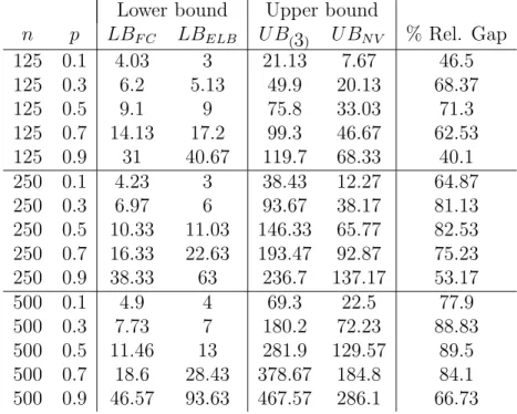
Table 1 summarizes the average of the bounds over 450 ramdomly gen-erated instances of different sizes (each row of the table corresponds to 30 instances). Columns 1-2 show the number of vertices n and probability p of the evaluated instances. Columns 3-6 display the average of LBF C,LBELB,
UB(3) andUBN V, and Column 7 is the average of percentage of relative gap, i.e.
100(min{UBN V, UB(3)} −max{LBF C, LBELB}) min{UBN V, UB(3)}
.
Lower bound Upper bound
n p LBF C LBELB UB(3) UBN V % Rel. Gap
125 0.1 4.03 3 21.13 7.67 46.5 125 0.3 6.2 5.13 49.9 20.13 68.37 125 0.5 9.1 9 75.8 33.03 71.3 125 0.7 14.13 17.2 99.3 46.67 62.53 125 0.9 31 40.67 119.7 68.33 40.1 250 0.1 4.23 3 38.43 12.27 64.87 250 0.3 6.97 6 93.67 38.17 81.13 250 0.5 10.33 11.03 146.33 65.77 82.53 250 0.7 16.33 22.63 193.47 92.87 75.23 250 0.9 38.33 63 236.7 137.17 53.17 500 0.1 4.9 4 69.3 22.5 77.9 500 0.3 7.73 7 180.2 72.23 88.83 500 0.5 11.46 13 281.9 129.57 89.5 500 0.7 18.6 28.43 378.67 184.8 84.1 500 0.9 46.57 93.63 467.57 286.1 66.73
Table 1: Comparison of bounds
As we can see from Table 1, LBELB is particularly useful for medium
(less than a second) can be considered negligible compared to the duration of the enumerative algorithm. Therefore, it is reasonable to have on hand both lower bounds and choose the best one for each case.
Regarding UB(3), it seems to be useless compared to UBN V. Moreover, we did not find any instance such that UBN V ≥UB(3) showing that Naive algorithm is enough to provide good upper bounds.
It is worth mentioning that medium density graphs present the worst average of relative gap. Unfortunately, this issue is transported to the enu-merative algorithm making these instances the hardest to solve.
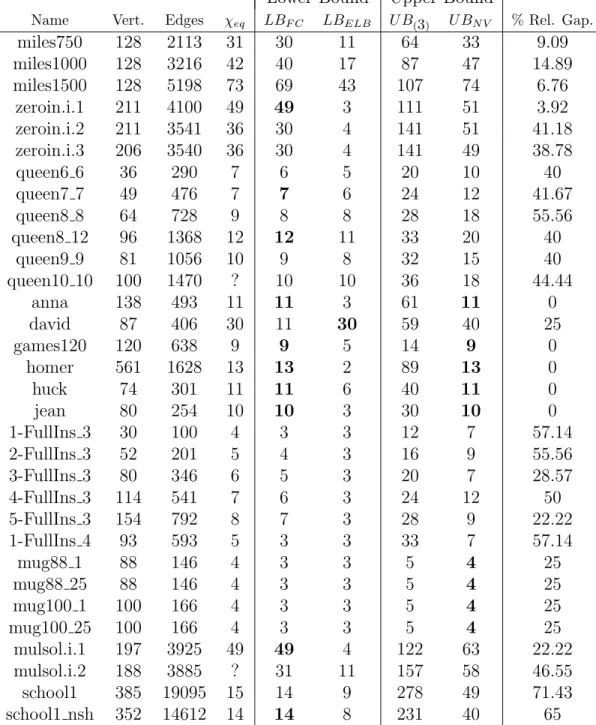
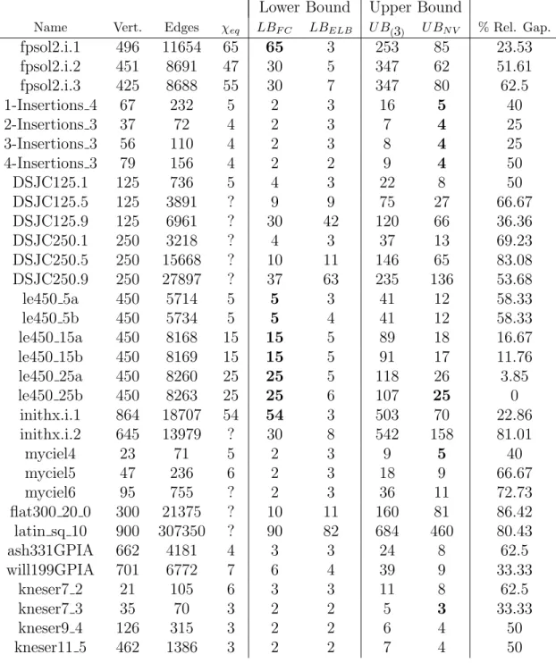
We also evaluated the heuristics on a set of 64 benchmark instances, of which 60 are from a subset of DIMACS COLORLIB library [20] and the re-maining 4 are Kneser graphs [21]. Both COLORLIB and Kneser graphs were already used by other authors for evaluating equitable coloring algorithms (c.f. [7]).
Results are given in Tables 8 and 9. Columns 1-4 show the name of the instance, its number of vertices and edges, and its equitable chromatic number (a question mark “?” meansχeq(G) is unknown so far). Columns 5-9 display the value of the lower bounds, the upper bounds and the percentage of relative gap. Values marked in boldface mean they match with χeq(G).
Similarly to the previous experiment, heuristics took less than one second
for almost all instances. The worst case was latin sq 10 which took 4
seconds.
Let us note that optimality is reached in 6 instances, namely anna,
games120,homer,huck,jeanandle450 25b. Naivealso is able to compute the optimal solution in 10 instances (mug* *, *-Insertions *, myciel4 and kneser7 3). On the other hand,FindCliquereachs the best lower bound in
12 instances (zeroin.i.1, queen7 7,queen8 12,mulsol.i.1,school1 nsh,
fpsol2.i.1,le* * andinithx.i.1) whileEqLowBoundreachs it only for
david.
We conclude that heuristics presented in this section are reasonably fast, simple to implement, and suitable to provide good quality bounds to an exact algorithm.
6. Computational experiments
In this section, we make computational experiments in order to find the best strategies forEqDSaturand compare it against other exact algorithms.
We work with random graphs withn∈ {70,80}andp∈ {0.1,0.3,0.5,0.7,0.9}, and with n= 90 andp∈ {0.1,0.3,0.9}. For each combination ofn andp, we generate T = 30 instances and we analize the performance of our algorithm by considering the following indicators:
• Percentage of solved instances (% solved): An instance is considered “solved” when the time needed to reach the optimal value is at most 2 hours. The percentage of solved instances is the value 100.|S|/T where
S is the set of solved instances.
• Average of the best upper bound reached (Av. UB): It is the average of the upper bound obtained after the enumeration, over all T instances.
• Average of nodes evaluated (Av. Nodes): It is the average of nodes evaluated of the search tree over the set of solved instances S.
• Average of time elapsed (Av. Time): It is the average of time in seconds needed to solve each instance, over the set of solved instances S. We report them on tables, where each row corresponds to a different combi-nation of nand p, and each column displays the value of an indicator for the strategy to be compared. In general, best values are marked in boldface. We do not evaluate combinations n = 90 with p∈ {0.5,0.7} since DSatur-based algorithms (including ours) solves few instances in those cases and compar-isons become rough. The total number of instances amounts to 390.
When we compare two strategies A and B, it may happen that the
in-stances solved by A and B are different and the comparison of the averages of nodes and time may be ambiguous or unfair. In those cases, we consider these averages over the set of instances solved by both strategies: if SA and
SB are the set of solved instances forAand B respectively, we also compute the average of nodes and time over the setSA∩SB. These values are reported with a mark “†”.
6.1. Vertex selection strategy
The following experiment compares an implementation of EqDSatur
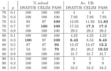
with the three vertex selection strategies mentioned in Section 2 namely DSATUR-VSS, CELIM-VSS and PASS-VSS. Tables 2-3 resume the results. As we can see, PASS-VSS has been able to solve more instances than the other strategies. Also, PASS-VSS performs better in terms of time.
% solved Av. UB
n p DSATUR CELIM PASS DSATUR CELIM PASS
70 0.1 100 100 100 4 4 4 70 0.3 100 100 100 7.93 7.93 7.93 70 0.5 93 97 100 12.03 11.93 11.83 70 0.7 97 100 100 17.53 17.3 17.3 70 0.9 100 100 100 29.2 29.2 29.2 80 0.1 100 100 100 4.23 4.23 4.23 80 0.3 100 97 100 8.43 8.53 8.43 80 0.5 87 87 93 13.47 13.47 13.2 80 0.7 53 50 70 20.1 20.2 19.53 80 0.9 100 100 100 31.7 31.7 31.7 90 0.1 100 100 100 5 5 5 90 0.3 100 100 100 9 9 9 90 0.9 100 100 100 34.2 34.2 34.2
Table 2: Tests on different vertex selection strategies
Av. Nodes Av. Time
n p DSATUR CELIM PASS DSATUR CELIM PASS
70 0.1 216 168 208 0 0 0 70 0.3 401862 253181 171448 0.1 0.1 0.07 70 0.5 6116237 5134138 4702843 6.61 7.76 6.7 70 0.7 21048794 11175213 12020710 28.2 23.5 21 70 0.9 249682 145481 138057 0.17 0.17 0.1 80 0.1 1132 967 5186 0 0 0 80 0.3 31102992 17153530 15495305 27.7 25.2 22.7 80 0.5 540416906 333631281 192172556 601 574 324 80 0.7 821110267 480890653 959670395 1263 1162 1817 675165908† 308409086† 410011950† 1035† 749† 791† 80 0.9 5513947 3098276 3817790 8.2 7.6 6.57 90 0.1 4521 3186 2875 0 0 0 90 0.3 83857234 58179096 32510740 86.8 88.6 52 90 0.9 144093673 71388770 73185398 305 218 161
Table 3: Tests on different vertex selection strategies
Nevertheless, DSATUR-VSS and CELIM-VSS reports less time than PASS-VSS for graphs of 80 vertices and p= 0.7. Since PASS-VSS has solved more instances than the other two strategies, we have added an extra row marked with “†” reporting averages for the three strategies over the instances that
the three strategies have been able to solve simultaneously. Here, CELIM-VSS seems to be a little better than PASS-CELIM-VSS. In our opinion, it is not worth considering these small improvements at the expense of solving fewer instances.
Our conclusion is that PASS-VSS is the right choice for our algorithm.
6.2. Color selection strategy
We contemplate four options:
• DSATUR-CSS. Consider the set of available colors in ascending order.
• BCCOL-CSS [6]. First consider the new color (k+ 1) and then the set of available colors in ascending order.
• ORDER1-CSS. Sort color classes of Π according to their size in as-cending order: |Ci1| ≤ |Ci2| ≤ . . .≤ |Cik|. Then consider colors in the
following order: i1, i2, . . ., ik,k+ 1.
• ORDER2-CSS. Do the same as in ORDER1-CSS but considering colors in the following order: k+ 1, i1,i2,. . .,ik.
BCCOL-CSS is implemented as part of the branching strategy in the Branch-and-Cut BC-Col and the idea is that it tends to find feasible col-orings quickly, albeit not good since it introduces new colors to reach them. ORDER1-CSS is inspired in the heuristic presented in [22]. This rule tends to balance the sizes of color classes and finds equitable colorings early. The downside is that a QuickSort must be performed on each node. ORDER2-CSS is a mix between ORDER1-ORDER2-CSS and BCCOL-ORDER2-CSS. Since we have noticed that it does not perform as well as the others, we do not report it.
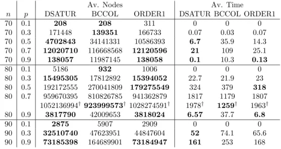
Results for DSATUR-CSS, BCCOL-CSS and ORDER1-CSS are resumed in Tables 4-5.
We first analyze the differences between the classical strategy
DSATUR-CSS and BCCOL-DSATUR-CSS, where the latter performs quite well for n = 80
and p = 0.7. We have noticed that both strategies do not solve the same instances, hence the discrepancy between solved instances (70% and 73% respectively) and average of UB (19.5 and 20.3 respectively), so we have added an extra row reporting averages over the instances that both strategies have been able to solve simultaneously. Although, by inspecting the extra
% solved Av. UB
n p DSATUR BCCOL ORDER1 DSATUR BCCOL ORDER1
70 0.1 100 100 100 4 4 4 70 0.3 100 100 100 7.93 7.93 7.93 70 0.5 100 100 100 11.8 11.8 11.8 70 0.7 100 93 100 17.3 17.8 17.3 70 0.9 100 77 100 29.2 30.8 29.2 80 0.1 100 100 100 4.23 4.23 4.23 80 0.3 100 93 100 8.43 8.63 8.43 80 0.5 93 93 93 13.2 13.3 13.2 80 0.7 70 73 70 19.5 20.3 19.5 80 0.9 100 90 100 31.7 32.5 31.7 90 0.1 100 100 100 5 5 5 90 0.3 100 100 100 9 9 9 90 0.9 100 80 100 34.2 36.5 34.2
Table 4: Tests on different color section strategies
Av. Nodes Av. Time
n p DSATUR BCCOL ORDER1 DSATUR BCCOL ORDER1
70 0.1 208 208 311 0 0 0 70 0.3 171448 139351 166733 0.07 0.03 0.07 70 0.5 4702843 34141331 10586393 6.7 35.9 14.3 70 0.7 12020710 116668568 12120596 21 109 25.1 70 0.9 138057 11987145 138058 0.1 10.3 0.13 80 0.1 5186 932 1006 0 0 0 80 0.3 15495305 17812892 15394052 22.7 21.9 23 80 0.5 192172555 270041809 179275549 324 379 318 80 0.7 959670395 810826785 941362879 1817 1179 1807 1052136994† 923999573† 1028274591† 1978† 1259† 1963† 80 0.9 3817790 42009653 3818024 6.57 37.7 6.8 90 0.1 2875 5907 2909 0 0 0 90 0.3 32510740 47623951 44847604 52 74.1 65.6 90 0.9 73185398 164689901 73184947 161 253 168
Table 5: Tests on different color section strategies
row, BCCOL-CSS solves the “common” instances 57% faster than DSATUR-CSS, the performance of BCCOL-CSS is worse for most of the remaining rows.
Regarding ORDER1-CSS, we can note that there are few differences be-tween this strategy and DSATUR-CSS. Both strategies solves the same in-stances and reaches the same UB for every non-solved graph. The time used by DSATUR-CSS is slightly less than ORDER1-CSS for graphs of 70 and 90 vertices. For n = 80 and p ∈ {30,50}, ORDER1-CSS evaluates 7% and 2% less nodes respectively than DSATUR-CSS. Since ORDER1-CSS performs a QuickSort at each node, the differences in time among these strategies fall to 2% and 0.6% respectively.
We choose DSATUR-CSS for our implementation of EqDSatur, but
ORDER1-CSS may be considered as an alternative strategy anywise.
6.3. TrivialEqDSatur vs. EqDSatur
Our next experiment consists of comparing TrivialEqDSatur and
EqDSatur implementations in order to verify whether the pruning rule
given in Section 3 is efficient. We recall thatTrivialEqDSatur is a simple modification of the standard DSatur that checks whether the colorings at the leafs of the search tree are equitable or not. Both algorithms use the same selection strategies previously chosen and the same bounds given by
the heuristics proposed in Section 5 (althoughTrivialEqDSatur does not
take advantage of the value of LB). Table 6 resumes the results.
% solved Av. UB Av. Nodes Av. Time
n p Triv. EqDS Triv. EqDS Triv. EqDS Triv. EqDS
70 0.1 100 100 4 4 264721 208 0 0 70 0.3 100 100 7.93 7.93 168862113 171448 32.7 0.07 70 0.5 100 100 11.8 11.8 88287477 4702843 29.9 6.7 70 0.7 100 100 17.3 17.3 37918448 12020710 29 21 70 0.9 100 100 29.2 29.2 2776802 138057 1.07 0.1 80 0.1 100 100 4.23 4.23 130316183 5186 20.6 0 80 0.3 100 100 8.43 8.43 345842251 15495305 99.6 22.7 80 0.5 83 93 13.6 13.2 1614284274 192172556 705 324 80 0.7 67 70 19.6 19.5 897961603 959670395 1665 1817 897961603† 828204878† 1665† 1585† 80 0.9 100 100 31.7 31.7 122216644 3817790 54 6.57 90 0.1 100 100 5 5 15428656 2875 2.47 0 90 0.3 100 100 9 9 124572212 32510740 75.9 52 90 0.9 100 100 34.2 34.2 75124470 73185398 169 161
We have noticed that every instance solved by TrivialEqDSatur has been solved by EqDSaturtoo, but not conversely. This fact led us to insert
an extra row in the table for the case n = 80 and p= 0.7, where we report
the average of nodes evaluated and time elapsed of EqDSatur for those
instances that have been solved by TrivialEqDSatur.
We can observe that EqDSatur outperforms TrivialEqDSatur for
all the indicators.
6.4. Comparing against other exact algorithms
This subsection is devoted to compare EqDSatur against the
Branch-and-Cut B&C-LF2 described in [7] and the general purpose solver CPLEX 12.4 with the IP formulation given in [9] and the initial bounds computed by the heuristics given in Section 5.
In the first experiment, we consider 30 instances for each combination of n ∈ {60,70} and p ∈ {0.1,0.3,0.5,0.7,0.9}. We also consider n ∈ {80,100,120} with p = 0.1 and n = 80 with p = 0.9 since CPLEX solves
very few medium-density random instances with n ≥80. The total number
of instances amounts to 420.
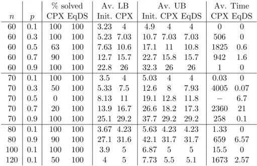
Table 7 summarizes the results, where LB and UB are averaged over
all instances while the time elapsed is averaged over solved instances. A mark “−” is reported when no instance is solved. Columns called “Init.” correspond to the bounds computed by the initial heuristics.
We note that our algorithm is able to solve more instances than CPLEX in considerably less time. The differences are more pronounced in medium density instances.
We do not compare EqDSatur directly against B&C-LF2 since values
reported in [7] consider different random instances. Despite this, we remark that B&C-LF2 has failed to solve any instance withn= 70 andp∈ {0.3,0.5}
whereas EqDSaturcan solve instances of the same size without difficulty.
The last experiment consists of comparing EqDSatur against CPLEX
and B&C-LF2 on DIMACS COLORLIB instances and Kneser graphs
pro-posed in Section 5, except those instances that have been already solved by the initial heuristics. Besides DSATUR-CSS, we also take into account the alternative color strategy ORDER1-CSS.
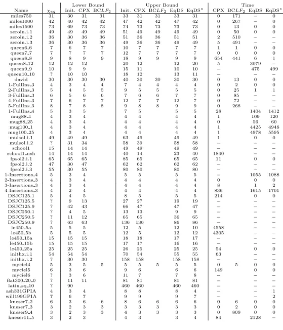
Table 10 reports the final results. Columns 1-2 display the name of the instance and its equitable chromatic number. Columns 3-5 and 6-10 show the bounds given by the initial heuristics and the bounds obtained by each
% solved Av. LB Av. UB Av. Time n p CPX EqDS Init. CPX Init. CPX EqDS CPX EqDS 60 0.1 100 100 3.23 4 4.9 4 4 0 0 60 0.3 100 100 5.23 7.03 10.7 7.03 7.03 506 0 60 0.5 63 100 7.63 10.6 17.1 11 10.8 1825 0.6 60 0.7 90 100 12.7 15.7 22.7 15.8 15.7 942 1.6 60 0.9 100 100 22.8 26 32.3 26 26 1 0 70 0.1 100 100 3.5 4 5.03 4 4 0.03 0 70 0.3 50 100 5.33 7.5 12.6 8 7.93 4005 0.07 70 0.5 0 100 8.13 11 19.1 12.8 11.8 − 6.7 70 0.7 20 100 13.9 16.7 26.6 18.2 17.3 2360 21 70 0.9 100 100 25.1 29.2 37.7 29.2 29.2 258 0.1 80 0.1 100 100 3.67 4.23 5.63 4.23 4.23 1.33 0 80 0.9 90 100 27.1 31.6 42.1 31.7 31.7 659 6.57 100 0.1 100 100 3.9 5 6.87 5 5 15.5 0 120 0.1 50 100 4 5 7.73 5.5 5.1 1673 2.57
Table 7: Performance of EqDSaturand CPLEX on random graphs
algorithm after its execution. Finally, columns 11-14 show the time needed to solve the instance, or “−” if the algorithm is not able to solve it within the limit of two hours. Columns called “EqDS” and “EqDS∗” correspond to
EqDSatur with DSATUR-CSS and ORDER1-CSS respectively.
Results for B&C-LF2 are taken from [7]. We leave blank when the in-stance is not mentioned in that paper. We also recall that these results had been obtained with a slightly different platform: an 1.8 GHz AMD-Atlon machine with Linux and XPRESS 2005-a as the linear programming solver.
From the 58 evaluated instances, CPLEX has solved 38,EqDSaturwith
DSATUR-CSS has solved 29 and with ORDER1-CSS has solved 31. How-ever, some of the instances not solved by both versions of EqDSatur(more
precisely, 3-FullIns 3, 4-FullIns 3 and 5-FullIns 3) are indeed hard to solve by enumerative schemes, as reported in [11], so in our opinion EqD-Satur presents the expected behaviour. On the other hand, both versions
of EqDSaturoutperform CPLEX and B&C-LF2 inqueen8 8, and CPLEX
in myciel5 and queen9 9. In particular, the version with ORDER1-CSS
outperforms B&C-LF2 inmiles750 and miles1000.
ORDER1-CSS for the set of instances solved by both. Also, it is able to solvequeen8 12
andkneser11 5in more than half an hour. Nevertheless, by using
ORDER1-CSS, miles750, miles1000, ash331GPIA and will199GPIA can be solved
without difficulty.
7. Conclusions
In this paper, we present and analyze an exact DSatur-based algorithm for ECP. We propose a pruning rule based on arithmetical properties related to equitable partitions, which has shown to be very effective. We also discuss several color and vertex selection strategies and how to obtain lower and up-per bounds of the equitable chromatic number for initializing the algorithm. Finally, several experiments were carried out to conclude that our approach can tackle the resolution of random graphs better than other algorithms found in the literature so far.
References
[1] Meyer W. Equitable Coloring. Amer. Math. Monthly 1973;80:920–2. [2] Tucker A. Perfect graphs and an application to optimizing municipal
services. SIAM Review 1973;15:585–90.
[3] Das SK, Finocchi I, Petreschi R. Conflict-free star-access in parallel memory systems. J. Parallel Distrib. Comput. 2006;66:1431–41.
[4] Pemmaraju SV. Equitable colorings extend Chernoff-Hoeffding bounds. Approximation, Randomization, and Combinatorial Optimization: Al-gorithms and Techniques, Lecture Notes in Comput. Sci. 2001;2129:285– 96.
[5] Furmanczyk H, Kubale M. Equitable coloring of graphs. In: Graph Colorings, Providence, Rhode Island: American Mathematical Society; 2004, p. 35–53.
[6] M´endez-D´ıaz I, Zabala P. A branch-and-cut algorithm for graph color-ing. Discrete Appl. Math. 2006;154:826–47.
[7] Bahiense L, Frota Y, Noronha TF, Ribeiro C. A branch-and-cut algo-rithm for the equitable coloring problem using a formulation by repre-sentatives. Discrete Appl. Math. 2014;164:34–46.
[8] Campˆelo M, Corrˆea R, Campos V. On the asymmetric representa-tives formulation for the vertex coloring problem. Discrete Appl. Math. 2008;156:1097–111.
[9] M´endez D´ıaz I, Nasini G, Sever´ın D. A polyhedral approach for the Equitable Coloring Problem. Discrete Appl. Math. 2014;164:413–26. [10] Br´elaz D. New methods to color the vertices of a graph. Comm. of the
ACM 1979;22:251–6.
[11] San Segundo P. A new DSATUR-based algorithm for exact vertex col-oring. Comput. Oper. Res. 2012;39:1724–33.
[12] Brown JR. Chromatic scheduling and the chromatic number problem. Manag. Sci (Part I) 1972;19:456–63.
[13] Sewell EC. An improved algorithm for exact graph coloring. In: Trick MA, Johnson DS, editors. Cliques, coloring and satisfiability. Proceed-ings of the second DIMACS implementation challenge, vol. 26. American Mathematical Society; 1996, p. 359–73.
[14] M´endez D´ıaz I, Nasini G, Sever´ın D. An exact DSatur-based algorithm for the Equitable Coloring Problem. Electron. Notes Discrete Math. 2013;44:281–6.
[15] Isaacson JD, Marble G, Matula DW. Graph coloring algorithms. In: Graph Theory and Computing, New York: Academic Press; 1972, p. 109–22.
[16] Lih K-W, Chen B-L. Equitable coloring of trees. J. Combin. Theory, Series B 1994;61:83–7.
[17] Garey. M, Johnson D. Computers and intractability: a guide to the theory of NP completeness. San Francisco, California: Freeman; 1979. [18] Hajnal A, Szemer´edi E. Proof of a conjecture of P. Erd¨os. Combin.
theory and its app. 1970;2:601–23.
[19] Kierstead HA, Kostochka AV. An ore-type theorem on equitable color-ing. J. Combin. Theory Ser. B 2008;98:226–34.
[21] Chen B-L, Huang K-C. The equitable colorings of Kneser graphs. Tai-wanese Journal of Mathematics 2008;12:887–900.
[22] Br´elaz D, Nicolier Y, de Werra D. Compactness and balancing in scheduling. Math. Methods Oper. Res. 1977;21:65–73.
Lower Bound Upper Bound
Name Vert. Edges χeq LBF C LBELB U B(3) U BN V % Rel. Gap.
miles750 128 2113 31 30 11 64 33 9.09 miles1000 128 3216 42 40 17 87 47 14.89 miles1500 128 5198 73 69 43 107 74 6.76 zeroin.i.1 211 4100 49 49 3 111 51 3.92 zeroin.i.2 211 3541 36 30 4 141 51 41.18 zeroin.i.3 206 3540 36 30 4 141 49 38.78 queen6 6 36 290 7 6 5 20 10 40 queen7 7 49 476 7 7 6 24 12 41.67 queen8 8 64 728 9 8 8 28 18 55.56 queen8 12 96 1368 12 12 11 33 20 40 queen9 9 81 1056 10 9 8 32 15 40 queen10 10 100 1470 ? 10 10 36 18 44.44 anna 138 493 11 11 3 61 11 0 david 87 406 30 11 30 59 40 25 games120 120 638 9 9 5 14 9 0 homer 561 1628 13 13 2 89 13 0 huck 74 301 11 11 6 40 11 0 jean 80 254 10 10 3 30 10 0 1-FullIns 3 30 100 4 3 3 12 7 57.14 2-FullIns 3 52 201 5 4 3 16 9 55.56 3-FullIns 3 80 346 6 5 3 20 7 28.57 4-FullIns 3 114 541 7 6 3 24 12 50 5-FullIns 3 154 792 8 7 3 28 9 22.22 1-FullIns 4 93 593 5 3 3 33 7 57.14 mug88 1 88 146 4 3 3 5 4 25 mug88 25 88 146 4 3 3 5 4 25 mug100 1 100 166 4 3 3 5 4 25 mug100 25 100 166 4 3 3 5 4 25 mulsol.i.1 197 3925 49 49 4 122 63 22.22 mulsol.i.2 188 3885 ? 31 11 157 58 46.55 school1 385 19095 15 14 9 278 49 71.43 school1 nsh 352 14612 14 14 8 231 40 65
Lower Bound Upper Bound
Name Vert. Edges χeq LBF C LBELB U B(3) U BN V % Rel. Gap.
fpsol2.i.1 496 11654 65 65 3 253 85 23.53 fpsol2.i.2 451 8691 47 30 5 347 62 51.61 fpsol2.i.3 425 8688 55 30 7 347 80 62.5 1-Insertions 4 67 232 5 2 3 16 5 40 2-Insertions 3 37 72 4 2 3 7 4 25 3-Insertions 3 56 110 4 2 3 8 4 25 4-Insertions 3 79 156 4 2 2 9 4 50 DSJC125.1 125 736 5 4 3 22 8 50 DSJC125.5 125 3891 ? 9 9 75 27 66.67 DSJC125.9 125 6961 ? 30 42 120 66 36.36 DSJC250.1 250 3218 ? 4 3 37 13 69.23 DSJC250.5 250 15668 ? 10 11 146 65 83.08 DSJC250.9 250 27897 ? 37 63 235 136 53.68 le450 5a 450 5714 5 5 3 41 12 58.33 le450 5b 450 5734 5 5 4 41 12 58.33 le450 15a 450 8168 15 15 5 89 18 16.67 le450 15b 450 8169 15 15 5 91 17 11.76 le450 25a 450 8260 25 25 5 118 26 3.85 le450 25b 450 8263 25 25 6 107 25 0 inithx.i.1 864 18707 54 54 3 503 70 22.86 inithx.i.2 645 13979 ? 30 8 542 158 81.01 myciel4 23 71 5 2 3 9 5 40 myciel5 47 236 6 2 3 18 9 66.67 myciel6 95 755 ? 2 3 36 11 72.73 flat300 20 0 300 21375 ? 10 11 160 81 86.42 latin sq 10 900 307350 ? 90 82 684 460 80.43 ash331GPIA 662 4181 4 3 3 24 8 62.5 will199GPIA 701 6772 7 6 4 39 9 33.33 kneser7 2 21 105 6 3 3 11 8 62.5 kneser7 3 35 70 3 2 2 5 3 33.33 kneser9 4 126 315 3 2 2 6 4 50 kneser11 5 462 1386 3 2 2 7 4 50
Lower Bound Upper Bound Time
Name χeq Init. CPX BCLF2 Init. CPX BCLF2 EqDS EqDS∗ CPX BCLF2 EqDS EqDS∗
miles750 31 30 31 31 33 31 31 33 31 0 171 − 0 miles1000 42 40 42 42 47 42 42 47 42 0 267 − 0 miles1500 73 69 73 73 74 73 73 73 73 0 13 0 0 zeroin.i.1 49 49 49 49 51 49 49 49 49 0 50 0 0 zeroin.i.2 36 30 36 36 51 36 36 51 51 2 510 − − zeroin.i.3 36 30 36 36 49 36 36 49 49 5 491 − − queen6 6 7 6 7 7 10 7 7 7 7 1 1 0 0 queen7 7 7 7 7 7 12 7 7 7 7 0 0 0 0 queen8 8 9 8 9 9 18 9 9 9 9 654 441 6 1 queen8 12 12 12 12 20 12 12 20 5 3079 − queen9 9 10 9 9 15 11 10 10 − 475 499 queen10 10 ? 10 10 18 12 13 11 − − − david 30 30 30 30 40 30 30 30 30 0 13 0 0 1-FullIns 3 4 3 4 4 7 4 4 4 4 0 2 0 0 2-FullIns 3 5 4 5 5 9 5 5 5 5 0 25 1 1 3-FullIns 3 6 5 6 6 7 6 6 7 7 0 85 − − 4-FullIns 3 7 6 7 7 12 7 7 12 7 0 72 − − 5-FullIns 3 8 7 8 8 9 8 8 9 9 0 268 − − 1-FullIns 4 5 3 5 7 5 5 5 28 1404 1412 mug88 1 4 3 4 4 4 4 4 1 109 120 mug88 25 4 3 4 4 4 4 4 0 56 60 mug100 1 4 3 4 4 4 4 4 1 4425 4946 mug100 25 4 3 4 4 4 4 4 1 4978 5595 mulsol.i.1 49 49 49 63 49 49 49 1 0 0 mulsol.i.2 ? 31 34 58 39 58 58 − − − school1 15 14 14 49 49 49 49 − − − school1 nsh 14 14 14 40 14 23 40 1840 − − fpsol2.i.1 65 65 65 85 65 65 65 11 0 0 fpsol2.i.2 47 30 47 62 62 62 62 − − − fpsol2.i.3 55 30 55 80 80 80 80 − − − 1-Insertions 4 5 3 4 5 5 5 5 − 1055 1088 2-Insertions 3 4 3 4 4 4 4 4 0 0 0 3-Insertions 3 4 3 4 4 4 4 4 8 1 2 4-Insertions 3 4 2 4 4 4 4 4 836 1615 1701 DSJC125.1 5 4 5 8 5 5 5 214 0 0 DSJC125.5 ? 9 13 27 27 19 19 − − − DSJC125.9 ? 42 43 66 47 47 47 − − − DSJC250.1 ? 4 5 13 13 9 9 − − − DSJC250.5 ? 11 12 65 65 36 65 − − − DSJC250.9 ? 63 63 136 136 86 86 − − − le450 5a 5 5 5 12 5 12 10 4558 − − le450 5b 5 5 5 12 5 12 12 4305 − − le450 15a 15 15 15 18 18 17 17 − − − le450 15b 15 15 15 17 17 16 16 − − − le450 25a 25 25 25 26 25 25 25 54 0 0 inithx.i.1 54 54 54 70 54 55 55 63 − − inithx.i.2 ? 30 30 158 158 158 158 − − − myciel4 5 3 5 5 5 5 5 5 5 0 5 0 0 myciel5 6 3 6 9 6 6 6 149 0 0 myciel6 ? 3 6 11 7 7 8 − − − flat300 20 0 ? 11 11 81 81 81 81 − − − latin sq 10 ? 90 460 460 460 460 − − − ash331GPIA 4 3 4 8 8 8 4 − − 1 will199GPIA 7 6 7 9 9 9 7 − − 2 kneser7 2 6 3 6 6 8 6 6 6 6 0 6 0 0 kneser7 3 3 2 3 3 3 3 3 3 3 0 2 0 0 kneser9 4 3 2 3 3 4 3 3 3 3 0 809 0 0 kneser11 5 3 2 3 4 3 3 4 84 2128 −
Table 10: Performance of the algorithms on COLORLIB instances and Kneser graphs