Proposing Enhanced Feature Engineering and a Selection Model for Machine Learning Processes

sciences

Proposing Enhanced Feature Engineering and a

Selection Model for Machine Learning Processes

1 _{School of Computer Science and Engineering, University of Bridgeport, 126 Park Ave,} Bridgeport, CT 06604, USA; [email protected]

2 _{Information Science and Technologies, Penn State University, 3000 Ivyside Park,} Altoona, PA 16601, USA; [email protected]

3 _{Computer Systems, School of Business, Farmingdale State College, 2350 Broadhollow Rd,} Farmingdale, NY 11735, USA; [email protected]

* Correspondence: [email protected]; Tel.: +1-203-543-9688 Received: 6 March 2018; Accepted: 10 April 2018; Published: 20 April 2018

Featured Application: This module can be used independently in any Machine Learning project or can be used in a model that is engineered by boosting and blending of algorithms for better accuracy and fitness.

Abstract:Machine Learning (ML) requires a certain number of features (i.e., attributes) to train the model. One of the main challenges is to determine the right number and the type of such features out of the given dataset’s attributes. It is not uncommon for the ML process to use dataset of available features without computing the predictive value of each. Such an approach makes the process vulnerable to overfit, predictive errors, bias, and poor generalization. Each feature in the dataset has either a unique predictive value, redundant, or irrelevant value. However, the key to better accuracy and fitting for ML is to identify the optimum set (i.e., grouping) of the right feature set with the finest matching of the feature’s value. This paper proposes a novel approach to enhance the Feature Engineering and Selection (eFES) Optimization process in ML. eFES is built using a unique scheme to regulate error bounds and parallelize the addition and removal of a feature during training. eFES also invents local gain (LG) and global gain (GG) functions using 3D visualizing techniques to assist the feature grouping function (FGF). FGF scores and optimizes the participating feature, so the ML process can evolve into deciding which features to accept or reject for improved generalization of the model. To support the proposed model, this paper presents mathematical models, illustrations, algorithms, and experimental results. Miscellaneous datasets are used to validate the model building process in Python, C#, and R languages. Results show the promising state of eFES as compared to the traditional feature selection process.

Keywords:machine learning; enhanced feature engineering; parallel processing of model; feature optimization; eMLEE; eFES; overfitting; underfitting; optimum fitting

1. Introduction

One of the most important research directions of Machine Learning (ML) is Feature Optimization

(FO) (collectively grouped as Feature Engineering (FE), Feature Selection (FS), and Filtering) [1]. For FS,

a saying “Less is More” becomes the essence of this research. Dimensionality Reduction [2] has become

a focus in the ML process to avoid unnecessary computing power/cost, overlearning, and predictive errors. In this regard, redundant features which may have similar predictive value to other feature(s), may be excluded without negatively affecting the learning process. Similarly, the irrelevant features should be excluded as well. FS and FE not only focuses on extracting a subset from the optimal feature

set but also building new feature sets previously overlooked by ML techniques. This also includes reducing the higher dimensions into lower ones to extract the feature’s value. Latest research has

shown noteworthy progress in FE. In [3], the authors reviewed the latest progress in FS and associated

algorithms. Out of a few, principal component analysis (PCA) [4] and Karhunen Loeve expansion [5]

are widely used with eigen-values and eigen-vectors of the data covariance matrix for FO. The squared error is calculated as well in the mapping of orthonormal transformation to reduce general errors.

Another approach is Bayes error probability [6] to evaluate a feature set. However, Bayes errors are

generally unknown. Discriminant analysis are also used in FE. Hence, in the line with the latest

progress and related study (See Section2), the work proposed in this paper uses ML and mathematical

techniques, such as statistical pattern classification [7], Orthonormalization [8], Probability theory [9],

Jacobian [7], Laplacian [3], and Lagrangian distribution [10] to build the mathematical constructs

and underlying algorithms (1 and 2). To advance such developments, a unique engineering of the features is proposed where the classifier learns to group an optimum set of features without consuming excessive computing power, regardless of the anatomy of the underlying datasets and predictive goals. This work also effectively addresses the known challenges of ML process such as overfitting, underfitting, predictive errors, poor generalization, and low accuracy.

1.1. Background and Motivation

Despite using the best models and algorithms, FO is crucial to the performance of the ML

process and predictions. FS has been a focus in the fields of data mining [11], data discovery, text

classification [12], and image processing [13]. Unfortunately, raw datasets pose no clear advice or

insight into which variables must be focused on. Usually, datasets contain several variables/features but not all of them contribute towards predictive modeling. Another significance of such research is to determine the intra- and inter-relationships between the features. Their internal dependence and correlation/relevance greatly impact the way a model learns from the data. To make the process computationally inexpensive and keep the accuracy higher, features should be categorized by the algorithm itself. The existing literature proves that such work is rarely undertaken in ML research.

1.2. Parent Research

The proposed model eFES is a participating module of the enhanced machine learning engine engineering (eMLEE) model, which is based on parallel processing and learns from its mistakes (i.e., processing and storing the wrong predictions). Other than eFES, the rest of the four modules

as shown in Figure 1 are beyond the scope of this paper. Specifically, eMLEE modules are:

(i) enhanced algorithm blend and tuning (eABT) to optimize the classifier performance; (ii) enhanced feature engineering and selection (eFES) to optimize the features handling; (iii) enhanced weighted performance metric (eWPM) to validate the fitting of the model; and (iv) enhanced cross validation and split (eCVS) to tune the validation process. Out of these, eCVS is in its infancy in the research work.

Existing research, as discussed in Section2, has shown the limitations of general purpose algorithms

in Supervised Learning (SL) for predictive analytics, decision making, and data mining. Thus, eFES

(i.e., the part of eMLEE) fills the gaps that Section2discusses.

Appl. Sci. 2018, 8, x 2 of 32

extracting a subset from the optimal feature set but also building new feature sets previously overlooked by ML techniques. This also includes reducing the higher dimensions into lower ones to extract the feature’s value. Latest research has shown noteworthy progress in FE. In [3], the authors reviewed the latest progress in FS and associated algorithms. Out of a few, principal component analysis (PCA) [4] and Karhunen Loeve expansion [5] are widely used with values and eigen-vectors of the data covariance matrix for FO. The squared error is calculated as well in the mapping of orthonormal transformation to reduce general errors. Another approach is Bayes error probability [6] to evaluate a feature set. However, Bayes errors are generally unknown. Discriminant analysis are also used in FE. Hence, in the line with the latest progress and related study (See Section 2), the work proposed in this paper uses ML and mathematical techniques, such as statistical pattern classification [7], Orthonormalization [8], Probability theory [9], Jacobian [7], Laplacian [3], and Lagrangian distribution [10] to build the mathematical constructs and underlying algorithms (1 and 2). To advance such developments, a unique engineering of the features is proposed where the classifier learns to group an optimum set of features without consuming excessive computing power, regardless of the anatomy of the underlying datasets and predictive goals. This work also effectively addresses the known challenges of ML process such as overfitting, underfitting, predictive errors, poor generalization, and low accuracy.

1.1. Background and Motivation

Despite using the best models and algorithms, FO is crucial to the performance of the ML process and predictions. FS has been a focus in the fields of data mining [11], data discovery, text classification [12], and image processing [13]. Unfortunately, raw datasets pose no clear advice or insight into which variables must be focused on. Usually, datasets contain several variables/features but not all of them contribute towards predictive modeling. Another significance of such research is to determine the intra- and inter-relationships between the features. Their internal dependence and correlation/relevance greatly impact the way a model learns from the data. To make the process computationally inexpensive and keep the accuracy higher, features should be categorized by the algorithm itself. The existing literature proves that such work is rarely undertaken in ML research.

1.2. Parent Research

The proposed model eFES is a participating module of the enhanced machine learning engine engineering (eMLEE) model, which is based on parallel processing and learns from its mistakes (i.e., processing and storing the wrong predictions). Other than eFES, the rest of the four modules as shown in Figure 1 are beyond the scope of this paper. Specifically, eMLEE modules are: (i) enhanced algorithm blend and tuning (eABT) to optimize the classifier performance; (ii) enhanced feature engineering and selection (eFES) to optimize the features handling; (iii) enhanced weighted performance metric (eWPM) to validate the fitting of the model; and (iv) enhanced cross validation and split (eCVS) to tune the validation process. Out of these, eCVS is in its infancy in the research work. Existing research, as discussed in Section 2, has shown the limitations of general purpose algorithms in Supervised Learning (SL) for predictive analytics, decision making, and data mining. Thus, eFES (i.e., the part of eMLEE) fills the gaps that Section 2 discusses.

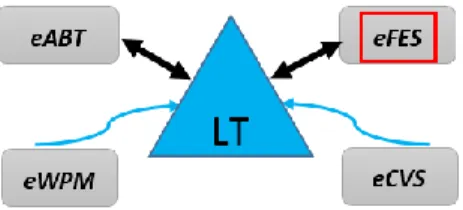
Figure 1. This illustration shows the elevated system externals of eMLEE. Logical Table (LT) interacts primarily with eFES and eABT as compared to the other two modules. It coordinates and regulates the metrics of the learning process in the parallel mode.

Figure 1.This illustration shows the elevated system externals of eMLEE. Logical Table (LT) interacts primarily with eFES and eABT as compared to the other two modules. It coordinates and regulates the metrics of the learning process in the parallel mode.

1.3. Our Contributions

Our contributions are the following.

a. Improved feature search and quantification for unknown or previously unlabeled features in the

datasets for new insights and the relevance of predictive modeling.

b. Outlier identification to minimize the effects on classifier learning.

c. Constructing a feature grouping function (FGF) to add or remove a feature once we have

scored them in their correlation, relevance, and non-redundancy nature of predictive value. Identifying the true nature of the feature vs attribute so bias can be reduced. Features tend to gain or lose their significance (predictive value) from one dataset to another. A perfect example would be an attribute “Gender” (e.g., Gender/Sex may not have any predictive value in a certain type of the dataset/prediction). However, it may have significant value in the different dataset.

d. Constructing a logical 3D space where each feature is observed for its fitness value. Each feature

can be quantified based on a logical point in 3D space. Its contribution towards overfitting (x),

underfitting (y), and optimum-fitting (z) can be scored, recorded, and then weighted for adding

or removing in FGF.

e. Developing a unique approach of utilizing an important metric in ML (i.e., error). We have

trained our model to be governed by maximum and minimum bounds of the error, so we can maintain acceptable bias and fitness including overlearning. Our maximum and minimum bounds for errors are 80% and 20% respectively. These error bounds can be considered one of our novel ideas in the proposed work. The logic goes thus: models are prone to overfitting, bias, high errors, and low accuracy. We tried to envision if the proposed model can be governed by some limits of the errors. Errors above 80% or below 20% are considered red flags. Such may indicate, bias, overlearning or under-learning of the model. Picking 80% and 20% was our rule of thumb to validate our theory with experiments on a diverse dataset (discussed in the appendix).

f. Finally, engineering local gain (LG) and global gain (GG) functions to improve the feature tuning

and optimization.

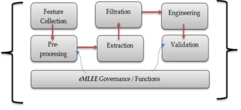
Figure2shows the elevated level block diagram of the eFES Unit.

Appl. Sci. 2018, 8, x 3 of 32

1.3. Our Contributions

Our contributions are the following.

a. Improved feature search and quantification for unknown or previously unlabeled features in the datasets for new insights and the relevance of predictive modeling.

b. Outlier identification to minimize the effects on classifier learning.

c. Constructing a feature grouping function (FGF) to add or remove a feature once we have scored them in their correlation, relevance, and non-redundancy nature of predictive value. Identifying the true nature of the feature vs attribute so bias can be reduced. Features tend to gain or lose their significance (predictive value) from one dataset to another. A perfect example would be an attribute “Gender” (e.g., Gender/Sex may not have any predictive value in a certain type of the dataset/prediction). However, it may have significant value in the different dataset.

d. Constructing a logical 3D space where each feature is observed for its fitness value. Each feature can be quantified based on a logical point in 3D space. Its contribution towards overfitting(x), underfitting (y), and optimum-fitting (z) can be scored, recorded, and then weighted for adding or removing in FGF.

e. Developing a unique approach of utilizing an important metric in ML (i.e., error). We have trained our model to be governed by maximum and minimum bounds of the error, so we can maintain acceptable bias and fitness including overlearning. Our maximum and minimum bounds for errors are 80% and 20% respectively. These error bounds can be considered one of our novel ideas in the proposed work. The logic goes thus: models are prone to overfitting, bias, high errors, and low accuracy. We tried to envision if the proposed model can be governed by some limits of the errors. Errors above 80% or below 20% are considered red flags. Such may indicate, bias, overlearning or under-learning of the model. Picking 80% and 20% was our rule of thumb to validate our theory with experiments on a diverse dataset (discussed in the appendix).

f. Finally, engineering local gain (LG) and global gain (GG) functions to improve the feature tuning and optimization.

Figure 2 shows the elevated level block diagram of the eFES Unit.

Figure 2. eFES elevated Level.

2. Related Study

To identify the gaps in the latest state of the art in the field of FO, we considered area of ML where FO was of high relevance. In general, every ML problem is affected by feature selection and feature processing. Predictive modeling, as our focus for the consumption of the proposed model, is a great candidate to be looked at, for FO opportunities. One of the challenges in FO is to mine the hidden features that are previously unknown and may hide a great predictive value. If such knowledge can be extracted and quantified, ML process can dramatically be improved. On the other hand, new features can also be created by aggregating existing features. Also, two irrelevant features

Figure 2.eFES elevated Level. 2. Related Study

To identify the gaps in the latest state of the art in the field of FO, we considered area of ML where FO was of high relevance. In general, every ML problem is affected by feature selection and feature processing. Predictive modeling, as our focus for the consumption of the proposed model, is a great candidate to be looked at, for FO opportunities. One of the challenges in FO is to mine the hidden features that are previously unknown and may hide a great predictive value. If such knowledge can be extracted and quantified, ML process can dramatically be improved. On the other hand, new features can also be created by aggregating existing features. Also, two irrelevant features can be combined, and their weighted function can become a productive feature with higher predictive value.

Clearly, in-depth comprehensive review of the FO and related state of the art are outside the scope of this paper. However, in this section we provide the related study of noteworthy references and then list the

gaps we identified. We also present the comparisons of some of the techniques in Section5.

Li et al. [3] presented a detailed review of the latest development in the feature selection segment of

machine learning. They provided various frameworks, methods, and comparisons in both Supervised Learning (SL) and Unsupervised Learning (UL). However, their comparative study did not reveal any development where each feature can achieve a run-time predictive scoring and can be added

or removed algorithmically as the learning process continues. Vergara and Estevez [14] reviewed

feature selection methods. They presented updates on results in a unifying framework to retrofit successful heuristic criteria. The goal was to justify the need of the feature selection problem in depth concepts of relevance and redundancy. However, their work was only focused on unifying

frameworks and placed the generalization on broader scale. Mohsenzadeh et al. [15] utilized a sparse

Bayesian learning approach for feature sample selection. Their proposed relevance sample feature machine (RSFM) is an extension of RVM algorithm. Their results showed the improvement in removing irrelevant features and producing better accuracy in classification. Additionally, their results also demonstrated better generalization, less system complexity, reduced overfitting, and computational

cost. However, their work needs to be extended to more SL algorithms. Ma et al. [16] utilized Particle

Swarm Optimization (PSO) algorithm to develop their proposed approach for detection of falling elderly people. Their proposed research enhances the selection of variables (such as hidden neurons, input weights, etc.) The experiments showed higher sensitivity, specificity, and accuracy readings. Their work though in the domain of healthcare industry does not address the application of approach to a different

industry with an entirely different dataset. Lam et al. [17] proposed a unsupervised feature-learning

process to improve the speed and accuracy, using the Unsupervised Feature Learning (UFL) algorithm, and fast radial basis function (RBF) for further feature training. However, the UFL may not fit when

applied. SL. Han et al. [18] used circle convolutional restricted Boltzmann machine method for 3D

feature learning in unsupervised process of ML. The goal was to learn from raw 3D shapes and to overcome the challenges of irregular vertex topology, orientation ambiguity on the surface, and rigid transformation invariances in shapes. Their work using 3D modeling needs to be extended to SL

domains and feature learning. Zeng et al. [19] used the deep perceptual features for traffic sign

recognition in the kernel extreme learning machines. Their proposed DP-KELM algorithm showed high efficiency and generalization. However, the proposed algorithm needs to be tested across different traffic systems in the world for more distinctive features than those they have considered.

Wang et al. [20] discussed the process of purchase decision in subject minds using MRI scanning images

through ML methods. Using the recursive cluster elimination-based SVM method, they obtained higher accuracy (71%) as compared to previous findings. They utilized Filter (GML) and wrapping methods (RCE) for feature selection. Their work also needs to be extended to other image techniques in

healthcare. Lara et al. [21] provided a survey on ML application for wearable sensors, based on human

activity recognition. They provided a taxonomy of learning approach and their related response time on their experiments. Their work also supported feature extraction as an important phase of ML process. ML has also shown a promising role in engineering, mechanical, and thermo-dynamic

systems. Zhang et al. [22] worked on ML techniques to do the prediction in the thermal systems for

systems components. Besides many different units and technique adoptions, they also utilized FS methods based on correlation feature selection algorithm. They used Weka data-mining tools and came up with the reduced feature set of 16 for improved accuracy. However, their study did not reveal how exactly they came up with this number and whether different number of the features would

have helped any further. Wang et al. [23] used the supervised feature method to remove redundant

features and considered the important ones for their gender classification. However, they used the neural network method as a feature extraction method, which is mostly common in unsupervised learning. Their work is yet to be tested for more computer vision tasks including image recognition

F-measure optimization for FS. They developed a cost-sensitive feature approach to determine the best F-measure-based feature for the selection by ML process. They argued F-measure to be better than accuracy, for purposes of performance measurement. However, accuracy is not sufficient to be

considered a baseline for performance reflection of any model or process. Abbas et al. [25] proposed

solutions for IoT-based feature models using the multi-objective optimum approach. They enhanced the binary pattern for nested cardinality constraints using three paths. The second path was observed to increase the time complexity due to the increasing group of features. Though their work was not directly in ML methodologies, their work showed performance improvement in the 3rd path when the optional features were removed.

Here are the gaps that we identified based on a comprehensive literature review and comparisons

made, evaluated, and presented in Section5later in this paper.

a. Parallel processing of the features, in which features can be evaluated one by one, has not been

done, while the model metrics are being measured and recorded simultaneously to see the real-time effect.

b. Improved grouping of features is needed across diverse feature types in datasets for improved

performance and generalization.

c. 3D modeling is rarely done. The 3D approach can help for side-by-side metric evaluation.

d. Accuracy is taken as granted to measure the performance of the model. However, we argue on

the relevance of this metric and support other metrics in conjunction with it. We engineer our model to incline towards the metrics that are found relevant for a given problem based on the classifier learning.

e. Feature quantification and function building governed by algorithms the way we presented

is not found in the literature, and the dynamic ability of such a design, as our work indicated, can be a good filler of this gap in the state of the art.

f. Finally, FO has not been directly addressed. FO helps to regulate the error biasing, outlier

detection, and poor generalization.

3. Groundwork of eFES

This section presents background on the underlying theory, mathematical constructs, definitions, algorithms, and the framework.

The elevated-level framework shown in Figure3elaborates on the importance of each definition,

incorporated with the other units of eMLEE and the ability to implement parallel processing by design. In general computing, parallel processing is done by dividing program instructions to be run by multiple processors, so the time efficiency can be improved. This also ensures the maximum utilization of otherwise idle processors. Similar concepts can be implemented on the algorithms and ML models. ML algorithms depend on the problem and data types and require sequential training of each of the data models. However, the parallel processing can dramatically improve the learning process, especially for the blended model, such as eMLEE. In light of the latest work of parallel processing

in ML, such as in [26], the authors introduced the parallel framework on ML algorithms for large

graphs. They experimented with aggregation and sequential steps in their model to allow researchers

to improve the usage of various algorithms. Another study was done in [27], where authors used

induction to improve the parallelism in the decision trees. Python and R libraries have come a long

way to help provide useful libraries and classes to develop various ML techniques. Authors in [28]

introduced a python library Qjan to parallelize the ML algorithms in compliance by MapReduce.

A PhD thesis [29] work done by a student at the University of California at Berkeley used concurrency

control method to parallelize the ML process. Another study done in [30] utilized parallel processing

approaches in ML techniques for detection in big-data networks. Therefore, similar progresses have motivated us to incorporate parallel processing in the proposed model.

Our proposed model parallelism is done in two layers:

(i) Outer layer to eFES, where eFES unit communicates with other units of the eMLEE such as eABT,

eWPM, eCVS and LT. Parallelism is done through real-time metric measurement with LT object and based on classifier learning, eFES reacts to the inner layer (defined next). Other units such as eABT and eCVS enhance the algorithm blend and test-training split in parallel, while eFES is being trained. In other words, all four units including eFES regulated by LT unit, are run in parallel to improve the speed of the learning process and validation for every feature as processed in the eFES unit and every algorithm processed in the eABT unit. However, eFES can also work without being related to the other units, if researchers and industrialists may however choose so.

(ii) Inner layer to eFES, where adding and removing of the feature are done in parallel. When the

qualifying feature is added, the metrics are measured by the model to see if fitness improves, and then features are added and removed one by one to see the effect on the fitness function. This may be done sequentially, but parallelism improves the insurance that each feature is evaluated at the same time; the classifier is incorporating metrics reading from LT object and speed of the process especially when the huge dataset is being processed.

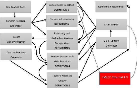
Figure3illustrates the inner layer parallel processing of each construct that constitutes the eFES

unit. It shows the high-level block diagram of eFES unit modeling and related functions. Each definition is explained in plain English next.

Appl. Sci. 2018, 8, x 6 of 32

Our proposed model parallelism is done in two layers:

(i) Outer layer to eFES, where eFES unit communicates with other units of the eMLEE such as eABT, eWPM, eCVS and LT. Parallelism is done through real-time metric measurement with LT object and based on classifier learning, eFES reacts to the inner layer (defined next). Other units such as eABT and eCVS enhance the algorithm blend and test-training split in parallel, while eFES is being trained. In other words, all four units including eFES regulated by LT unit, are run in parallel to improve the speed of the learning process and validation for every feature as processed in the eFES unit and every algorithm processed in the eABT unit. However, eFES can also work without being related to the other units, if researchers and industrialists may however choose so.

(ii) Inner layer to eFES, where adding and removing of the feature are done in parallel. When the qualifying feature is added, the metrics are measured by the model to see if fitness improves, and then features are added and removed one by one to see the effect on the fitness function. This may be done sequentially, but parallelism improves the insurance that each feature is evaluated at the same time; the classifier is incorporating metrics reading from LT object and speed of the process especially when the huge dataset is being processed.

Figure 3 illustrates the inner layer parallel processing of each construct that constitutes the eFES unit. It shows the high-level block diagram of eFES unit modeling and related functions. Each definition is explained in plain English next.

Figure 3. Theoretical Foundation Illustration on the elevated-level.

Definition 1 covers the theory of LT unit, which works as a main coordinator assisting and regulating all the sub-units of eMLEE engine such as eFES. It inherently is based on parallel processing at a low level. While the classifier is in the learning process, LT object (in parallel) performs the measurements, records it, updates it as needed, and then feeds the learning process back. During classifier learning, LT object (governed by LT algorithm, outside of scope of this paper, but will be available as an API) creates a logical table (with rows and columns) where it adds or removes the entry of each feature as a weighted function, while constantly measuring the outcome of the classifier learning.

Definition 2 covers the creation of the feature set from raw input via random process, as shown above. As discussed earlier, it uses 3D modeling using x, y, and z coordinates. Each feature is

Figure 3.Theoretical Foundation Illustration on the elevated-level.

Definition 1 covers the theory of LT unit, which works as a main coordinator assisting and regulating all the sub-units of eMLEE engine such as eFES. It inherently is based on parallel processing at a low level. While the classifier is in the learning process, LT object (in parallel) performs the measurements, records it, updates it as needed, and then feeds the learning process back. During classifier learning, LT object (governed by LT algorithm, outside of scope of this paper, but will be available as an API) creates a logical table (with rows and columns) where it adds or removes the entry of each feature as a weighted function, while constantly measuring the outcome of the classifier learning.

Definition 2 covers the creation of the feature set from raw input via random process, as shown

above. As discussed earlier, it uses 3D modeling usingx,y, andzcoordinates. Each feature is quantized

based on the scoring of these coordinates (xbeing representative of overfit,ybeing underfit andz

Definition 3 covers the core functions of this unit to quantify the scoring of the features, based on their redundancy and irrelevancy. It does this in a unique manner. It should be noted that not every irrelevant feature with high score will be removed by the algorithm. That is the beauty of it. To increase the generalization of such model with a diverse dataset that it has not seen during test (i.e., prediction), features are quantified, and either kept, removed, or put on the waiting list for re-processing of addition or removal evaluation. The benefit of this approach is that it will not do injustice to any feature without giving a second chance later in the learning process. This is because features, once aggregated with a new feature or previously unknown feature, can dramatically improve scores to participate in the learning process. However, the deep work of “unknown feature extraction” is kept for future work, as discussed in the future works section.

Definition 4 utilizes definition 1 to 3 and introduces a global and local gain functions to evaluate the optimum feature-set. Therefore, the predictor features, accepted features, and rejected features can be scored and processed.

Definition 5 finally covers the weight function to observe the 3D weighted approach for each feature that passes through all the layers, before each feature is finally added to the list of the final participating features.

The rest of the section is dedicated to the theoretical foundation of mathematical constructs and underlying algorithms.

3.1. Theory

eFES model manifests itself into specialized optimization goals of the features in the datasets. The most crucial step of all is the Extended Feature Engineering (EFE) that we refer when we build upon existing EF techniques. These five definitions help build the technical mechanics of the proposed model of eFES unit.

Definition 1.Let there be a Logical Table (LT) module that regulates the ML process during eFES constructions. Let LT have 3D coordinates as x, y, and z to track, parallelize, and update the x←overfit(0:1), y←underfit(0:1), z←optimumfit(−1:+1). Let there be two functions, Feature Adder as +F, and Feature Remover as−F, based on linearity of the classifier for each feature under test for which the RoOpF (Rule. 1) is valid. Let Lt. RoOpF > 0.5 to be considered of acceptable predictive value.

eFES LT module builds very important functions at initial layers for adding a good fit feature and removing a bad fit feature from the set of features available to it, especially when algorithm blend is being engineered. Clearly, not all features will have an optimum predictive value and thus identifying them will count towards optimization. The feature adder function is built as:

+F(x,y,z) = +FFn = (Fn∪ Fn+1) Z

∑

(LT.score(i)) +

∑

−_F(x,y,z) =−_FFn = (Fn∩ Fn+1)

x,y

∑

(LT.score(j,k))−

∑

Very similar tok-means clustering [12] concept, that is highly used in unsupervised learning,

LT implements feature weights mechanism (FWM) so it can report a feature with high relevancy score and non-redundant in a quantized form. Thus, we define:

FW M(X,Y,Z) = X

∑

∑

∑

∆(x,y,z) =      ∏L l=1(ulxwlx), ifz 6= 0, AND z > (0.5, y) ui ∈ {0, 1}, −1 ≤ i ≤ L ∏L

l=1(ulywly), ifz 6= 0, AND z > (0.5, x)

(4)

Illustration in Figure4shows the concept of LT modular elements in 3D space as discussed earlier.

Figure5shows the variance of the LT. Figure6shows that it is based on binary weighted classification

scheme to identify the algorithm for blending and then assign a binary weight accordingly in LT logical blocks. The diamond shape shows the err distribution that is observed and recorded by LT module as new algorithm is added or existing is removed. The complete mathematical model for eFES LT is beyond the scope of this paper. We finally provide the eFES LT functions as:

eFES= [_ReFES = 1 Ne r err err + Err 2 ] × N

∑

whereerr= local error (LE),Err= global error (GE).f (x,y,z) is the main feature set in ‘F’ for 3D.

RULE 1

If (LTObject.ScoFunc (A (i) > 0.5) Then

Assign “1” Else Assign “0”

PROCEDURE 1

Execute LT.ScoreMetrics (Un.F, Ov.F)

Compute LT.Quantify (*LT)

Execute LT.Bias (Bias.F, *)

*_Shows the pointer to the LT object.

Definition 2.Fn={F1, F2, F3,. . . , Fn}indicates all the features appears in the dataset, where each feature Fi∈Fn|fw≥0. fwindicates the weighted feature value in the set. Let Fran(x,y,z)indicates the randomized feature set.

We estimate the cost function based on randomized functions. Las Vegas and Monte Carlo algorithms are popular randomized algorithms. The key feature of the Las Vegas algorithm is that it will eventually have to make the right solution. The process involved is stochastic (i.e., not deterministic) and thus guarantee the outcome. In case of selecting a function, this means the algorithm must produce the smallest subset of optimized functions based on some criteria, such as the accuracy of the classification. Las Vegas Filter (LVS) is widely used to achieve this step. Here we set a criterion in which

we expect each feature at random gets a random maximum predictive value in each run. ∅shows

the maximum inconsistency allowed per experiment. Figure5shows the cost function variation in LT

object for each coordinate.

PROCEDURE 2

Scorebest ← Import all attributes as ‘n’ Costbest ← n

For j ← 1~to Iterationmax Do

Cost ← Generate random number between 0~and Costbest

Score ← Randomly select item from Cost feature

If LT.InConsistance (Scorebest, Training Set) ≤ ∅ Then Scorebest ← Score

Costbest ← C Return (Scorebest)

Definition 3.Let lt.IrrF and lt.RedF be two functions to store the irrelevancy and redundancy score of each feature for a given dataset.

Let us define a Continuous Random VectorCRV∈QN, and Discrete Random VariableDRV∈H=

{h1,h2,h3, . . . ..,hn}. The density function of the random vector based on cumulative probability is

P(CRV) =Appl. Sci. ∑N_i=2018, ₁PH8(, x hi)p CRV|DRV,PH(hi) being a priori probability of class. 9 of 32

Figure 4. Illustration of the conceptual view of LT Modules in 3D space.

(a) (b)

(c) (d)

Figure 5. (a) This test shows the variance of the LT module for the cost function for all three co-ordinates and then z (optimum-fitness). This is the ideal behavior; (b) This test shows the real (experimental) behavior; (c) This shows the ideal shift of all 3 coordinates in space while they are tested by the model in parallel. Each coordinate (x, y, z) lies on the black lines in each direction. Then, based on the scoring reported by LT object (and cost function), they either sit on positive point or negative as shown; (d) This shows the ideal spread of each point, when z is optimized with the lowest cost function.

Figure 6. Illustration of probability-based feature binary classification. Overlapped matrices for Red.F

and Irr.F, for which the probability scope resulted in acceptable errors by stepping into vector space,

for which 0.8 > err > 0.2.

Figure 4.Illustration of the conceptual view of LT Modules in 3D space.

Appl. Sci. 2018, 8, x 9 of 32

Figure 4. Illustration of the conceptual view of LT Modules in 3D space.

(a) (b)

(c) (d)

Figure 5. (a) This test shows the variance of the LT module for the cost function for all three co-ordinates and then z (optimum-fitness). This is the ideal behavior; (b) This test shows the real (experimental) behavior; (c) This shows the ideal shift of all 3 coordinates in space while they are tested by the model in parallel. Each coordinate (x, y, z) lies on the black lines in each direction. Then, based on the scoring reported by LT object (and cost function), they either sit on positive point or negative as shown; (d) This shows the ideal spread of each point, when z is optimized with the lowest cost function.

Figure 6. Illustration of probability-based feature binary classification. Overlapped matrices for Red.F

and Irr.F, for which the probability scope resulted in acceptable errors by stepping into vector space,

for which 0.8 > err > 0.2.

Figure 5.(a) This test shows the variance of the LT module for the cost function for all three co-ordinates and then z (optimum-fitness). This is the ideal behavior; (b) This test shows the real (experimental) behavior; (c) This shows the ideal shift of all 3 coordinates in space while they are tested by the model in parallel. Each coordinate (x,y,z) lies on the black lines in each direction. Then, based on the scoring reported by LT object (and cost function), they either sit on positive point or negative as shown; (d) This shows the ideal spread of each point, whenzis optimized with the lowest cost function.

Appl. Sci. 2018, 8, x 9 of 32

Figure 4. Illustration of the conceptual view of LT Modules in 3D space.

(a) (b)

(c) (d)

Figure 5. (a) This test shows the variance of the LT module for the cost function for all three co-ordinates and then z (optimum-fitness). This is the ideal behavior; (b) This test shows the real (experimental) behavior; (c) This shows the ideal shift of all 3 coordinates in space while they are tested by the model in parallel. Each coordinate (x, y, z) lies on the black lines in each direction. Then, based on the scoring reported by LT object (and cost function), they either sit on positive point or negative as shown; (d) This shows the ideal spread of each point, when z is optimized with the lowest cost function.

Figure 6. Illustration of probability-based feature binary classification. Overlapped matrices for Red.F

and Irr.F, for which the probability scope resulted in acceptable errors by stepping into vector space,

for which 0.8 > err > 0.2.

Figure 6.Illustration of probability-based feature binary classification. Overlapped matrices forRed.F andIrr.F, for which the probability scope resulted in acceptable errors by stepping into vector space, for which 0.8 > err > 0.2.

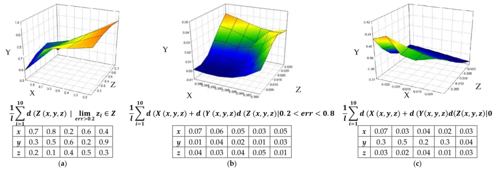
As we observe that the higher error limit (e) (err, green line, round symbol) and lower error limit (E), (Err, blue line, square symbol) bound the feature correlation in this process. Our aim is to spread the distribution in z-dimension for optimum fitting as features are added. The red line (diamond symbol) that separates the binary distribution of Redundant Feature (Red.F) and Irrelevant Features (Irr.F) based on error bounds. The green and red lines define the upper and lower limit of the error, in which all features

correlate. Here, we build a mutual information (MI) function [14] so we can quantify the relevance of a

feature upon other in the random set and this information is used to build the construct forIrr.F, since once

our classifier learns, it will mature theIrr.Flearning module as defined in the Algorithm 1.

MI(Irr.F(x,y,z)|fi,fi+1= N ∑ a=1 N ∑ b=1 p(fi(a),fi+1(b).log _f i(a),fi+1(b) p(fi(a).fi+1(b) (6)

We expectMI←0, for features to be statistically independent, so we build the construct in which

the MI will be linearly related to the entropies of the features under test forIrr.FandRed.F, thus:

M.I(fi, fi+1) =      H(fi)−H(fi|fi+1) H(fi+1−H(fi+1|fi) H(fi) + H(fi+1)−H(fi,fi+1) (7)

We use the following construct to develop the relation of ‘Irr.F’ and ‘Red.F’ to show the irrelevancy

factor and Redundant factor based on binary correlation and conflict mechanism as illustrated in above table. Irr.F=_∑K i,j ( fii fij fji fji ) Red.F=     

MI(fi; Irr.F)>0.5 Strong Relevant Feature

MI(fi; Irr.F)<0.5 Weak Relevant Feature

MI(fi;Irr.F) =0.5 Neutral Relevant Feature

(8)

Definition 4.Globally in 3-D space, there exist three types of features types (variables), as predictor features:

PF = {p f1,p f2,p f3, . . . ..p fn},and accepted features to be AF = {a f1,a f2,a f3, . . . ..,a fn}and

rejected features to be RF={r f1,r f2,r f3, . . . ..r fn},in whichG ≥ (g+1),global gain for all experimental occurrence of data samples. ‘G’being the global gain (GG). ‘ g’being the local gain (LG). Let PV be the predictive value. Accepted features are a fn ∈ PV , strongly relevant to the sample data set∆S,if there exist at-least one x and z or y and z plane with score≥ 0.8 , AND a single feature f ∈ F is strongly relevant to the objective Function ‘ObF’ in distribution ‘d’ if there exist at-least a pair of example in data set

{∆S1,∆S2, ∆S3, . . . .,∆Sn ∈ I},such that d(∆Si) 6= 0and d(∆Si+1) =6 0. Let∇(ϕ,ρ,ω)correspond

to the acceptable maximum 3-axis function for possible optimum values of x, y, and z respectively.

We need to build an ideal classifier that learns from data during training and estimate the predictive

accuracy, so it generalizes well on the testing data. We can use probabilistic theory of Bayesian [31] to

develop a construct similar to direct table lookup. We assume a random variable to be ‘rV’ that will appear

with many values in set of{rV1,rV2,rV3, . . . , rVn}that appear as a class. We will use prior probability

P(rVi). Thus, we represent a class or set of classes asrVi, and the greatestP(rVi), for given pattern of

evidence (pE) that classifier learns on P(rVi

pE) > P(rV_j

pE) valid for all i 6= j.

Because we know that

P(rVi|pE) = P(pE|rVi)P(rVi)

(P(pE)) (9)

Therefore, we can write the conditional equation where P (pE) is considered with regard to

probability of (pE) is P(pErV_i)P(rVi) > P(pE

rVj)P rV_j

valid for all i 6= j. Finally, we can

write the probability of the error for the above given pattern, as P (pE)|error, assuming the

cost function for all correct classification is 0, and for all incorrect is 1, then as stated earlier, the Bayesian classification will put the instance in the class labelling the highest posterior probability

as P (pE) = ∑k

i=1

P(pE)|error = Error[1−max{P(rV1)|pE, . . . ,P(rVk|pE)}]. Let us construct the matrix function

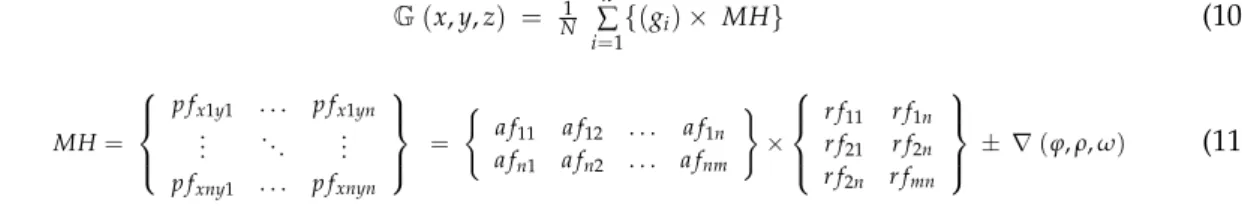
of all features, accepted and rejected features, based on GG and LG, as

G(x,y,z) = _N1 n ∑ i=1 {(gi)× MH} (10) MH=      p fx1y1 . . . p fx1yn .. . . .. ... p fxny1 . . . p fxnyn      = ( a f11 a f12 . . . a f1n a fn1 a fn2 . . . a fnm ) ×      r f11 r f1n r f21 r f2n r f2n r fmn      ± ∇(ϕ,ρ,ω) (11)

Table1shows the various ranges for Minimum, Maximum and Middle points of the all three

functions as discussed earlier.

Table 1.Typical observations of the functions.

Function Min Mid Max

∇(ϕ,ρ,ω) (0.21, 0.71, 0.44) (0.43, 55, 49) (0.81, 0.76, 58)

g(x,y,z) (0.34, 0.51,−0.11) (0.55, 0.51, 0.68) (0.67, 71, 89) G(x,y,z) (0.44, 0.55, 0.45) (0.49, 0.59, 0.58) (0.52, 0.63, 0.94)

Using Naïve Bayes multicategory equality as:

P1,2,3,...,N " ∑ j xj # + " ∑ j yj # + " ∑ j zj # = _∑ k Var(x,y,z) z∗i (12) wherez∗(n)argmax z P(z) _∏n k=1

p([z]).zk, and Fisher score algorithm [3] can be used in FS to measure

the relevance of each feature based on Laplacian score, such thatB(i,j) =

( ₁

N_l i f ui = ui =1

0otherwise, .

Nlshows the no. of data samples in test class shown subscript ‘l’. Generally, we know that based

on specific affinity matrix,FISHERscore(fi) =1− _{LAPCLACI AN}1 _score(fi).

To group the features based on relevancy score, we must ensure that each group member of the features exhibit low variance, medium stability and their score is based on optimum-fitness, thus

each member followsk(k ∈ K, where K ≤ f (0 : 1). This also ensure that we address the high

dimensionality issue, as when feature appears in high dimension, they tend to change their value for training mode, thus, we determine the information gain using entropy function as:

Entropy(Fn) =

V1

∑

t=1

−ptlog pt (13)

V1indicates the number of various value of the target features in set ofF. andptis the probability

of the type of value of t in a complete subset of the feature tested. Similarly, we can calculate the

entropy for each feature inx,y,zdimension as:

Entropy Fn∈x,y,z = ∑

t∈T(x,y,z)

|F(t:x,y,z)|

|Ft| Entropy(Fn) (14)

Consequently, gain function in probability of entropy in 3D is determined as:

GainI, F(t:x,y,z)

= Entropy(Fn) − Entropy Fn∈x,y,z (15) We develop a ratio of gain for each feature in z-dimension as this ensure the maximum fitness of the feature set for the given predictive modeling in the given dataset for which ML algorithm needs to

be trained. Thus,gRindicates the ratio between:

gR(z) = Gain(I,F(t:x,y,z))

Figure7shows the displacement of the local gain and global gain functions based on probability distributions. As discussed earlier, LG and GG functions are developed to regulate the accuracy and

thus validity of the classifier is measured initially based on accuracy metric._{Appl. Sci. 2018, 8, x 12 of 32}

Figure 7. Illustration on probability of LG and GG function.

Table 2 shows the probability of local and global error limits based on probability function (Figure 7) in terms of local (g) and global gain function (G).

Table 2. Typical observations.

g (max) G (min) G (max) g (min) P (err) 0.25 0.45 0.31 0.56 P (Err) 0.32 0.41 0.49 0.59

RULE 2

If (g (err) < 0.2) Then

Flag ‘O.F’

Elseif (g (err) > 0.8) Flag ‘U.F’

If we assume the fact of {∆𝑆1, ∆𝑆2, ∆𝑆3, . . . , ∆𝑆𝑛 ∈ 𝐼}, such that d (∆𝑆𝑖) ≠ 0and d (∆𝑆𝑖+1) ≠ 0, where ‘I’ is the global input of testing data. We also confirm the relevance of the feature in the set using objective Function construct in distribution ‘d’, thus:

𝑂𝑏𝐹 (𝑑, 𝐼) = 𝑙𝑜𝑔 (𝐺𝑎𝑖𝑛 (𝐼, 𝐹 (𝑡:𝑥,𝑦,𝑧)))

(𝑒𝑟𝑟[𝑚𝑎𝑥: 1], 𝑒𝑟𝑟[𝑚𝑖𝑛: 0]) | 𝑑 (∆𝑆𝑖) ≠ 0 | 𝑓𝑜𝑟 𝑒𝑣𝑒𝑟𝑦 𝐹𝑖 𝑖𝑛 𝑔𝑟𝑜𝑢𝑝 (17)

Then, Using Equations (14)–(17), we can finally get

𝐹. 𝐸𝑛𝑔(𝑥, 𝑦, 𝑧) = 1 (𝑘 × 𝑀) ∑ ∏ 𝑂𝑏𝐹 (𝑑, 𝐼) × 𝑀 𝑡=𝑘 𝐾 𝑡=1 𝑀𝐻𝑡) (18) 𝐹. 𝐺𝑟𝑝(𝑥, 𝑦, 𝑧) = 𝐹. 𝐸𝑛𝑔(𝑥, 0,0) + 𝐹. 𝐸𝑛𝑔(0, 𝑦, 0) − 𝐹. 𝐸𝑛𝑔(0,0, 𝑧) (19) Figure 8 Illustration of Feature Engineering and Feature Group as constructed in the mathematical model and governed by the Algorithms 1 and 2, defined later. Metrics API is available from eMLEE package. The white, yellow, and red orbital shapes indicate the local gain progression through 3D space. The little 3D shapes (x, y, and z) in the accepted feature space in grouping indicates several (theoretically unlimited) instances of the optimized values as the quantization progresses.

Figure 8. Illustration of Feature Engineering and Feature Group as constructed in the mathematical model.

Figure 7.Illustration on probability of LG and GG function.

Table2shows the probability of local and global error limits based on probability function

(Figure7) in terms of local (g) and global gain function (G).

Table 2.Typical observations. g (max) G (min) G (max) g (min) P (err) 0.25 0.45 0.31 0.56 P (Err) 0.32 0.41 0.49 0.59

RULE 2

If (g (err) < 0.2) Then Flag ‘O.F’

Elseif (g (err) > 0.8) Flag ‘U.F’

If we assume the fact of {∆S1,∆S2, ∆S3, . . . .,∆Sn ∈ I} , such that d (∆Si) 6= 0 and d

(∆Si+1) 6= 0 , where ‘I’ is the global input of testing data. We also confirm the relevance of the

feature in the set using objective Function construct in distribution ‘d’, thus:

ObF(d, I) =log(Gain(I,F(t:x,y,z)))

(err[max:1],err[min:0]) |d(∆Si) 6= 0| f or every Fiin group (17) Then, Using Equations (14)–(17), we can finally get

F.Eng(x,y,z) = _(k×1_{M) ∑}K t=1 M ∏ t=k ObF(d,I)×MHt) (18)

F.Grp(x,y,z) = F.Eng(x, 0, 0) + F.Eng(0,y, 0)−F.Eng(0, 0,z) (19)

Figure8Illustration of Feature Engineering and Feature Group as constructed in the mathematical

model and governed by the Algorithms 1 and 2, defined later. Metrics API is available from eMLEE package. The white, yellow, and red orbital shapes indicate the local gain progression through 3D

space. The little 3D shapes (x,y, andz) in the accepted feature space in grouping indicates several

(theoretically unlimited) instances of the optimized values as the quantization progresses.

Appl. Sci. 2018, 8, x 12 of 32

Figure 7. Illustration on probability of LG and GG function.

Table 2 shows the probability of local and global error limits based on probability function (Figure 7) in terms of local (g) and global gain function (G).

Table 2. Typical observations.

g (max) G (min) G (max) g (min) P (err) 0.25 0.45 0.31 0.56 P (Err) 0.32 0.41 0.49 0.59

RULE 2

If (g (err) < 0.2) Then

Flag ‘O.F’

Elseif (g (err) > 0.8) Flag ‘U.F’

If we assume the fact of {∆𝑆1, ∆𝑆2, ∆𝑆3, . . . , ∆𝑆𝑛 ∈ 𝐼}, such that d (∆𝑆𝑖) ≠ 0and d (∆𝑆𝑖+1) ≠ 0, where ‘I’ is the global input of testing data. We also confirm the relevance of the feature in the set using objective Function construct in distribution ‘d’, thus:

𝑂𝑏𝐹 (𝑑, 𝐼) = 𝑙𝑜𝑔 (𝐺𝑎𝑖𝑛 (𝐼, 𝐹 (𝑡:𝑥,𝑦,𝑧)))

(𝑒𝑟𝑟[𝑚𝑎𝑥: 1], 𝑒𝑟𝑟[𝑚𝑖𝑛: 0]) | 𝑑 (∆𝑆𝑖) ≠ 0 | 𝑓𝑜𝑟 𝑒𝑣𝑒𝑟𝑦 𝐹𝑖 𝑖𝑛 𝑔𝑟𝑜𝑢𝑝 (17) Then, Using Equations (14)–(17), we can finally get

𝐹. 𝐸𝑛𝑔(𝑥, 𝑦, 𝑧) = 1 (𝑘 × 𝑀) ∑ ∏ 𝑂𝑏𝐹 (𝑑, 𝐼) × 𝑀 𝑡=𝑘 𝐾 𝑡=1 𝑀𝐻𝑡) (18) 𝐹. 𝐺𝑟𝑝(𝑥, 𝑦, 𝑧) = 𝐹. 𝐸𝑛𝑔(𝑥, 0,0) + 𝐹. 𝐸𝑛𝑔(0, 𝑦, 0) − 𝐹. 𝐸𝑛𝑔(0,0, 𝑧) (19) Figure 8 Illustration of Feature Engineering and Feature Group as constructed in the mathematical model and governed by the Algorithms 1 and 2, defined later. Metrics API is available from eMLEE package. The white, yellow, and red orbital shapes indicate the local gain progression through 3D space. The little 3D shapes (x, y, and z) in the accepted feature space in grouping indicates several (theoretically unlimited) instances of the optimized values as the quantization progresses.

Figure 8. Illustration of Feature Engineering and Feature Group as constructed in the mathematical model.

Definition 5. Feature selection is governed by satisfying the scoring function (score) in 3D space (x: Over-Fitness, y: Under-Fitness, z: Optimum-Fitness) for which evaluation criterion needs to be maximized, such that Evaluation Criterion: f0. There exist a weighted, W(∅){∇(ϕ,ρ,ω), 1}function that quantifies the score for each feature, based on response from eMLEE engine with function eMLEEreturn, such that each feature in{f1, f2, f3, . . . .., fn,}, has associated score for(ϕ:x,y,z,ρ:x,y,z,ω:x,y,z).

Two or more features may have the same predictive value and will be considered redundant. The non-linear relationship exists between two or more features (variables) that affects the stability and linearity of the learning process. If the incremental accuracy is improved, then non-linearity of a variable is ignored. As the number of the features are added or removed in the given set, the OF, UF, and B changes. Thus, we need to quantify their convergence, relevance, and covariance distribution

across the space in 3D. We implement weighted function for each metric using LVQ technique [1],

in which, we measure each metric over several experimental runs for enhanced feature set, as reported back from the function explained in Theorems 1 and 2, such that we optimize the z-dimension for

optimum fitness and reducexandydimension for over-fitness and under-fitness. Let us define:

W(∅) = R 1 Stp(x)dx σ ∑ γ=1 NT γ.Nγ R Sγ p(x)dx (20)

where the piecewise effective decision border isSt = _∑σ

γ=1

Sγ , In addition, the unit normal vector,

(Nγ) for borderSγ, γ=1, 2, 3, 4, . . . .σis valid for all cases in space. Let us define the probability

distribution of data onSγ : Qγ=

R

Sγ

p(x)dx. Here, we can use the Parzen method [32], to restore the

nonparametric density estimation method, to estimate theQγ.

d Qγ(∆) = K ∑ j=1 δ(d(xi, Sγ) ≤ ∆2 (21)

where d (xi, Sγ)shows the Euclidean distance function. Figure9shows the Euclidean distance

function based on binary weights forW(∅)function.

Appl. Sci. 2018, 8, x 13 of 32

Definition 5.Feature selection is governed by satisfying the scoring function (score) in 3D space (x:

Over-Fitness, y: Under-Over-Fitness, z: Optimum-Fitness) for which evaluation criterion needs to be maximized, such that 𝐸𝑣𝑎𝑙𝑢𝑎𝑡𝑖𝑜𝑛 𝐶𝑟𝑖𝑡𝑒𝑟𝑖𝑜𝑛: 𝑓′. There exist a weighted, 𝑊(∅){𝛻(𝜑, 𝜌, 𝜔), 1} function that quantifies the score for each feature, based on response from eMLEE engine with function 𝑒𝑀𝐿𝐸𝐸𝑟𝑒𝑡𝑢𝑟𝑛, such that each

feature in {𝑓1, 𝑓2, 𝑓3, … … . . , 𝑓𝑛, }, has associated score for (𝜑: 𝑥, 𝑦, 𝑧, 𝜌: 𝑥, 𝑦, 𝑧, 𝜔: 𝑥, 𝑦, 𝑧).

Two or more features may have the same predictive value and will be considered redundant. The non-linear relationship exists between two or more features (variables) that affects the stability and linearity of the learning process. If the incremental accuracy is improved, then non-linearity of a variable is ignored. As the number of the features are added or removed in the given set, the OF, UF, and B changes. Thus, we need to quantify their convergence, relevance, and covariance distribution across the space in 3D. We implement weighted function for each metric using LVQ technique [1], in which, we measure each metric over several experimental runs for enhanced feature set, as reported back from the function explained in Theorems 1 and 2, such that we optimize the z-dimension for optimum fitness and reduce x and y dimension for over-fitness and under-fitness. Let us define:

𝑊(∅) = 1 ∫ 𝑝(𝑥)𝑑𝑥_𝑆 𝑡 ∑ 𝑁𝛾𝑇 . 𝑁𝛾 ∫ 𝑝(𝑥)𝑑𝑥 𝑆𝛾 𝜎 𝛾=1 (20) where the piecewise effective decision border is 𝑆𝑡= ∑𝜎𝛾=1𝑆𝛾, In addition, the unit normal vector,

(𝑁𝛾) for border 𝑆𝛾, 𝛾 = 1, 2, 3, 4, … … . 𝜎 is valid for all cases in space. Let us define the probability

distribution of data on 𝑆𝛾∶ ℚ𝛾= ∫ 𝑝(𝑥)𝑑𝑥._𝑆𝛾 Here, we can use the Parzen method [32], to restore the

nonparametric density estimation method, to estimate the ℚ𝛾.

ℚ̂ (∆) = ∑ 𝛿 (𝑑 (𝑥𝛾 𝑖 𝐾 𝑗=1 , 𝑆𝛾) ≤ ∆ 2 (21)

where 𝑑 (𝑥𝑖, 𝑆𝛾) shows the Euclidean distance function. Figure 9 shows the Euclidean distance

function based on binary weights for 𝑊(∅) function.

Figure 9. Illustration of function based on Euclidean Distance function.

Table 3 lists the quick comparison of the values of two functions as developed to observe the minimum and maximum bounds.

Table 3. Average Observations.

Function Min Max

𝑊(∅) _{28.31% 78.34%}

ℚ𝜸 +0.2834 −0.1893

We used the Las Vegas Algorithm approach that helps to get correct solution at the end. We used it to validate the correctness of our gain function. This algorithm guarantees correct outcome if the solution is returned or created. It uses the probability approximate functions to implement runnable time-based instances. For our feature selection problem, we will have a set of features that will guarantee the optimum minimum set of features for acceptable classification accuracy. We use linear regression to compute the value of features to detect the non-linearity relationship between

Figure 9.Illustration of function based on Euclidean Distance function.

Table3lists the quick comparison of the values of two functions as developed to observe the

minimum and maximum bounds.

Table 3.Average Observations. Function Min Max

W(∅) 28.31% 78.34% Qγ +0.2834 −0.1893

We used the Las Vegas Algorithm approach that helps to get correct solution at the end. We used it to validate the correctness of our gain function. This algorithm guarantees correct outcome if the solution is returned or created. It uses the probability approximate functions to implement runnable time-based instances. For our feature selection problem, we will have a set of features that

will guarantee the optimum minimum set of features for acceptable classification accuracy. We use linear regression to compute the value of features to detect the non-linearity relationship between

features, we thus implement a function,Func(U(t)) =a+b∗t. Where a, and b are two test features

and values can be determined by using linear regression techniques, so b = ∑

T t=1(t−t)(U(t)−u) ∑T t=1(t−t) 2 . Where,a= u−b∗ t,u= 1_T ∑T t=1 U(t),t= _T1 ∑T t=1

t. These equations also minimize the squared error.

To compute weighted function, we use feature ranking technique [12]. In this method, we will score

each feature, based on quality measure such as information gain. Eventually, the large feature set will be reduced to a small feature set that is usable. The Feature Selection can be enhanced in several ways such as pre-processing, calculating information gain, error estimation, redundant feature or terms removal, and determining outlier’s quantification, etc. The information gain can be determined as:

GainI(w) = − M ∑ j=1 P(Mj). logP(Mj) +P(w) M ∑ j=1 P(Mj|w). logP(Mj|w) +P(w) M ∑ j=1 P(Mj|w). logP(Mj|w) (22)

‘M’ shows the number of classes and ‘P’ is the probability. ‘W’ is the term that it contains as

a feature.P Mjw) is the conditional probability. In practice, the gain is normalized using Entropy,

such as

Norm.GainI(w) =n {GainI(w)}

−n(w)

n log n(w)

n

o (23)

Here we apply conventional variance-mean techniques. We can assume, max∇ ∑n

i=1ϕiρiωi− ∑n

i=1logϕiρiωi. The algorithm will ensure that ‘EC{F.Sco(x, y, z), F.Opt(x, y, z) ≥ 0.5}’ stays in

optimum bounds. Linear combination of Shannon information terms [7] and conditional mutual

information maximization (CMIM) [3] for UMAX(Zk) = max

Zk∈∆s

[Inf(Z_k : X, Y|(XY)_k)] builds the

functions as Score(X|Y) = _∑ yk∈Y G(yk). ∑ xk0∈X G(xk0) ×log(g(z)) (24) JMI N(Z)d= −β( K(0) ∏ k,k0 S(X:Y)_k+ γ( K(0) ∏ k,k0 S(Y:X)_k0 (25)

By using Equations (23)–(27), we get

F.Sco(x,y,z) = Score(X|Y) + _∑n i=1 W(∅)i−∑jn=1Gainj(w) (26) F.Opt(x,y,z) = JMI N(Z)d. N ∏ F.Soc(x,y,z) n _F.Soc(x,y,z) 1+TNorm.GainI(w) o −_∑n j=1∆ Err(j) (27) 3.2. eFES Algorithms

The following algorithms aim: (i) to compute functions as raw feature extraction, related features identification, redundancy, and irrelevancy to prepare the layer for feature pre-processing; (ii) to compute and quantify the selection and grouping factor for the acceptance as model incorporates them; and (iii) to compute the optimization function of the model, based on weights and scoring functions. objeMLEEis the API call for accessing public functions

Following are the pre-requisites for the algorithms.

Initialization: Set the algorithm libraries, create subset of the dataset for random testing and then correlating (overlapping) tests.

Create:LTObjectfor eFES

Create: ObjeMLEE (h)/*create an object reference of eMLEE API */

Set: ObjeMLEE.PublicFunctions (h.eABT,h.eFES,h.eWPM,h.eCVS)/* Handles for all four constructs*/

Dataset Selection: These algorithms require the dataset to be formatted and labelled with supervised learning in mind. These algorithms have been tested for miscellaneous datasets selected from different domains as listed in the appendix. Some preliminary clean-up may be needed depending upon the sources and raw format of the data. For our model building, we developed a Microsoft SQL Server-based data warehouse. However raw data files such as TXT and CSV are valid input files.

Overall Goal (Big Picture): The foremost goal of these two algorithms is to govern the mathematical model built-in eFES unit. These algorithms are essential to work in a chronological mode, as the output of Algorithm 1 is required for Algorithm 2. The core idea that algorithms utilize is to quantify each feature either in original, revealed or an aggregated state. Based on such scoring, which is very dynamic and parallelized while classifier learning is being governed by these algorithms, the feature is removed, added, or put on the waiting list, for the second round of screening. This is the beauty of it. For example, Feature-X may be scored low in the first round and because Feature-Y is now added, that impacts the scoring of the Feature-X, and thus Feature-X is upgraded by scoring function and included accordingly. Finally, algorithms accomplish the optimum grouping of the features from the dataset. This scheme maximizes the relevance, reduces the redundancy, improves the fitness, accuracy, and generalization of the model for improved predictive modeling in any datasets.

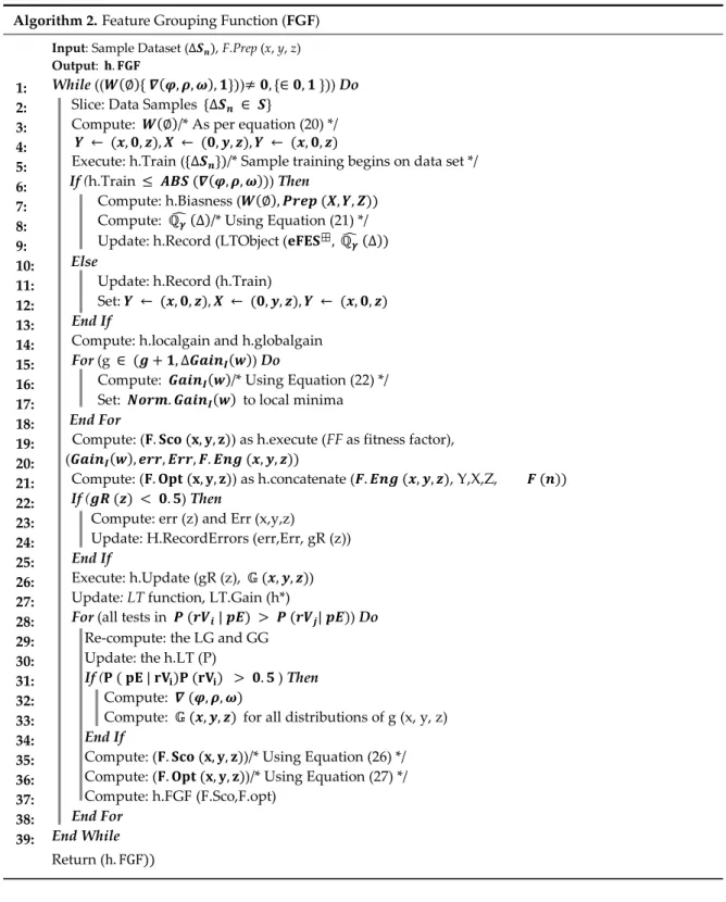
Algorithm 1 aims to compute the low-level function asF.Prep(x,y,z), based on final Equations (26)

and (27) as developed in the model earlier. It uses the conditions of Irrelevant feature and Redundant feature functions and run the logic if the values are below 50% as a check criterion. This algorithm splits the training data based on popular approach as cross validation. However, it must be noted in

line 6, that we use our model API for improving the value ofkin the process, that we call enhanced

cross validation. LT object regulates it and optimizes the value ofkbased on the classifier performance

in the real time. It then follows the error rule (80%, 20%) and keeps track of each corresponding feature, as they are added or removed. Finally, it gets to the start using the gain function in 3D space for each fitting factor since our model is based on 3D scoring of each feature in the space where point is moved

inx,y, andzvalues in space (logical tracking during classifier learning).

Algorithm 2 aims to use the output of algorithm 1 in conjunction with computing many other crucial functions to compute a final function of feature grouping function (FGF). It uses the weighted function to analyze each participating feature including the ones that were rejected. It also utilizes the LT object and its internal functions using the API. This algorithm slices the data into various non-overlapping segments. It uses one segment at a time, then randomly mixed them for more slices

to improve the classifier generalization ability during the training phase. It uses eFESas a LT object

from the library of eMLEE and records the coordinates for each feature. This way, entry is made in LT class, corresponding to the gain function as shown in lines 6 to 19. From line 29 to 35, it also uses

probability distribution function, as explained earlier. It computes two crucial functions of∇(ϕ,ρ,ω)

andG(x,y,z). For this global gain (GG) function, each distribution of local gaing(x,y,z) must be

considered as features come in for each test. All the low probability-based readings are discarded for active computation but kept in waiting list in the LT object for the second run. This way, algorithm does justice to each feature and give it a second chance before finally discarding it. The rest of the features that qualify in first or second run, are then added to the FGF.

Example 1. In one of the experiments (such as Figure 13) on dataset with features including ‘RELIGION’, we discovered something very interesting and intuitive. The data was based on survey from students, as listed in the appendix. We then formatted some of the sets from different regions and ran our Good Fit Student (GFS) and Good Fit job Candidate (GFjC) algorithms (as we briefly discuss in future works). GFS and GFjC are based on eMLEE model and utilize eFES. We noticed as a pleasant surprise that in some cases, it rejected the RELIGION feature for GFS prediction and this made sense as normally religion will not influence success in the studies of the student, but then we discovered that it gave some acceptable scoring to the same feature, because it was coming from a different GEOGRAPHICAL region of the world. It made sense as well, because religion’s influence on the individual may be diverse depending on his or her background. We noticed that it successfully correlated with Correlation Factor (CF) > 0.83 on other features in the set and considered the associated feature to be given high