1574-8936/12 $58.00+.00 © 2012 Bentham Science Publishers
Data Preprocessing and Filtering in Mass Spectrometry Based Proteomics
Beáta Reiz
1,2,3, Attila Kertész-Farkas
1, Sándor Pongor
1,2and Michael P. Myers*
,11International Centre for Genetic Engineering and Biotechnology, 34012 Trieste, Italy, 2Szeged Biological Center, Temesvári krt 67, Szeged, Hungary, 6720 3Institute of Informatics, University of Szeged, Aradi vértanúk tere 1, Szeged, Hungary, 6720
Abstract: Mass spectrometry based proteomics analysis can produce many thousands of spectra in a single experiment, and much of this data, frequently greater than 50%, cannot be properly evaluated computationally. Therefore a number of strategies have been developed to aid the processing of mass spectra and typically focus on the identification and elimination of noise, which can provide an immediate improvement in the analysis of large data streams. This is mostly carried out with proprietary software. Here we review the current main principles underlying the preprocessing of mass spectrometry data give an overview of the publicly available tools.
Keywords: Data filtering, Mass spectrometry, Proteomics.
1. INTRODUCTION
Mass spectrometry coupled with high performance liquid chromatography has become the de facto experimental standard for the proteomic analysis of complex biological materials such as tissue samples, biofluids, immunoprecipitates etc. [1]. Each sample produces several thousand spectra, and owing to the large amount and complexity of the data, interpretation of LC-MS/MS relies almost entirely on computational tools [2]. Despite recent technological advances, such as the improvement of mass accuracy and sensitivity, a large part of proteomics data is uninformative: many of the collected spectra are not easily interpreted, and it is not unusual to see cases where >50% of the collected spectra do not result in matches and even good quality spectra, which result in matches, can carry up to 80 % extraneous peaks [3]. These poor results are the consequence of the inherent properties of the sample, the properties of the instrumentation and the drive to extract as much data as possible from the sample. This results in many spectra not being derived from true peptides. Removal of these extraneous data points can improve both the speed of analysis and the statistical confidence in the final results [3, 4]. Consequently, preprocessing and filtering of the data are a major challenge. Some of the initial steps of the data cleaning process are carried out automatically, by the instrumentation’s proprietary onboard software, so the initial steps are often partly hidden from the experimenter. In addition, filtering steps can be included at later stages of the experimental pipeline, so the limits between filtering and data interpretation are often blurred.
The methods used for preprocessing MS spectra draw upon a number of disciplines, not all of which are included in standard bioinformatics curricula. The methods use various heuristics taken from diverse fields ranging from chemical computing to electronic signal processing. Finally,
*Address correspondence to this author at the Protein Networks Group, International Centre for Genetic Engineering and Biotechnology, 34012 Trieste, Italy; Tel: +39-040 375 7391; Fax: +39-040 226 555;
E-mail: [email protected]
there are strong ties to pattern classification, in particular to outlier detection, since data preprocessing can be viewed as the successive application of models in which part of the information is discarded at every step. One of the goals of this review is to place spectrum preprocessing methods into this general framework. We will concentrate on the most widely used approach, bottom up proteomics, where proteins are identified from the mass spectra of their proteolytic peptides [1]. There are a number of expert reviews on the general computational approaches of this field [5-7]. The goal of this article is to provide an introductory overview of spectrum preprocessing techniques for students and bioinformaticians who are not experts of LC-MS/MS.
2. A PROTEOMICS EXPERIMENT
The goal of an LC-MS/MS experiment is to identify proteins in a sample – which can be a single protein, a relatively simple mixture of proteins, such as from an immuno-precipitation, or a complex mixture of proteins, such as from a lysate or biofluid. In a typical experiment, the protein sample is treated with a protease, typically trypsin, to create smaller peptides, which are more efficiently analyzed by the mass spectrometer. It is important to note that mass spectrometers can only analyze positively or negatively charged species and that the mass spectrometer does not directly measure the mass of the ion, rather its mass to charge ratio (m/z).
Liquid chromatography, or LC, is often used for introducing the peptides into the mass spectrometer and the solvents used for LC are largely compatible for this interface. The LC is also used to simultaneously remove impurities and concentrate the peptides. Perhaps most importantly, the chromatographic separation of the peptides gives the mass spectrometer more time to analyze the sample. A typical analysis entails an initial measurement of the m/z of the molecular species, or precursors, that are eluting from the LC. From this initial measurement, referred to as the precursor scan, a single precursor ion is selected, isolated from other precursors, and fragmented. The m/z of the resulting fragment ions, also called product ions, are
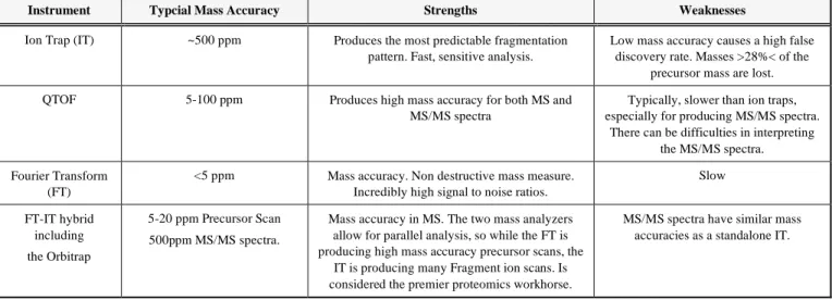
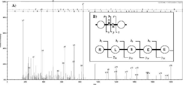
measured, which produce a fragment ion mass spectrum. In common usage, MS spectra are the precursor ion scans and MS/MS spectra are the fragment ion spectra. This workflow is often referred to as LC-MS/MS, or more generally as tandem mass spectrometry. Each MS/MS spectrum is typically associated with several important pieces of information used for final interpretation: the elution time of the precursor, the apparent mass of the precursor, the charge state of the precursor, the intensity of the precursor. The properties of this information are largely dependent on the instrumentation, how it is set up, the source of the sample, etc. There are many types of mass spectrometers used for proteomics studies and they can be broken into two artificial classes: high mass accuracy, such as QTOF and Fourier Transform instruments and low mass accuracy, such as ion trap or triple quadruple instruments. (see Table 1 for more information on specific types of mass spectrometer). It is even common to find instruments that produce high mass accuracy precursor spectra and low mass accuracy fragment ion spectra. Even the best mass spectrometers produce an imperfect dataset that contains both extraneous data and missing data. Additionally, there is always an error in the mass measurements, which can be expressed as a discrete error, 0.1 Da for example, or as a being relative term. The most common relative error term is part per million (ppm), which is very similar to percentage, except that ppm is normalized to 106 rather than 100. For example, a peptide with an m/z of 1000 and a 0.1 Da error would have a relative error of 0.01% or 100 ppm. These problems are rarely encountered in other bioinformatics workflows and account for some of the complexity in analyzing proteomics data. The fragmentation of peptides in mass spectrometers has a well defined, but somewhat complicated, nomenclature [8]. A simplified diagram is shown in Fig. (1A), where the various types of backbone fragmentation are shown. In most cases, ladder ions form, in which the fragment ion extends from either the N-terminus of the peptide (a, b, and c ions) or from the C-terminus of the peptide (x, y, and z ions). However, sometimes internal fragment ions occur when the peptide backbone fragments in more than one place. For example, immonium ions are a special class of internal ions that are generated by a- and y- type fragmentation. Fragmentation of tryptic peptides by collision induced dissociation (CID) produces an information rich data stream with at least 5 detectable types, or series, of ions: b-ions, y-ions, a-y-ions, and internal fragment ions (Fig. 1) [9]. The specific ion types generated is a function of the particular mass spectrometer being used. For example, immonium ions and internal ions are rarely seen in ion trap mass spectrometers [9]. Depending on the amino acid content of the peptide, neutral losses of water and ammonia also commonly appear in the spectra, but the final interpretation of spectra is usually dependent on the b- and y-ion series [4, 10]. Fig. (1) also shows a few simple regularities that exist between the peaks of an MS/MS spectrum. Importantly, the ion series come in complementary pairs, for example b- and y- ions form from fragmentation of the same bond and sum up to the precursor mass +1. Similarly, successive ions in the same series will be separated by the mass of an amino acid, in the case of Fig. (1A) the mass difference between b2 and b3 is the mass of Methionine. The mass differences of these
neighboring peaks, often called amino acid neighbors, can be easily calculated: k i i b aa mass b+1 = _ ; k i i y aa mass y+1 = _ (1)
where bi and yi are the masses of the of the two ion series,
and aa_massk is the mass of one of the 20 amino acid residue
ions or one of its derivatives, obtained by post-translational modification. The masses of the complementary ion series can also be calculated because they add up to MH+ +1, the mass of the precursor ion corresponding:
1 + = + ni n i y P b ; 1 + = + ni n i b P y (2) where n is the number of residues in the peptide (in Fig. 1, n=5). Substituting (2) into (1) we get
k n i n i y P aa mass b+1+ 1= _ ; k n i n i b P aa mass y+1+ 1= _ (3) Equations 1-3 are written for singly ionized species but can be extended to multiple ionization states (for example by applying equation 6). An ideal set of fragments, such as shown in Fig. (1), is sufficient to delineate the sequence of a peptide by de novo sequencing which is outside the scope of this article. Here we are concerned with using MS/MS spectra for identification of peptides, where the experimental spectra are compared to theoretical spectra derived from a protein sequence database (Fig. 1B). For this purpose, the spectra do not need to be perfect, just sufficiently free of peaks that would interfere with peptide identification. This spectral comparison approach, which is somewhat simplistically referred to as database searching, is computationally simpler and more robust than de novo sequencing or quantitative analysis.
3. SIGNAL AND NOISE
The mass spectrum is considered a histogram where the y value is proportional to the quantity of detected ions, and the x value is proportional to mass/charge ratio (m/z) of the ion (Fig. 1B). In theory, an observed spectrum F(t), can be decomposed into baseline B(t), true signal S(t) and noise e(t) components, as shown in equation (4),
) ( ) ( ) ( ) (t Bt N S t et F = + + (4) where N is a normalization factor. The true signal can be modeled as a sum of individual peaks corresponding to various molecular species present in the sample and their fragments that form within the mass spectrometer. In current MS devices the peaks of S(t) are typically narrow and their width at half height (FWHM), defines the resolution of the instrument, and can also be used to determine the uncertainty of the measurement. FWHM P resolution= n or Mass P resolution n = (5)
The noise in a raw spectrum comes from various sources: electronic noise within the detector, chemical noise coming from contaminations (matrix molecules, molecular contaminants of the sample such as ingredients of buffers, solvents, etc.) [11, 12]. Although technically incorrect, in practice, anything that is not interpretable by the automated software is often labeled as noise. For example, in Fig. (1B) all the unlabeled peaks would be considered noise, even though some of these peaks may be coming from unanticipated fragmentation pathways. The goal of signal preprocessing is to convert a spectrum into a set of peaks that are subjected to further analysis. This step is also called low-level signal processing (Fig. 2). Since noise peaks can have roughly the same shape as true peaks, only some of the noise peaks are discarded as noise in this step. But even if all the noise were perfectly discarded, the remaining spectrum will still contain extraneous peaks. This has two main reasons: i) The isotope distribution of the sample will result in a series of isotope peaks that need to be recognized and discarded in a process called deisotoping, ii) in addition an ion may exhibit more than one charge state, so singly (z=1), doubly (z=2), and triply (z=3) ionized peaks will appear in the spectrum for what is essentially a single fragment. These are recognized by a process called charge-state deconvolution. Neither i) nor ii) are noise from the measurement’s point of view, but they cause complications when interpreting the data, this is why deisotoping and deconvolution are included in many current data preprocessing schemes. After these steps, the spectra are supposed to contain only true monoisotopic and singly ionized peaks. Even after these steps, there are additional problems: a) Some peaks may correspond to chemical contaminants or irregular fragmentation events – these need to be discarded by higher order peak-filtering. b) Some of the spectra may not contain sufficient material or contain a mixture of peptides or contaminants, rather than fragments from a single peptide. These spectra are eliminated by spectrum filtering. The entire process can be viewed as applying a series of models or filters in successive steps (Table 2). At each step we can define signal and noise at a different level. In the following parts we go through the various steps of this process.
4. SIGNAL PREPROCESSING
Before low level signal processing two steps must be carried out: calibration and coarse peak detection. A calibration step maps the observed electronic signals to the inferred mass to charge ratio. This is carried out by mass standards, such as synthetic peptides which are used either as external or internal standards. In this step, the x axis of the spectrum is transformed, often by a nonlinear transformation. The conversion formulas are determined with the help of reference ions [13, 14], often by a fitting procedure [15]. For singly charged ions <4,000 Da, peptide masses can be calibrated even without reference ions, based on the observation that m/z values are concentrated in narrow ranges separated by 1.000045 Da [16]. The resulting m/z errors can be usually quite low (10 ppm for Fourier transform instruments). In LC-MS/MS experiments the intensity values (y-axis) are often expressed on a relative scale as accurate quantification of raw intensity is usually not required [17].Coarse peak detection is location of maxima in terms of m/z values. The simplest way of doing this is to pick the maximum of the peaks. A more accurate method is to take a portion of the top most intensive values and calculate their centers, this is why this step is often referred to as centroiding (Fig. 2). Importantly during the coarse peak detection the centroiding step may or may not result in a data reduction (see below for more details). In addition to simple heuristics there are a number of more advanced transforms, such as wavelet transforms [18, 19], Bayesian peak detection [20] or Gabor filters [21, 22] that can extract peaks from raw spectra with minimal parameterization. These techniques belong to a broad group of signal processing algorithms that are used within the engineering community. They offer advantages for handling large groups of spectra, but the lack of common parameters applicable to all spectra remains a fundamental problem left to the experimenter. Current mass spectrometers often contain software that takes care of many of these steps and is often done automatically during data collection and remains somewhat hidden from the experimenter. In addition, most methodologies combine several steps.
Table 1. Major Types of Instruments
Instrument Typcial Mass Accuracy Strengths Weaknesses
Ion Trap (IT) ~500 ppm Produces the most predictable fragmentation pattern. Fast, sensitive analysis.
Low mass accuracy causes a high false discovery rate. Masses >28%< of the
precursor mass are lost. QTOF 5-100 ppm Produces high mass accuracy for both MS and
MS/MS spectra
Typically, slower than ion traps, especially for producing MS/MS spectra.
There can be difficulties in interpreting the MS/MS spectra. Fourier Transform
(FT)
<5 ppm Mass accuracy. Non destructive mass measure. Incredibly high signal to noise ratios.
Slow FT-IT hybrid including the Orbitrap 5-20 ppm Precursor Scan 500ppm MS/MS spectra.
Mass accuracy in MS. The two mass analyzers allow for parallel analysis, so while the FT is producing high mass accuracy precursor scans, the
IT is producing many Fragment ion scans. Is considered the premier proteomics workhorse.
MS/MS spectra have similar mass accuracies as a standalone IT.
5. SPECTRUM PROCESSING
A MS/MS spectrum often contains multiple forms of the exact same peptide fragment. These different forms may arise either because the peptide has more than one stable charge state (charge clusters) or because the peptide contains several heavy isotopes of its elemental composition. For biological samples, these isotopic clusters, or envelopes, are dominated by the stable isotopes of Carbon. The calibration and coarse peak calling steps are required before these additional problems can be corrected. The goal of the next steps of preprocessing is to obtain a MS/MS spectrum in which each ion is represented by a single peak, so the clusters must be identified and replaced by a single peak.
Charge State Deconvolution
It is common for a peptide (or fragment) to have more than one charge state. These multiple charge states make the
MS/MS spectrum difficult to interpret and the additional charge states add little valuable information. For example, it is not uncommon to find a single peptide existing as a +1, a +2 and a +3 ion. This results in three distinct peaks appearing and the observed m/z follows this relationship:
z
H z z
m/ = MolecularWeight+ * (6) where z is the number of charges and H is the mass of a proton. For example a peptide with a molecular weight of 1000, would have a m/z of 1001 for z=1, 501 for z=2, and 334.33 for z = 3. It is common practice to report the singly charged mass (MH+), even when multiply charged ions are measured. The process of deconvolution involves identifying peaks that arise from these multiple charge states. Once such a cluster is identified, the intensities are summed to the most intense peak and the rest of the cluster members get
Fig. (1). Anatomy of a peptide MS/MS spectrum. A) Example of a spectrum that has been matched to peptide sequence RLSEETTEFSLGGIFLK. For example b3 and y14 sum to the precursor mass. B) Simplified fragmentation pattern of a peptide. In the mass
spectrometer, a peptide breaks into two parts at various points of the peptide backbone (top). Of these, the N-terminal b- and C-terminal y-ions (bottom) carry most of the information.
Table 2. Steps of Data Preprocessing in MS-Based Proteomics.
Levels of preprocessing Operation Signal Noise
1 Detector signal Signal preprocessing Calibration
Coarse peak dentification
Peak (shape) Baseline
2 Peak cluster level Spectrum processing
Charge state deconvolution, Deisotoping
Peak clusters with correct structure (united into single peaks)
No clusters, bad periodicities etc.
3 Spectrum level Data filtering Peak filtering, Spectrum filtering
Peak (correct intensity, spatial distribution)
Noise peaks, noise spectra
removed. Charge clusters are typically problematic for MS/MS spectra only when the charge state of the precursor ion is greater than 3. For tryptic fragments, this is a fairly uncommon event and charge state deconvolution is frequently skipped.
Deisotoping or Monoisotoping
Attempts to simplify the cluster of ions – sometimes called isotopic envelopes - that forms because of the naturally occurring heavy isotopes (Fig. 3). For example, the element Carbon contains 6 protons and 6 neutrons, giving it a mass of ~12 Da. However about 1% of the Carbon has 7 neutrons, which makes it a slightly heavier ~13 Da. For the average sized peptide with 50 Carbon atoms, this results in the monoisotopic peak, which contains only light atoms being about 50% of the total, the +1 13C peak is ~30% of the total, and the +2 13C is 13% of the total and so on. Typically 3 to 6 isotopic peaks are detectable with modern day instruments and the specific ratios between the peaks depends on the size of the peptide, as the greater the number of Carbons in a peptide, the more likely you are to find a heavy isotope of Carbon. Unlike the multiple charge states, the isotope peaks can be highly informative and can give clues to the elemental composition and whether or not it is a true peak or a noise peak [23]. In fact, the isotope pattern can also reveal the charge state of the peak and is often used for this purpose [24]. Using our previous example of the 1000 molecular weight peptide, with z=1 the isotopic peaks will be spaced every 1 Da (the mass of the neutron / 1), with z=2 the isotopic peaks will be spaced every 0.5 Da (the mass of the neutron/ 2), and with z=3 the isotopic peaks will be spaced every 0.3 Da (the mass of the neutron / 3). Therefore, this isotopic spacing is an efficient means of deconvoluting spectra and converting all m/z values to the +1 charge state. Since there is extra information in the isotopic pattern, charge state deconvolution is usually applied before deisotoping. In the process of deisotoping, the series of an isotopic envelope are identified, removed from the spectrum and replaced by the monoisotopic peak. The intensity either remains unchanged, or, more commonly, the intensity is transformed by summing the intensity of all the peaks in the isotope envelope.
Even though the intensity distribution and the m/z distribution of the clusters can be reliably calculated, problems arise if isotopic clusters and/or charge clusters
overlap with each other. Deconvolution of overlapping clusters is especially complicated when a spectrum is derived from more than one peptide, for detailed discussion on this subject see Bern et al. 2010 [25]. One of the major goals of these steps is data reduction. The data reduction can be quite dramatic, with full profile spectra typically being 10-200 times larger than their centroided derivatives. At this point in the workflow, relatively simple strategies have been used for data reduction and the result should be a reliable list of peaks that can be used for more complex algorithms.
6. DATA FILTERING STRATEGIES
There are two strategies for producing high quality spectra: i) Peak filtering and ii) Spectrum filtering. i) Peak filtering approaches identify unwanted peaks, including
Fig. (2). Conversion of a profile spectrum into peaks (peak centroiding). The centroided values are picked either as the maximum of the peak, or an intensity-weighted average of the values above the half maximum intensity (inset). Note that the profile data (top) are retained after the peaks have been identified.
Fig. (3). Charge clusters and isotope clusters of a single peptide fragment.
noise peaks, and remove them from the spectra. Noise peaks are identified either by their low intensities or by the fact that they do not obey the fragmentation rules (eqn. 1-3). The fundamental goal is to increase the reliability of database searching as well as to save storage space (data compression) ii) Spectrum filtering approaches, on the other hand, try to identify low quality spectra by their peculiar intensity or m/z distributions and excluding them from further analysis. The two approaches are not necessarily mutually exclusive.
Peak Filtering
Noise peaks can have shapes that are similar to true peaks, which make them difficult to identify using simple classification schemes. One relatively reliable approach is to differentiate based on intensity. This case is driven by the assumption that true peaks (or signal) tend to be of higher intensity than unwanted (noise peaks) [26]. This often leads to problems, as peptides do not fragment uniformly along their backbone and can result in high intensity peaks clustering with in a spectrum [3]. Renard and associates distinguished various simple intensity filters [3]:
“Intensity thresholding” only peaks above a certain intensity threshold are retained, the threshold can be defined as a percentage (typically ~5%) of the highest intensity [4]. “Top X intensity” filters sort all ions by decreasing intensity and keep the first n ions [26, 27]. The top 60 to 100 peaks gives good results for many datasets, even though small peptides may have less that 100 peaks, while big peptides have many more than that. However one can also note that a peptide cannot have more b,y,a and immonium ions than 4 times the number of its amino acids, so in principle one can define X as a function of the molecular precursor mass of the peptides
8 . 120 + =kMH X (7)
where MH+ is the precursor mass, 120.8 is the approximate mass of the average amino acid and k is a scaling factor. “Top X in Y regions” filters aim to alleviate the problem that high intensity peaks may cluster in certain parts of the spectrum. In this case the spectrum is divided into Y equal regions (defined with a certain overlap), and the top X intensities are retained in each of the regions [3].
“Top X intensity in a window of +/- Z” approaches, first sort the peaks by decreasing intensity, then, starting with the highest intensity peak, retain the top X intensities in a window of +/- Z m/z right and left from the most intensive peak and exclude all other peaks. This is repeated until all peaks are selected or rejected [4, 28]. The Z is usually set to be smaller than the mass of an amino acid, because there should not be many true peaks with spacing less than that of an amino acid and X is usually set to 1 or 2 to account for ions from two different ion series occurring in the same small window [4].
A more sophisticated algorithm, THRASH, estimates the signal to noise ratio for each peak within a window of +/- Z (Z ~25 Da), using a histogram of frequency vs. intensity within the window [29]. The noise is calculated by the full width at half maximum (FWHM) of the smooth histogram,
as the most frequent intensity value within the window, Ib is
used as background intensity, so for a peak of Ip intensity,
the signal to noise ratio is calculated as
FWHM I I N
S/ = p b (8) and peaks above a threshold level are accepted, repeating the selection of overlapping windows along the spectrum.
In addition to these simple assumptions, one can use the fragmentation rules or other chemical rules to select peaks that are not likely to be noise. Bern (2007) used peaks obeying eq (1) to identify high quality spectra [30]. Ning and Leong used the same rule for adding pseudo-peaks (peaks originally not present in the spectrum) in order to increase the performance of peptide sequencing [31]. Reiz and associates designed a peak-filter that only retains peaks that obey at least one of equations (1-3) [32].
Spectrum Filtering
The goal of spectrum filtering is to distinguish high and low quality spectra. The goal is either to exclude low quality spectra from further analysis by database searching (pre-filtering), or to find potential high quality spectra in a set discarded by database searching, and to submit them to a second round of database search (post-filtering).
Low quality spectra (Fig. 4) are typically either i) noise spectra that are either of too low intensity or do not contain sufficient peptide peaks (in number or in intensity); or ii) contaminated spectra that contain high amounts of certain common contaminants (polymers, protein contaminants); or iii) spectra that contain a mixture of peptides that would hamper peptide identification by database search. Noise spectra have a relatively uniform intensity distribution, with no obvious amino acid spacing between the peaks, and the isotope distributions are different from that of peptides. Mixture spectra contain too many high intensity peaks that have the characteristic isotopic distribution of peptides, but many of the high intensity peaks are closer to each other than the molecular weight of an amino acid. In principle, some of these problems would require different approaches. Same as with peak filtering, quality control of spectra relies on the analysis of the intensity distributions and the m/z distribution of the peaks and may also include specific treatment of amino acid, isotope and/or charge series. The resulting algorithms are quite diverse in scope, and in addition to simple chemical heuristics it is customary to determine some of the decision parameters by learning from datasets of high and low quality spectra.
Bern et al (2004) used several handcrafted features of varying sophistication (number of peaks, identities, number of possible amino acid pairs and b-pairs within a certain tolerance, etc.) to train Quadratic Discriminate Analysis (QDA) classifiers on datasets in which spectra identified by the SEQUEST algorithm were denoted good, all others as bad [33]. The best classifier combination could identify 75% of the unidentifiable spectra while discarding only 10% of the identifiable spectra.
Xu and associates used parameters related either to peak intensity (number of peaks above adjustable thresholds of peak intensity, % total ion current, etc.) or to peak spacing
(average distances between peaks in various intensity ranges) to construct a QDA discriminant function parameterized on manually validated datasets [34]. The resulting classifier was able to recover many high quality spectra unassigned by commercial search engines.
Flikka and associates used a straightforward learning approach based on 17 general spectrum parameters (including the number of peaks, peaks over 0.1 relative intensity, no of significant peaks divided by precursor mass, etc.) that were combined to build a committee of classifiers trained on datasets in which spectra identified by the MASCOT algorithm were denoted high quality, all others as low quality [35]. It was found that a trained classifier could identify half of the unidentified spectra as bad, and many of the unidentified peptides predicted as high quality could be confirmed as correct hits.
Nesvizhskii and associates designed a learning algorithm that is based on 40 spectrum features [36]. Part of these are general spectrum parameters, another part is related to short amino acid reads, and another part of them are related to the number of b- ions, y- ions and b-y pairs that correspond to the charge state of the precursor. The quality scores computed for individual features are combined into a linear discriminant function which is parameterized on datasets of good and bad spectra, pre-labeled by MASCOT analysis. Hoopman and associates built a sophisticated preprocessing algorithm, Hardklör, that is based on the analysis of Peptide Isotope Distribution (PIDs) in 5 distinct steps [23]: 1) A THRASH-style peak finding [29], 2) Charge state estimation, 3) Averagine
Modeling and Monoisotopic Mass prediction [37]; 4) Unusual PID detection and 5) Analysis. The Averagine model of McLafferty and associates [37] uses the weighted average of the elemental composition of amino acids found in proteins for estimating the PID of a polypeptide and deviations above a certain threshold are considered as unusual. The accepted PIDs are then compared to observed data in a combinatorial fashion and combinations that exceed
a certain similarity threshold are accepted. This process allows recovery of a large portion of unidentified spectra, the authors estimated that over 11% of the MS-MS spectra in their dataset were composed of fragment ions from multiple molecular species.
7. SPECTRUM CLUSTERING
Clustering of spectra is a logical step since the spectrum of a peptide may be taken several, sometimes many times during the same experiment so joining (summing or averaging) nearly identical spectra can increase accuracy and save storage memory at the same time. The advantages and pitfalls of clustering proteomics data are not dissimilar to those seen in other fields. Several groups developed clustering methods capable of handling large spectrum datasets [38-43] and the individual strategies differ in many fine details, regarding how the clusters are represented, when new members are allowed to join etc. All these details will influence the sensitivity of protein identification since low quality spectra that often represent the most interesting biological objects, may be misclassified and/or eliminated by mistake. On the other hand, clustering of spectra has specific benefits as it can help one to recognize and eliminate known protein/peptide contaminants, or highlight non-peptide contaminants such as polymers with characteristic, non-peptidic periodicities in their spectra. Common-sense grouping scenarios were included in the earliest work, for instance Yates and associates grouped spectra based on the precursor mass and chromatographic elution time [44]. This method merges MS/MS spectra from the same liquid chromatography peak. Furthermore, spectra of post-translationally modified (PTM) and unmodified versions of the same fragment can be clustered together, which helps one to detect PTMs [40, 45]. However, this typically requires a more sophisticated algorithm as the modified and unmodified peptides rarely have the same chromatographic elution time [40, 45].
8. PROGRAMS
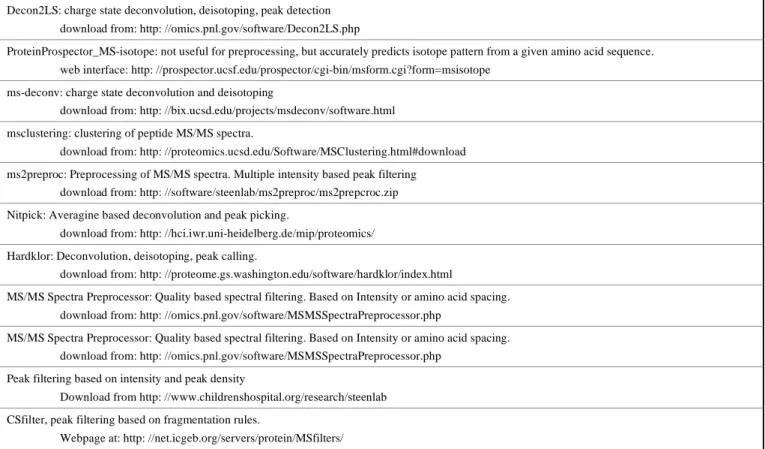
Most laboratories make use of the platform-specific and proprietary preprocessing programs provided by the instrument manufacturers. Some of the publicly available programs are listed in Table 3. The publicly available R/Bioconductor program package and MATLAB contain tools for processing mass spectra.
9. CONCLUSIONS AND PERSPECTIVES
A typical proteomics experiment produces a large, information-rich data stream. The workflow produces a large amount of extraneous data that can hamper the final analysis. This extra data takes the form of redundant peaks, such as multiple charge states, chemical and detector noise, unanticipated peaks and isotope clusters. The raw data is rarely used directly and is subject to several signal processing steps. The overall goal of signal processing is to remove these redundant peaks, such as multiple charge states, chemical and detector noise, unanticipated peaks and isotope clusters. The raw data is rarely used directly and is subject to several signal processing steps. This removal results not only in more efficient analysis, but also aids in the storage and transfer of data between analysis programs.
Fig. (4). Typical MS/MS spectra after charge deconvolution and deisotoping. The inset is the frequency distribution of the spectra.
Before, even rudimentary, signal processing can begin the spectrum is usually calibrated and a coarse peak calling is performed. The coarse peak calling will determine the features that signal processing algorithms will consider and the calibration ensures that the algorithms will use the highest accuracy data obtainable.
The signal processing algorithms discussed here are based on two fundamental kinds of descriptions of mass spectra: unstructured and structured. Unstructured descriptions typically use aggregate variables of the spectrum, such as the number of peaks, average or maximum intensities, distributions, etc., and employ general computational approaches also used in other fields such as optical or acoustic signal processing. Methods using unstructured descriptors are simple to understand and to implement, and the algorithms are often very fast. However the parameterization is usually not universal, for instance there are no general intensity thresholds, etc. As a result, the unstructured classifiers typically have to be adjusted in such a way that there is a balance between retaining unwanted peaks and discarding valuable peaks. On the other hand, structured descriptions use discrete variables, such as inter-peak relationships such as those that correlate with amino acid masses, isotope distributions, or other behaviors consistent with peptide sequence, and the computational approaches based on them are specific to proteomics. Once structure is introduced into the classifiers (even at such a modest level as Fourier transformation of the signals) the efficiency of the classifier increases. However, the principles of structured classifiers are often more difficult to implement.
The current development of instrumentation is geared towards faster and faster data acquisition. An instrument with fast data acquisition is ideal for the bottom up work flow, as these instruments will perform more analyses on the sample than slower instruments. There is another trend to move towards the analysis of intact proteins without enzyme digestion, the so called top down workflow. Although the top down workflow will result in simpler samples, which will generate fewer spectra, the protein spectra are more complex than peptide spectra. Therefore, there is a growing need for computational methods that can efficiently process peptide and protein based spectra. These will undoubtedly be a mixture of signal processing algorithms borrowed from other fields and algorithms designed specifically for features found in peptide or protein spectra.
CONFLICT OF INTEREST
None declared.
ACKNOWLEDGEMENT
None declared.
REFERENCES
[1] Aebersold R, Mann M. Mass spectrometry-based proteomics. Nature 2003; 422(6928): 198-207.
[2] Webb-Robertson BJ, Cannon WR. Current trends in computational inference from mass spectrometry-based proteomics. Briefings in bioinformatics. 2007; 8(5): 304-17.
[3] Renard BY, Kirchner M, Monigatti F, et al. When less can yield more - Computational preprocessing of MS/MS spectra for peptide identification. Proteomics 2009; 9(21): 4978-84.
[4] Geer LY, Markey SP, Kowalak JA, et al. Open mass spectrometry search algorithm. J Proteome Res. 2004; 3(5): 958-64.
Table 3. Non-Commercial, Publicly Accessible Programs for Preprocessing Mass Spectra.
Decon2LS: charge state deconvolution, deisotoping, peak detection download from: http: //omics.pnl.gov/software/Decon2LS.php
ProteinProspector_MS-isotope: not useful for preprocessing, but accurately predicts isotope pattern from a given amino acid sequence. web interface: http: //prospector.ucsf.edu/prospector/cgi-bin/msform.cgi?form=msisotope
ms-deconv: charge state deconvolution and deisotoping
download from: http: //bix.ucsd.edu/projects/msdeconv/software.html msclustering: clustering of peptide MS/MS spectra.
download from: http: //proteomics.ucsd.edu/Software/MSClustering.html#download ms2preproc: Preprocessing of MS/MS spectra. Multiple intensity based peak filtering
download from: http: //software/steenlab/ms2preproc/ms2prepcroc.zip Nitpick: Averagine based deconvolution and peak picking.
download from: http: //hci.iwr.uni-heidelberg.de/mip/proteomics/ Hardklor: Deconvolution, deisotoping, peak calling.
download from: http: //proteome.gs.washington.edu/software/hardklor/index.html
MS/MS Spectra Preprocessor: Quality based spectral filtering. Based on Intensity or amino acid spacing. download from: http: //omics.pnl.gov/software/MSMSSpectraPreprocessor.php
MS/MS Spectra Preprocessor: Quality based spectral filtering. Based on Intensity or amino acid spacing. download from: http: //omics.pnl.gov/software/MSMSSpectraPreprocessor.php
Peak filtering based on intensity and peak density
Download from http: //www.childrenshospital.org/research/steenlab CSfilter, peak filtering based on fragmentation rules.
[5] McHugh L, Arthur JW. Computational methods for protein identification from mass spectrometry data. PLoS Comput Biol 2008; 4(2): e12.
[6] Nesvizhskii AI. A survey of computational methods and error rate estimation procedures for peptide and protein identification in shotgun proteomics. J Proteomics 2010; 73(11): 2092-123. [7] Nesvizhskii AI. Protein identification by tandem mass spectrometry
and sequence database searching. Methods Mol Biol 2007; 367: 87-119.
[8] Roepstorff P, Fohlman J. Proposal for a common nomenclature for sequence ions in mass spectra of peptides. Biomed Mass Spectrom 1984; 11(11): 601.
[9] Mitchell Wells J, McLuckey SA, Burlingame AL. Collision Induced Dissociation (CID) of Peptides and Proteins. Methods Enzymol Academic Press 2005: 148-85.
[10] Craig R, Beavis RC. Tandem: matching proteins with tandem mass spectra. Bioinformatics 2004; 20: 1466-7.
[11] Hu J, Coombes KR, Morris JS, Baggerly KA. The importance of experimental design in proteomic mass spectrometry experiments: some cautionary tales. Brief Funct Genomic Proteomic 2005; 3(4): 322-31.
[12] Baggerly KA, Morris JS, Wang J, Gold D, Xiao LC, Coombes KR. A comprehensive approach to the analysis of matrix-assisted laser desorption/ionization-time of flight proteomics spectra from serum samples. Proteomics 2003; 3(9): 1667-72.
[13] Vestal M, Juhash P. Resolution and mass accuracy in matrix-assisted laser desorption ionization time-of-flight. J Am Soci Mass Spectrom 1998; 9: 892-911.
[14] Christian NP, Arnold RJ, Reilly JP. Improved calibration of time-of-flight mass spectra by simplex optimization of electrostatic ion calculations. Anal Chem 2000; 72(14): 3327-37.
[15] Hack CA, Benner WH. A simple algorithm improves mass accuracy to 50-100 ppm for delayed extraction linear matrix-assisted laser desorption/ionization time-of-flight mass spectrometry. Rapid Commun Mass Spectrom 2002; 16(13): 1304-12.
[16] Gay S, Binz PA, Hochstrasser DF, Appel RD. Modeling peptide mass fingerprinting data using the atomic composition of peptides. Electrophoresis 1999; 20(18): 3527-34.
[17] Zubarev R, Mann M. On the proper use of mass accuracy in proteomics. Mol Cell Proteomics 2007; 6(3): 377-81.
[18] Coombes KR, Tsavachidis S, Morris JS, Baggerly KA, Hung MC, Kuerer HM. Improved peak detection and quantification of mass spectrometry data acquired from surface-enhanced laser desorption and ionization by denoising spectra with the undecimated discrete wavelet transform. Proteomics 2005; 5(16): 4107-17.
[19] Du P, Kibbe WA, Lin SM. Improved peak detection in mass spectrum by incorporating continuous wavelet transform-based pattern matching. Bioinformatics 2006; 22(17): 2059-65.
[20] Jianqiu Z, Xiaobo Z, Honghui W, et al. Bayesian peptide peak detection for high resolution TOF mass spectrometry. IEEE Press 2010: 5883-94.
[21] Nguyen N, Huang H, Oraintara S, Vo A. GaborLocal: peak detection in mass spectrum by Gabor filters and Gaussian local maxima. Comput Syst Bioinform Conf 2008; 7: 85-96.
[22] Nguyen N, Huang H, Oraintara S, Vo A. Peak detection in mass spectrometry by Gabor filters and envelope analysis. J Bioinform Comput Biol 2009; 7(3): 547-69.
[23] Hoopmann MR, Finney GL, MacCoss MJ. High-speed data reduction, feature detection, and MS/MS spectrum quality assessment of shotgun proteomics data sets using high-resolution mass spectrometry. Anal Chem 2007; 79(15): 5620-32.
[24] Klammer AA, Wu CC, MacCoss MJ, Noble WS. Peptide charge state determination for low-resolution tandem mass spectra. Proc IEEE Comput Syst Bioinform Conf 2005: 175-85.
[25] Bern M, Finney G, Hoopmann MR, Merrihew G, Toth MJ, MacCoss MJ. Deconvolution of mixture spectra from ion-trap data-independent-acquisition tandem mass spectrometry. Anal Chem 2010; 82(3): 833-41.
[26] Hansen KC, Schmitt-Ulms G, Chalkley RJ, Hirsch J, Baldwin MA, Burlingame AL. Mass spectrometric analysis of protein mixtures at
low levels using cleavable 13C-isotope-coded affinity tag and multidimensional chromatography. Mol Cell Proteomics 2003; 2(5): 299-314.
[27] Chalkley RJ, Baker PR, Huang L, et al. Comprehensive analysis of a multidimensional liquid chromatography mass spectrometry dataset acquired on a quadrupole selecting, quadrupole collision cell, time-of-flight mass spectrometer: II. New developments in Protein Prospector allow for reliable and comprehensive automatic analysis of large datasets. Mol Cell Proteomics 2005; 4(8): 1194-204.
[28] Tanner S, Shu H, Frank A, et al. InsPecT: identification of posttranslationally modified peptides from tandem mass spectra. Anal Chem 2005; 77(14): 4626-39.
[29] Horn DM, Zubarev RA, McLafferty FW. Automated reduction and interpretation of high resolution electrospray mass spectra of large molecules. J Am Soc Mass Spectrom 2000; 11(4): 320-32. [30] Bern M, Cai Y, Goldberg D. Lookup peaks: a hybrid of de novo
sequencing and database search for protein identification by tandem mass spectrometry. Anal Chem 2007; 79(4): 1393-400. [31] Ning K, Leong HW. Algorithm for peptide sequencing by tandem
mass spectrometry based on better preprocessing and anti-symmetric computational model. Comput Syst Bioinform Conf 2007; 6: 19-30.
[32] Reiz B, Kertesz-Farkas A, Pongor S, Myers MP. Chemical rule-based filtering of MS/MS spectra. in press. 2011.
[33] Bern M, Goldberg D, McDonald WH, Yates JR, 3rd. Automatic quality assessment of peptide tandem mass spectra. Bioinformatics. 2004; 20(Suppl 1): i49-54.
[34] Xu M, Geer LY, Bryant SH, et al. Assessing data quality of peptide mass spectra obtained by quadrupole ion trap mass spectrometry. J Proteome Res 2005; 4(2): 300-5.
[35] Flikka K, Martens L, Vandekerckhove J, Gevaert K, Eidhammer I. Improving the reliability and throughput of mass spectrometry-based proteomics by spectrum quality filtering. Proteomics 2006; 6(7): 2086-94.
[36] Nesvizhskii AI, Roos FF, Grossmann J, et al. Dynamic spectrum quality assessment and iterative computational analysis of shotgun proteomic data: toward more efficient identification of post-translational modifications, sequence polymorphisms, and novel peptides. Mol Cell Proteomics 2006; 5(4): 652-70.
[37] Senko MW, Beu SC, McLafferty FW. Automated assignment of charge states from resolved isotopic peaks for multiply charged ions. J Am Soc Mass Spectrom 1995; 6(1): 52-6.
[38] Beer I, Barnea E, Ziv T, Admon A. Improving large-scale proteomics by clustering of mass spectrometry data. Proteomics 2004; 4(4): 950-60.
[39] Flikka K, Meukens J, Helsens K, et al. Implementation and application of a versatile clustering tool for tandem mass spectrometry data. Proteomics 2007; 7(18): 3245-58.
[40] Frank AM, Bandeira N, Shen Z, et al. Clustering millions of tandem mass spectra. J Proteome Res 2008; 7(1): 113-22.
[41] Gentzel M, Kocher T, Ponnusamy S, Wilm M. Preprocessing of tandem mass spectrometric data to support automatic protein identification. Proteomics 2003; 3(8): 1597-610.
[42] Tabb DL, MacCoss MJ, Wu CC, Anderson SD, Yates JR, 3rd. Similarity among tandem mass spectra from proteomic experiments: detection, significance, and utility. Anal Chem 2003; 75(10): 2470-7.
[43] Tabb DL, Thompson MR, Khalsa-Moyers G, VerBerkmoes NC, McDonald WH. MS2Grouper: group assessment and synthetic replacement of duplicate proteomic tandem mass spectra. J Am Soc Mass Spectrom 2005; 16(8): 1250-61.
[44] Yates JR, 3rd, Eng JK, McCormack AL, Schieltz D. Method to correlate tandem mass spectra of modified peptides to amino acid sequences in the protein database. Anal Chem 1995; 67(8): 1426-36.
[45] Savitski MM, Nielsen ML, Zubarev RA. ModifiComb, a new proteomic tool for mapping substoichiometric post-translational modifications, finding novel types of modifications, and fingerprinting complex protein mixtures. Mol Cell Proteomics 2006; 5(5): 935-48.