Testing for Serial Correlation, Spatial Autocorrelation and Random
E
ff
ects Using Panel Data
∗by
Badi H. Baltagi
Department of Economics, Texas A&M University, College Station, Texas 77843-4228, USA
(979) 845-7380 [email protected]
Seuck Heun Song, Byoung Cheol Jung
Department of Statistics, Korea University, Sungbuk-Ku, Seoul, 136-701, Korea
[email protected] [email protected]
and
Won Koh
Center for DM&S, Korea Institute for Defense Analyses (KIDA) Cheong Ryang P.O Box 250, Seoul, 130-650, Korea
September 2003
Keywords: Panel data, Spatial error correlation, serial correlation, Lagrange Multiplier tests, Likelihood Ratio tests.
JEL classification: C23, C12
ABSTRACT
This paper considers a spatial panel data regression model with serial correlation on each spatial unit over time as well as spatial dependence between the spatial units at each point in time. In addition, the model allows for heterogeneity across the spatial units using random effects. The paper then derives several Lagrange Multiplier tests for this panel data regression model including a joint test for serial correlation, spatial autocorrelation and random effects. These tests draw upon two strands of earlier work. The first is the LM tests for the spatial error correlation model discussed in Anselin and Bera (1998) and in the panel data context by Baltagi, Song and Koh (2003). The second is the LM tests for the error component panel data model with serial correlation derived by Baltagi and Li (1995). Hence the joint LM test derived in this paper encompasses those derived in both strands of earlier works. In fact, in the context of our general model, the earlier LM tests become marginal LM tests that ignore either serial correlation over time or spatial error correlation. The paper then derives conditional LM and LR tests that do not ignore these correlations and contrast them with their marginal LM and LR counterparts. The small sample performance of these tests is investigated using Monte Carlo experiments. As expected, ignoring any correlation when it is significant can lead to misleading inference.
1
Introduction
Spatial models deal with correlation across spatial units usually in a cross-section setting, see Anselin (1988). Panel data models allow the researcher to control for heterogeneity across these units, see Baltagi (2001). Spatial panel models can control for both hetero-geneity and spatial correlation, see Baltagi, Song and Koh (2003). Recent spatial panel data applications in economics include household level survey data from villages observed over time to study nutrition, see Case (1991); per-capita expenditures on police to study their effect on reducing crime across counties, see Kelejian and Robinson (1992); the pro-ductivity of public capital like roads and highways in the private sector across U.S. states, see Holtz-Eakin (1994); hedonic housing equations using residential sales, see Bell and Bockstael (2000); unemployment clustering with respect to different social and economic metrics, see Conley and Topa (2002); and spatial price competition in the wholesale gaso-line markets, see Pinkse, Slade and Brett (2002). This paper adds another dimension to the correlation in the error structure. Namely, serial correlation in the remainder error term. The spatial error component model assumes that the only correlation over time is due to the presence of the same region effect across the panel. This may be a restric-tive assumption in the analysis of panel data, such as investment across regions, where an unobserved shock in this period will affect the behavioral relationship for at least the next few periods. Ignoring the serial correlation in the error results in consistent, but inefficient estimates of the regression coefficients and biased standards errors, see Baltagi (2001). This paper considers a spatial panel data regression model with serial correlation on each spatial unit over time as well as spatial dependence between the spatial units at each point in time.
For the panel data model with no spatial effects, Baltagi and Li (1995) addressed the problem of jointly testing for serial correlation and individual effects. Testing for spatial dependence has been extensively studied by Anselin (1988, 1999) and Anselin and Bera (1998), to mention a few. Baltagi, Song and Koh (2003) considered the problem of jointly testing for random region effects in the panel as well as spatial correlation across these regions. However, the last study did not consider the added problem of serial correlation in the remainder error term. This paper generalizes the previous studies by deriving test statistics for the spatial panel data model with serial correlation. In particular, this paper derives joint and conditional LM and LR tests and studies their small sample properties using Monte Carlo experiments. One directional tests that test for spatial error correlation, for e.g., ignoring the presence of serial correlation over time and random effects among the spatial units could yield misleading inference when one or both of the left out components are significant. Conditional LM tests are proposed and their performance is contrasted with the corresponding marginal counterparts. Our Monte Carlo results show that these conditional tests guard against possible misspecification.
2
The Model
Consider the following panel data regression model
where yti is the observation on the ith region for the the tth time period, Xti denotes
the kx1 vector of observations on the nonstochastic regressors and uti is the regression
disturbance. In vector form, the disturbance vector of (2.1) is assumed to have random re-gion effects, spatially autocorrelated residual disturbances and afirst order autoregressive remainder disturbance term:
ut=µ+²t, (2.2)
with
²t=λW ²t+νt, and νt=ρνt−1+et (2.3)
whereu0t= (ut1, ..., utN)and²t,νtandetare similarly defined. µ0 = (µ1, µ2, .., µN)denote
the vector of random region effects which are assumed to be IIN(0,σ2
µ). λ is the scalar
spatial autoregressive coefficient with |λ| < 1, whileρ is the time-wise serial correlation coefficient satisfying |ρ|<1. W is a known N×N spatial weight matrix whose diagonal elements are zero. W also satisfies the condition that IN −λW is nonsingular, whereIN
is an identity matrix of dimension N. eti∼IIN(0,σ2e) and νi,0 ∼N(0,σ2e/(1−ρ2)). We
assume thatµand ²are independent. One can rewrite (2.3) as
²t= (IN −λW)−1νt=B−1νt (2.4)
whereB=IN−λW. The model (2.1) can be rewritten in matrix notation as
y=Xβ+u (2.5)
whereyis of dimensionN T×1,X isN T×k,β isk×1and uis aN T×1. X is assumed to be of full column rank and its elements are assumed to be bounded in absolute value. The disturbance term can be written in vector form as
u= (ιT ⊗IN)µ+ (IT ⊗B−1)ν (2.6)
where ν0 = (ν0
1,ν02, ..,ν0T) and u is similarly defined. ιT is a vector of ones of dimension
T,IT is an identity matrix of dimensionT and ⊗denotes the Kronecker product. Under
these assumptions, the variance-covariance matrix of ucan be written as
Ω=σ2µ(JT ⊗IN) + (V ⊗(B0B)−1) (2.7)
where JT is a matrix of ones of dimension T, and V is the familiar AR(1)
variance-covariance matrix of dimensionT, V =E(νν0) =σ2e µ 1 1−ρ2 ¶ V1 =σ2eVρ (2.8) where V1 = 1 ρ ρ2 · · · ρT−1 ρ 1 ρ · · · ρT−2 .. . ... ... . .. ... ρT−1 ρT−2 ρT−3 · · · 1 and Vρ= µ 1 1−ρ2 ¶ V1.
It is well established that the Prais-Winsten transformation C= (1−ρ2)1/2 0 0 · · · 0 0 0 −ρ 1 0 · · · 0 0 0 .. . ... ... ... ... . .. ... 0 0 0 · · · −ρ 1 0 0 0 0 · · · 0 −ρ 1 (2.9)
transforms the usual AR(1) model into serially uncorrelated classical disturbances with CV C0 = σ2eIT. For panel data, this C transformation has to be applied repeatedly for
N individuals. From (2.5), the transformed spatial panel data regression disturbances are given by: u∗ = (C⊗IN)u= (CιT ⊗IN)µ+ (C⊗B−1)ν = (1−ρ)(ιαT ⊗IN)µ+ (C⊗B−1)ν (2.10) whereCιT = (1−ρ)ιαT with ιαT = (α,ι 0 T−1) and α= q 1+ρ 1−ρ.
Therefore, the variance-covariance matrix of the Prais-Winsten transformed spatial panel data model is given by
Ω∗=E(u∗u∗0) = (1−ρ)2σ2µ(ιαTιαT0⊗IN) +σ2e(IT ⊗(B0B)−1) (2.11)
since (C⊗B−1)E(νν0)(C⊗B−1)0 =σ2e(IT ⊗(B0B)−1). Replace ιαTιαT0 by its idempotent
counterpart d2J¯Tα, where J¯Tα = ιαTιαT0/d2 and d2 = ιαT0ιαT = α2 + (T −1). Replace IT by
Eα
T + ¯JTα, whereETα=IT −J¯Tα and collect like terms, see Baltagi and Li (1995), we get
Ω∗= ¯JTα⊗[d2(1−ρ)2σ2µIN +σ2e(B0B)−1] +EαT ⊗[σ2e(B0B)−1] (2.12)
One can easily verify that
Ω∗−1= ¯JTα⊗Z+ETα⊗[(σ2e)−1(B0B)] (2.13) whereZ = [d2(1−ρ)2σ2
µIN+σ2e(B0B)−1]−1.
Note that|Ω∗|=|d2(1−ρ)2σ2µIN+σ2e(B0B)−1||σ2e(B0B)−1|(T−1), see Magnus (1982). Also,
Ωin (2.7) is related toΩ∗ in (2.11) byΩ∗ = (C⊗IN)Ω(C0⊗IN)with|C|=
p
1−ρ2 and
|IN ⊗C|=|C|N. Under the assumption of normality, the log-likelihood function for this
model can be written as:
L(β,σ2e,ρ,λ) = Const+1 2Nln(1−ρ 2) −1 2ln|d 2(1 −ρ)2σ2µIN +σ2e(B0B)−1| −N(T2−1)ln(σe2) + (T−1) ln|B|−1 2u ∗0Ω∗−1 u∗ (2.14) whereu∗ is given by (2.10) andΩ∗−1 is given by (2.13).
3
Test Statistics
The hypotheses under the consideration in this model are the following:
(J) H0a: λ = ρ = σ2µ = 0, this is the joint hypothesis that there is no spatial or serial error correlation and no random region effects. The alternative H1a is that at least one component is not zero, so that there may be serial or spatial error correlation or random region effects.
(M.1) H0b: λ = 0 (assuming ρ= σ2µ = 0), and the alternative is H1b: λ6= 0 (assuming ρ=σ2µ= 0). This is a one-dimensional marginal test for no spatial error correlation ignoring the presence of serial correlation and random region effects.
(M.2) Hc
0: ρ= 0 (assuming λ= σ2µ = 0 ), and the alternative is H1c: ρ6= 0 (assuming
λ = σ2µ = 0). The is a one-dimensional marginal test for no serial correlation ignoring the presence of spatial error correlation or random region effects.
(M.3) H0d: σ2µ = 0 (assuming ρ=λ= 0), and the alternative is H1d: σ2µ >0 (assuming ρ = λ= 0). This is a one-dimensional marginal test for no random region effects ignoring the presence of serial or spatial error correlation.
(M.4) H0e: λ = ρ = 0 (assuming σ2µ = 0), and the alternative H1e is that at least one component ofλ orρ is not zero (assumingσ2µ = 0). This is a two-dimensional marginal test for no spatial or serial error correlation ignoring the presence of random region effects.
(M.5) H0f: λ = σµ2 = 0 (assuming ρ = 0), and the alternative H1f is that at least one component of λ or σ2µ is not zero (assuming ρ = 0). This is a two-dimensional marginal test for no spatial error correlation or random region effects ignoring the presence of serial correlation.
(M.6) H0g: σ2µ = ρ= 0 (assuming λ = 0), and the alternative H1g is that at least one component of σ2
µ or ρ is not zero (assuming λ = 0). This is a two-dimensional
marginal test for no serial correlation or random region effects ignoring the presence of spatial error correlation.
(C.1) H0h: λ = 0 (assuming ρ 6= 0 and σ2µ > 0), and the alternative is H1h: λ 6= 0
(assuming ρ 6= 0 and σ2
µ > 0). This is a one-dimensional conditional test for no
spatial error correlation assuming the presence of both serial correlation and random region effects.
(C.2) H0i: ρ = 0 (assuming λ 6= 0 and σ2µ > 0), and the alternative is H1i: ρ 6= 0
(assuming λ 6= 0 and σ2
µ > 0). This is a one-dimensional conditional test for no
serial correlation assuming the presence of both spatial error correlation and random region effects.
(C.3) H0j: σ2µ = 0 (assuming ρ 6= 0 and λ 6= 0), and the alternative is H1j: σ2µ >
0 (assuming ρ 6= 0 and λ 6= 0). This is a one-dimensional conditional test for zero random region effects assuming the presence of both serial and spatial error correlation.
(C.4) H0k: λ = ρ = 0 (assuming σ2µ > 0), and the alternative H1k is that at least one component of λ or ρ is not zero (assuming σ2µ > 0). This is a two-dimensional conditional test for no serial or spatial error correlation assuming the presence of random region effects.
(C.5) H0l: λ = σ2µ = 0 (assuming ρ 6= 0), and the alternative H1l is that at least one component of λ or σ2µ is not zero (assuming ρ 6= 0). This is a two-dimensional conditional test for no spatial error correlation or random region effects assuming the presence of serial error correlation.
(C.6) H0m: σ2µ = ρ= 0 (assuming λ 6= 0), and the alternative H1m is that at least one component of σ2
µ or ρ is not zero (assuming λ 6= 0). This is a two-dimensional
conditional test for no random region effects or serial error correlation assuming the presence of spatial error correlation.
In the next subsections, we derive the corresponding LM tests for these hypotheses and we compare their performance with the corresponding LR tests using Monte Carlo exper-iments.
3.1
Joint Tests for
ρ
=
λ
=
σ
2µ
= 0
The joint LM test statistic for testingH0a: σ2µ=λ=ρ= 0is given by
LMJ = N T2 2(T−1)(T−2)[A 2 −4AF + 2T F2] +N 2T b H 2, (3.1) where A = u˜0(JT⊗IN)˜u ˜ u0u˜ −1, F = 1 2 ³u˜0(G ⊗IN)˜u ˜ u0u˜ ´ and H = 12³u˜0(IT⊗(W0+W))˜u ˜ u0u˜ ´ with b =
tr(W +W0)2/2 =tr(W2+W0W) andu˜denoting the OLS residuals. Gis the bidiagonal matrix with bidiagonal elements all equal to one. The derivation of thisLM test statistic is given in Appendix A.1. Under H0a, LMJ is asymptotically distributed as χ23. It is
important to note that the large sample distribution of the LM test statistics derived in this paper are not formally established, but are likely to hold under similar sets of low level assumptions developed in Kelejian and Prucha (2001) for the Moran I-test statistic and its close cousins the LM tests for spatial error correlation. See also Pinkse (1998, 1999) for general conditions under which Moranflavoured tests for spatial correlation have a limiting normal distribution in the presence of nuisance parameters in six frequently encountered spatial models.
We also derive the joint LR test forH0a: σ2µ=λ=ρ= 0. This is given by
LRJ = 2(LU−LR), (3.2) where LU = Const.+ N 2 ln(1−ρ 2) −12ln|d2(1−ρ)2φIN + (B0B)−1| −NT2 ln(σ2e) + (T−1) ln|B|−1 2u 0Ω−1u (3.3)
see Appendix A.2. Here φ=σ2µ/σ2e, d2 =α2+ (T −1) and α= q1+1−ρρ. The restricted likelihood function underHa
0 is given by LR=Const.− N T 2 ln ˜σ 2 e− 1 2˜σ2eu˜ 0u.˜ (3.4)
Parameters of the unrestricted log-likelihood are estimated using the scoring method. This estimation procedure is described in Appendix A.2. Under the null hypothesis, the variance-covariance matrix reduces to Ω∗ = Ω = σ2eIT N and the restricted MLE of β is ˜
βOLS, so thatu˜=y−Xβ˜OLS are the OLS residuals andσ˜2e = ˜u0u/N T˜ . ThisLRJ test is
also asymptotically distributed as χ2 with 3 degrees of freedom.
3.2
One-Dimensional Marginal Tests
Under Hb
0: λ = 0 (assuming ρ = σ2µ = 0), the Lagrange Multiplier test, call it LMλ =
N2T
b H
2 is the second term of (3.1). This is the marginal LM test for no spatial error
correlation assuming no serial correlation or random region effects. This is in fact the LM test for spatial error correlation derived by Anselin (1988). Similarly, the marginal LM test for Hc
0: ρ= 0 (assuming λ = σ2µ = 0), call itLMρ = N T 2
(T−1)F
2, is identical for
largeT to the third term in brackets of (3.1). This is the marginal LM test for no serial correlation assuming no spatial error correlation or random region effects. This is in fact the LM test for serial correlation derived by Breusch and Godfrey (1981) in time-series analysis. Finally, the marginal LM test for H0d: σ2µ = 0 (assuming ρ = λ = 0), call it LMµ = 2(N TT−1)A2 is identical for large T to the first term in brackets of (3.1). This
is the marginal LM test for no random region effects assuming no spatial or serial error correlation. This is in fact the LM test for zero random effects derived by Breusch and Pagan (1980) for the error component model.
3.3
Two-Dimensional Marginal Tests
Consider the joint hypothesis H0e: λ = ρ = 0 (assuming σ2µ = 0). It is easy to show that the corresponding LM test is given by LMλρ = LMλ +LMρ, see Appendix A.3.
This is the joint LM test for no spatial or serial error correlation assuming no random region effects. Similarly, for the joint hypothesis H0f: λ=σ2µ= 0 (assuming ρ= 0), the corresponding LM test derived in Appendix A.4, is given byLMλµ=LMλ+LMµ. This
is the joint LM test for no spatial error correlation or random region effects assuming no serial correlation. This is identical to the joint LM test derived by Baltagi, Song and Koh (2003) for the spatial error component model.
Finally, for the joint hypothesis H0g: σ2
µ=ρ= 0(assumingλ= 0), the corresponding LM
test derived in Appendix A.5, is given by LMµρ= N T 2
2(T−1)(T−2)[A 2
−4AF + 2T F2]. This is the joint LM test for no random region effects or serial error correlation assuming no spatial error correlation. This is identical to the joint LM test derived by Baltagi and Li (1995) for the error component model with serial correlation.
3.4
One-Dimensional Conditional Tests
Consider the null hypothesisHh
0: λ= 0(assumingρ6= 0andσ2µ>0). The corresponding
conditional LM test, call it LMλ/ρµ, tests for zero spatial error correlation assuming the
existence of serial error correlation and random region effects. Under the null hypothesis H0h, the variance-covariance matrix in (2.7) reduces to Ω0 = (JT ⊗IN)σ2µ +V ⊗IN
where V was defined in (2.8). In this case, Ω−01 = (V−1 −cV−1JTV−1)⊗IN where
c= σ 2
eσ2µ
d2(1−ρ)2σ2
µ+σ2e. The score under the null hypothesis, derived in Appendix A.6, is given by ∂L ∂λ|H0h = ˆD(λ) = 1 2uˆ 0£V−1 −2c V−1JTV−1+c2[V−1JT]2V−1 ¤ ⊗(W0+W)ˆu (3.5)
whereuˆdenote the restricted maximum likelihood residuals underHh
0, i.e., under a serially
correlated error component model. The resulting LM statisic is given by LMλ/ρµ= Dˆ(λ)
2
b(T−2cg+c2g2) (3.6)
wherebwas defined below (3.1) andg=tr(V−1JT) = σ12
e(1−ρ){2 +(T−2)(1−ρ)}. Under the null hypothesis, the LM statistic is asymptotically distributed as χ21.
We can also get the LR test under H0h. The restricted likelihood function under H0h is given by LR = Const.+ N 2 ln(1−˜ρ 2) −N2 nd2(1−ρ˜)2φ˜+ 1o −N T 2 ln ˜σ 2 e− 1 2u˜ 0Ω−1u˜ (3.7)
and the unrestricted likelihood LU is the same (3.3).
Next, we consider the null hypothesis H0i: ρ = 0 (assuming λ 6= 0 and σ2µ > 0). The corresponding conditional LM test, call it LMρ/λµ tests for zero serial error correlation assuming the existence of spatial error correlation and random region effects. Under the null hypothesisH0i, the variance-covariance matrix in (2.7) reduces toΩ0 =σ2µJT ⊗IN +
σ2
eIT⊗(B0B)−1whereBis defined in (2.4). In this case,Ω−01= (σ2e)−1ET⊗(B0B)+ ¯JT⊗Z,
where Z = [Tσ2µIN +σe2(B0B)−1]−1. The score under the null hypothesis, derived in
Appendix A.7, is given by ∂L ∂ρ|H0i = ˆ D(ρ) =−T −1 T ¡ ˆ σ2etr(Z(B0B)−1)−N¢ +σˆ 2 e 2 uˆ 0³ 1 ˆ σ4e(ET G ET)⊗(B 0B) + 1 ˆ σ2e( ¯JT G ET)⊗Z + 1 ˆ σ2e(ET G ¯ JT)⊗Z+ ( ¯JT GJ¯T)⊗Z(B0B)−1Z ´ ˆ u (3.8)
whereuˆdenote the the restricted maximum likelihood residuals under the null hypothesis H0i, i.e., under the one-way spatial error component model. The resulting LM statistic is
given by
LMρ/λµ= ˆD2(ρ)J33−1 (3.9)
whereJ33−1 is the (3,3) element of the inverse of the information matrixJˆθ evaluated under
H0i. The latter is given by
ˆ Jθ= 1 2 ³N(T −1) ˆ σ4 e +d1 ´ T 2d2 (T−1) T (ˆσ 2 ed1− ˆσN2 e) 1 2[ (T−1) ˆ σ2 e d3+ ˆσ 2 ed4] T 2d2 T2 2 tr[Z] 2 (T −1)ˆσ2ed2 Tσˆ 2 e 2 d5 (T−1) T (ˆσ 2 ed1−σˆN2 e ) (T−1)ˆσ2ed2 Jρρ TT−1(σ4ed4−d3) 1 2[ (T−1) ˆ σ2 e d3+ ˆσ 2 ed4] Tσˆ 2 e 2 d5 T−1 T (ˆσ 4 ed4−d3) 12[(T −1)d6+ ˆσ4ed7] , (3.10)
whereσˆ2µ and σˆe2 are the restricted maximum likelihood estimates of σ2µ and σ2e and
ˆ Jρρ= N T2(T 3 −3T2+ 2T+ 2) + 2(T −1) 2σˆ4 e T2 d1 d1 = tr[Z(B0B)−1]2 d2 = tr[Z(B0B)−1Z] d3 = tr[(W0B+B0W)(B0B)−1] d4 = tr[Z(B0B)−1(W0B+B0W)(B0B)−1Z(B0B)−1] d5 = tr[Z(B0B)−1(W0B+B0W)(B0B)−1Z] d6 = tr[(W0B+B0W)(B0B)−1]2 d7 = tr[Z(B0B)−1(W0B+B0W)(B0B)−1]2
Under the null hypothesis, the LM statistic is asymptotically distributed asχ21.
We can also get the LR test under H0i. The restricted likelihood function under H0i is given by LR = Const.− N T 2 ln ˜σ 2 e− 1 2ln[|Tφ˜IN + (B 0B)−1 |] + (T −1) ln|B| −12u˜0Ω−1u˜ (3.11)
and LU is the same as (3.3).
Finally, we consider the null hypothesis H0j: σ2
µ = 0 (assuming ρ6= 0 and λ 6= 0). The
corresponding conditional LM test, call it LMµ/ρλ, tests for zero random region effects
assuming the existence of spatial and serial error correlation. Under the null hypothesis H0j, the variance-covariance matrix in (2.7) reduces to Ω0 =σ2eVρ⊗(B0B)−1 whereVρ is
defined in (2.8). In this case,Ω−01= σ12
eV −1
ρ ⊗(B0B). The score under the null hypothesis,
derived in Appendix A.8, is given by ∂L ∂σ2 µ |Hj 0 = ˆD(σ2µ) =−g 2 tr(B 0B) + 1 2σ4 e ˆ u0hVρ−1JTVρ−1⊗(B0B)2 i ˆ u (3.12) where g = tr(V−1J
T) was defined below (3.6) and uˆ denote the restricted maximum
likelihood residuals under H0j, i.e., under a spatial error component model with serially correlated remainder error. The resulting LM statistic is given by
LMµ/λρ= ˆD(σ2µ)J22−1 (3.13)
whereJ22−1 is the (2,2) element of the inverse of the information matrixJˆθ evaluated under
H0j. The latter is given by
ˆ Jθ= N T 2σ4 e gtr[B0B] 2σ2 e Nρ σ2 e(1−ρ2) T d3 2σ2 e gtr[B0B] 2σ2 e g2tr[B0B] 2 2 tr(B0B) σ2 e(1+ρ) £ (2−T)ρ2+ (T −1) +ρ¤ g 2tr[W0B+B0W] Nρ σ2 e(1−ρ2) tr(B0B) σ2 e(1+ρ) £ (2−T)ρ2+ (T−1) +ρ¤ (1−Nρ2)2(3ρ2−ρ2T +T −1) ρd3 1−ρ2 T d3 2σ2 e g 2tr[W0B+B0W] ρd3 1−ρ2 T d26 (3.14) where d3 = tr[(W0B+B0W)(B0B)−1] and d6 =tr[(W0B+B0W)(B0B)−1]2 were defined
below (3.10). Under the null hypothesis, the LM statistic is asymptotically distributed as χ21.
We can get the LR test underH0j. The restricted likelihood function underH0j is given by
LR = Const.+ N 2 ln(1−ρ 2) −N T2 ln ˜σ2e+Tln|B| −12u˜0Ω−1u˜ (3.15)
and LU is the same as (3.3).
3.5
Two-Dimensional Conditional Tests
Consider the joint hypothesis H0k: λ = ρ = 0 (assuming σ2µ > 0). The corresponding conditional LM test, call it LMλρ/µ tests for zero spatial and serial error correlation as-suming the existence of random region effects. Under the null hypothesisHk
0,the
variance-covariance matrix in (2.7) reduces to Ω0 = σ2µJT ⊗IN +σ2eIN T. It is the familiar form
of the one-way error component model with Ω−01 = (σ21)−1( ¯JT ⊗IN) + (σ2e)−1(ET ⊗IN),
whereσ2
1=Tσ2µ+σ2e. The scores under the null hypothesis, derived in Appendix A.9, are
∂L ∂ρ|H0k = ˆ D(ρ) = N(T −1) T µ ˆ σ21−σˆ2e ˆ σ21 ¶ +σˆ 2 e 2 uˆ 0[( ¯J T/σˆ21+ET/ˆσ2e)G( ¯JT/σˆ21+ET/σˆ2e)⊗IN]ˆu (3.16) ∂L ∂λ|H0k = ˆD(λ) = 1 2uˆ 0[σˆ2e ˆ σ41( ¯JT ⊗(W 0+W)) + 1 ˆ σ2e(ET ⊗(W 0+W))]ˆu (3.17)
and the information matrix is given by
ˆ Jθ= N 2( 1 ˆ σ4 1 +Tσˆ−41 e ) N T 2ˆσ4 1 N(T−1) T σˆ 2 e(ˆσ14 1 − 1 ˆ σ4 e) 0 N T 2ˆσ41 N T2 2ˆσ41 N(T−1)ˆσ2 e ˆ σ41 0 N(T−1) T σˆ 2 e(ˆσ14 1 − 1 ˆ σ4e ) N(T−1)ˆσ2e ˆ σ41 ˆ Jρρ 0 0 0 0 (T−1)b+σˆ4e ˆ σ4 1 b , (3.18)
where σˆ21 = ˆu0(JT ⊗IN)ˆu/N T and σˆ2e = ˆu0(ET ⊗IN)ˆu/N(T−1) are the solutions of ∂L ∂σ2 µ|H k 0 = 0 and ∂L ∂σ2 e|H k
0 = 0, respectively. uˆ denote the restricted maximum likelihood
residuals underH0k, i.e., under a one-way error component model. Jˆρρ=N[2a2(T−1)2+ 2a(2T −3) +T−1], a= σˆ2e−σˆ21
Tσ2 1
, andb=tr(W2+W0W).
Since Dˆ0
θ = (0,0,Dˆ(ρ),Dˆ(λ)), and Jˆ(θ) is a block diagonal matrix with respect to θ1 = (σ2e,σ2µ,ρ) andλ, the resulting LM statistic forH0k is given by
LMλρ/µ= ˆD0θJˆθ−1Dˆθ = ˆ D(ρ)2N2T2(T −1) 4ˆσ41σˆ4edet[J(θ1)] + ˆ D(λ)2 [(T −1) +σˆ4e ˆ σ41 ]b , (3.19)
wheredetdenotes the determinants,J(θ1) is the block diagonal information matrix
corre-sponding to the parameters(σ2
e,σ2µ,ρ), andDˆ(ρ)andDˆ(λ)are given by (3.16) and (3.17).
The first term of (3.19) is the familiar term used in testing for serial correlation, see Bal-tagi (2001) and the second term of (3.10) is the familiar term used in testing the spatial error correlation. Under the null hypothesis, the LM statistic of (3.19) is asymptotically distributed as χ22.
We can get the LR test forH0k. The restricted likelihood function underH0k is given by LcR=Const.−N T 2 ln ˜σ 2 e− N 2 ln(T˜φ+ 1)− 1 2u˜ 0Ω˜−1u˜ (3.20)
whereφ=σ2µ/σ2e and the unrestricted likelihood LU is the same as (3.3).
Next, we consider the joint hypothesisH0l: λ=σ2µ= 0(assumingρ6= 0). The correspond-ing conditional LM test, call itLMλµ/ρ, tests for zero spatial error correlation and random region effects assuming the existence of serial correlation. Under the null hypothesis H0l,
the variance-covariance matrix in (2.7) reducesΩ0 =σ2eVρ⊗IN and Ω−01 = σ12
eV −1
ρ ⊗IN.
The scores under the null hypothesis derived in Appendix A.10, are given by ∂L ∂σ2 µ|H l 0 =D(σ 2 µ) =− N g 2 + 1 2σ4 e ˆ u0hVρ−1JTVρ−1⊗IN i ˆ u (3.21) ∂L ∂λ|H0l = ˆD(λ) = 1 2σ2 e ˆ u0£Vρ−1⊗(W0+W)¤uˆ (3.22) and the information matrix is given by
ˆ Jθ= N T 2σ4 e N g 2σ2 e Nρ σ2 e(1−ρ2) 0 N g 2σ2 e N g2 2 N σ2 e(1+ρ) £ (2−T)ρ2+ρ+ (T −1)¤ 0 Nρ σ2 e(1−ρ2) N σ2 e(1+ρ) £ (2−T)ρ2+ρ+ (T −1)¤ N (1−ρ2)2(3ρ2−ρ2T+T −1) 0 0 0 0 T b (3.23) where uˆ denote the restricted MLE residuals under H0l, i.e., under a serially correlated regression model. Since Dˆ0θ = (0,Dˆ(σ2µ),0,Dˆ(λ)), and Jˆ(θ) is a block diagonal matrix with respect toθ1= (σ2e,σµ2,ρ) and λ, the resulting LM statistic ofH0l is given by
LMλµ/ρ= ˆD0θJˆθ−1Dˆθ = ˆ D2(σ2µ) det[J(θ1)] N2 σ4 e(1−ρ2) ½ T 2(3ρ 2 −ρ2T +T −1)−ρ2 ¾ +Dˆ 2(λ) T b (3.24) where J(θ1) is the block diagonal information matrix corresponding to the parameters
(σ2e,σ2µ,ρ). Dˆ(σ2µ)andDˆ(λ) are given by (3.21) and (3.22). Thefirst term of (3.24) is the familiar term used in testing for serial correlation, see Baltagi (2001) and the second term of (3.24) is the familiar term used in testing for spatial error correlation. Under the null hypothesis, the LM statistic in (3.24) is asymptotically distributed as χ2
2.
We can also get the LR test forHl
0. The restricted likelihood function under H0l is given
by LR=Const.− N T 2 ln ˜σ 2 e+ N 2 ln(1−ρ 2) − 12u˜0Ω˜−1u˜ (3.25) and LU is the same as (3.3).
Finally, we consider the null hypothesis H0m: σ2µ = ρ = 0 (assuming λ 6= 0). The corresponding conditional LM test, call itLMµρ/λ, tests for zero serial error correlation and random region effects assuming the existence of spatial error correlation. Under the null hypothesis H0m, the variance-covariance matrix in (2.7) reduces toΩ0 =σe2IT ⊗(B0B)−1
and Ω−01 = (1/σ2e)IT ⊗(B0B). The scores under the null hypothesis, derived in Appendix
A.11, are given by ∂L ∂σ2 µ| Hm 0 =D(σ 2 µ) =− T 2σ2 e tr[B0B] + 1 2σ4 e ˆ u0 h JT ⊗(B0B)2 i ˆ u (3.26)
∂L ∂ρ|H0m = ˆD(ρ) = 1 2σ2 e ˆ u0£G⊗(B0B)¤uˆ (3.27) and the information matrix is given by
ˆ Jθ= N T 2σ4 e T 2σ4 etr[B 0B] 0 T 2σ4 ed3 T 2σ4 etr[B 0B] T2 2σ4 etr h (B0B)2i T−1 σ2 e tr h B0Bi T 2σ4 etr h W0B+B0Wi 0 Tσ−21 e tr h B0Bi N(T −1) 0 T 2σ4 ed3 T 2σ4 etr h W0B+B0Wi 0 2Tσ4 ed6 , (3.28)
whered3 andd6 are defined below (3.10) anduˆdenote the restricted MLE residuals under
Hm
0 , i.e., under a spatial error correlation model. Using Dˆθ0 = (0,Dˆ(σ2µ),Dˆ(ρ),0), the
resulting LM statistic forHm
0 is given by
LMµρ/λ = ˆD0θJˆθ−1Dˆθ (3.29)
Under the null hypothesis, this LM statistic is asymptotically distributed asχ2 2.
We can get the LR test underH0m. The restricted likelihood function under H0m is given by LR=Const.− N T 2 ln ˜σ 2 e+Tln|B|− 1 2u˜ 0Ω˜−1u˜ (3.30)
and LU is the same as (3.3).
4
Monte Carlo Results
The experimental design for the Monte Carlo simulations is based on the format which was extensively used in earlier studies in the spatial regression model by Anselin and Rey (1991) and Anselin and Florax (1995) and in the panel data model by Nerlove (1971). The model is set as follows :
yit=α+x0itβ+uit, i= 1,· · ·N, t= 1,· · ·, T, (4.1)
whereα= 5andβ = 0.5. xit is generated by a similar method of Nerlove (1971). In fact,
xit = 0.1t+ 0.5xi,t−1+zit, wherezit is uniformly distributed over the interval[−0.5,0.5].
The initial values xi0 are chosen as (5 + 10zi0). For the disturbances, uit = µi +εit,
εit=λPNj=1wijεit+νit,νit =ρνi,t−1+eit, withµi ∼IIN(0,σ2µ)and eit ∼IIN(0,σ2e),
where the initial valuesνi0 is generated fromN(0,σe/(1−ρ2)). The matrix W is a rook
type weight matrix, and the rows of this matrix are standardized so that they sum to one. We fixσ2µ+σ2e = 20and let η =σ2µ/(σµ2 +σ2ν) vary over the set (0, 0.2, 0.5, 0.8). The spatial autocorrelation factorλis varied over a positive range from 0 to 0.8 by increments of 0.2 and ρtakes six different values (0.0, 0.2, 0.4, 0.6, 0.8). Two values forN = 25and
For each experiment, the joint, conditional and marginal LM and LR tests are computed and 1000 replications are performed. Not all the Monte Carlo results are presented to save space. Here we focus on the joint and conditional tests since these are new contributions to the literature.
4.1
Joint Tests for
H
a0
:
λ
=
ρ
=
σ
2µ= 0
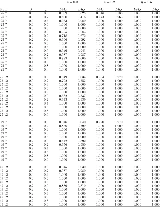
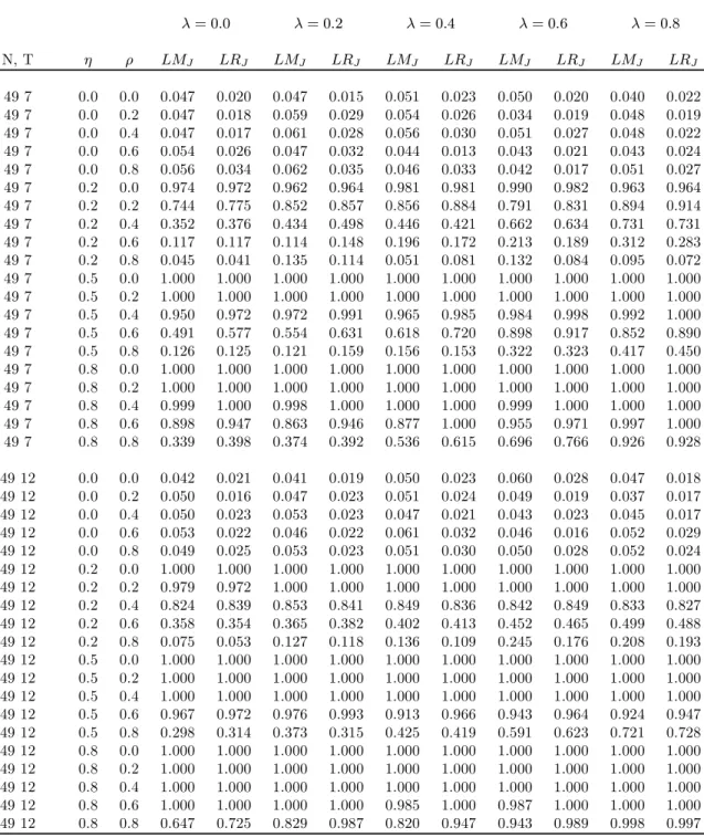
Table 1 gives the frequency of rejections at the 5% level for the joint LR and LM tests for H0a: λ=ρ=σ2µ= 0.For1000replications, counts between37and63are not significantly different from 50 at the .05 level. The results are reported for N = 25, 49 and T = 7,
12 for the Rook weight matrix. Table 1 shows that at the 5% level, the size of the joint LR test is typically less than .05 and varies between 2.3% and 4% depending on N and T. In contrast, the size of the joint LM test is not significantly different from.05 varying between3.9% and4.9% depending onN and T. The power of the joint LM and LR tests is reasonably high as long asλor ρorη are larger than0.2. In fact, ifλor ρorη ≥0.4, this power is almost one in all cases. For afixedλ,ρorη, this power improves asN orT increase.
4.2
One-Dimensional Conditional Tests
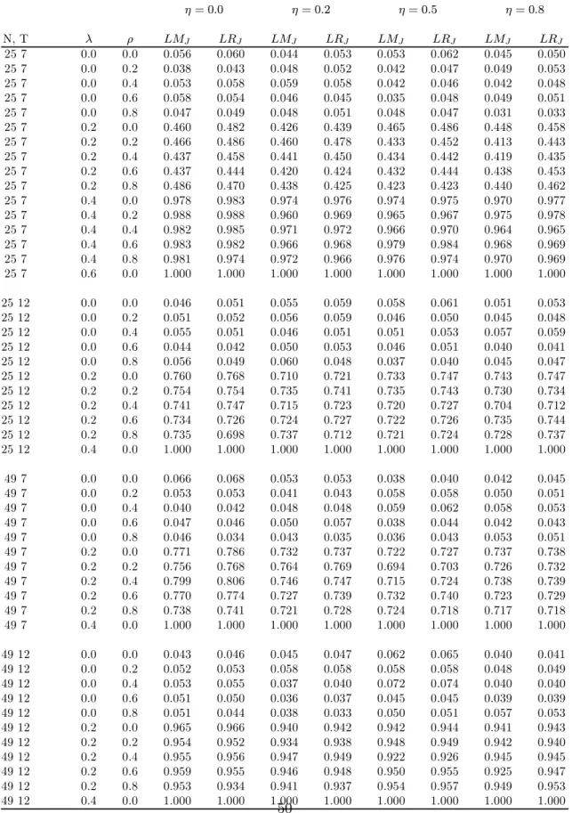
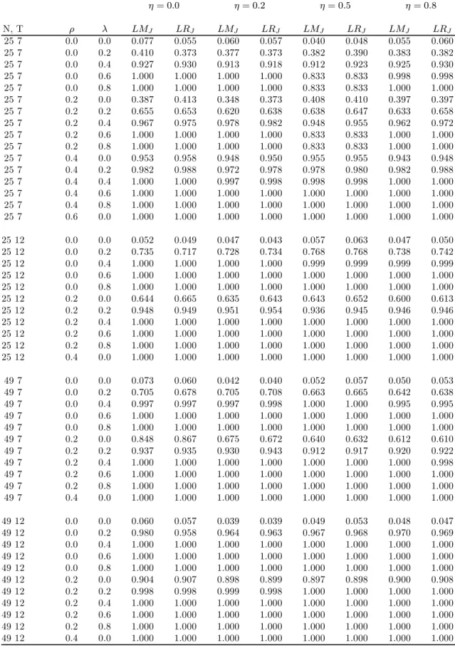
Table 2 gives the frequency of rejections at the 5% level for the one dimensional conditional LR and LM tests forH0h: λ= 0(assumingρ6= 0andσ2µ>0). The size of these conditional tests is not significantly different from .05 except in two cases. ForN = 25, T = 7, this varies between 3.1% and 5.9% for the LM test and 3.3% to 6.2% for the LR test. The power of these conditional LM and LR tests is reasonably high as long asλis larger than
0.2. In fact, if λ ≥ 0.4, this power is almost one in all cases. For a small λ= 0.2, this power improves as N orT increase.
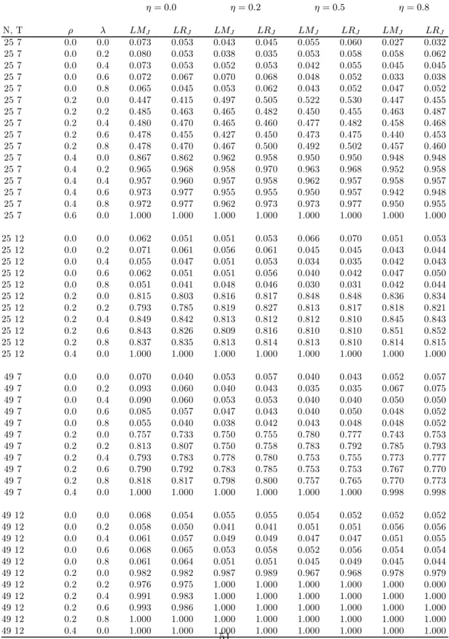
Table 3 gives the frequency of rejections at the 5% level for the one dimensional conditional LR and LM tests forHi
0: ρ= 0(assumingλ6= 0andσ2µ>0). The size of these conditional
tests is not significantly different from .05 except in a few cases, like when η = 0, where the LM test is oversized ranging from 6.5% to 8% for N = 25 and T = 7, and 5.5% to
9.3% forN = 49andT = 7.Things improve asT increases from7to12as expected. The LR test is better sized ranging from 4.0% to6.7% for η = 0 and all values of N and T. The power of these conditional LM and LR tests is close to one as long asρis larger than
0.2. For a smallρ= 0.2, this power improves asN orT increase.
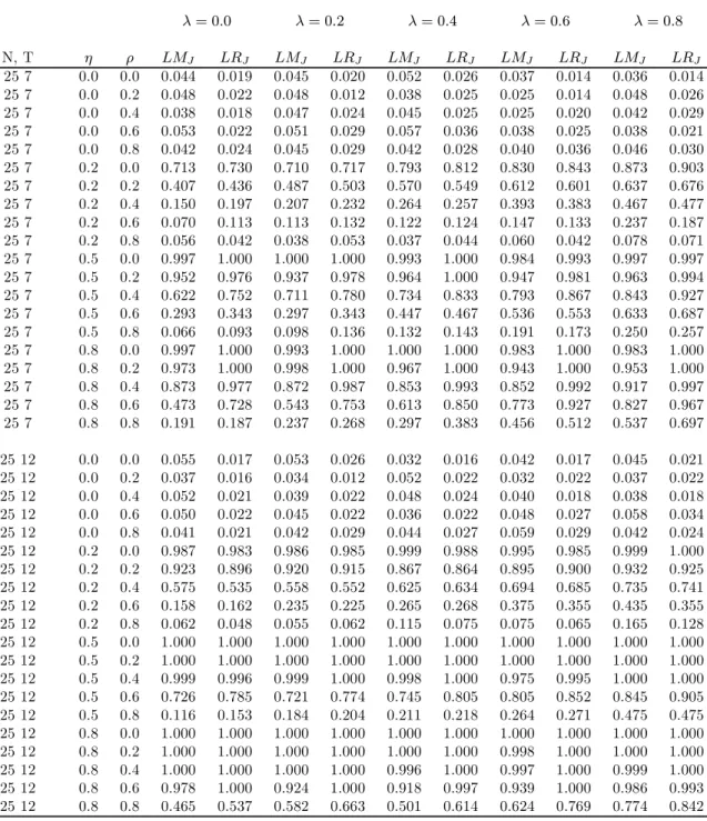
Table 4 gives the frequency of rejections at the 5% level for the one dimensional conditional LR and LM tests for H0j: σ2µ= 0(assuming ρ6= 0andλ6= 0). The LR test is undersized ranging from 1.6% to 3.4% for λ = 0 and all values of N and T. In contrast, the LM test is not significantly different from .05 for λ= 0 and all values ofN and T. The size of this LM test varies between 3.7% and 5.6%. The power of these conditional LM and LR tests increase with η, N and T. However, for a givenη and λ, there is a drop in the power as ρ becomes larger than 0.6, yielding low power for ρ= 0.8. Things improve as N orT increase. This may be due to the interaction effect between the serial correlation
over time due to the AR(1) process on the remainder disturbances and the constant serial correlation over time due to the same region effect.
4.3
Two-Dimensional Conditional Tests
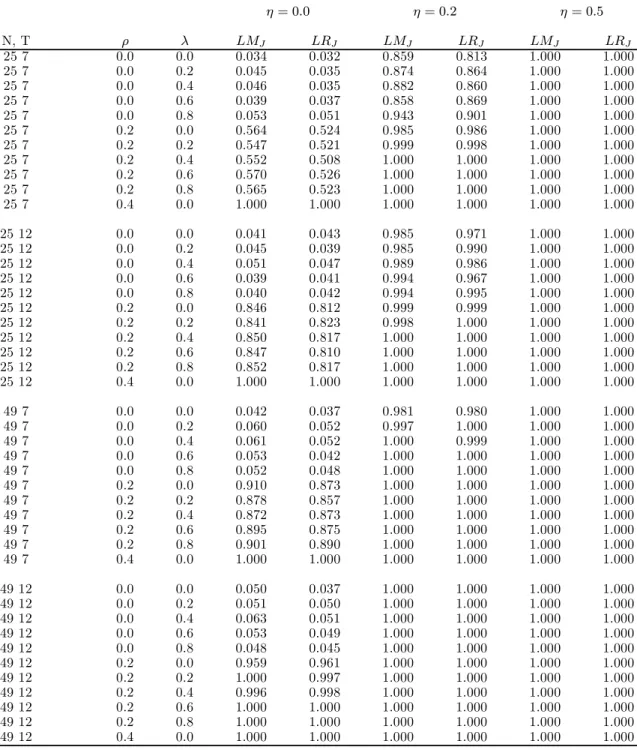
Table 5 gives the frequency of rejections at the 5% level for the two dimensional conditional LR and LM tests for Hk
0: λ = ρ = 0 (assuming σ2µ > 0). The size of these conditional
tests is not significantly different from.05 except for the LM test whenη= 0and T = 7. This varies between3.9% to 7.7% for the LM test and 3.9% to6.3% for the LR test. The power of these conditional LM and LR tests is close to one as long asλorρis larger than
0.2. For smallλ(orρ) = 0.2,this power improves asN,T orρ(λ) increase.
Table 6 gives the frequency of rejections at the 5% level for the two dimensional conditional LR and LM tests for H0l: λ=σ2µ = 0 (assumingρ6= 0). The LR test is undersized with size ranging from 2% to4.4%, while the LM test has size between 3.4% and5.9%. This is not significantly different from 5% except in two cases. The power of these conditional LM and LR tests is close to one as long as λ is larger than 0.2. For small λ= 0.2,this power improves as N or T or η increase. However, this increase in power with η is slow forρ= 0.8, and yields low power forT = 7. Things improve asT increases from7to12. Again this may be due to the interaction between the serial correlation due toρand that due toη.
Table 7 gives the frequency of rejections at the 5% level for the two dimensional conditional LR and LM tests for Hm
0 : σ2µ =ρ = 0(assuming λ6= 0). The LR test is undersized for
only 3 cases whenN = 25andT = 7and λ= 0,0.2,and 0.4.However, the size of the LR is not significantly different from 5% for larger N or T. The LM test is properly sized in all cases but one. This is for N = 25, T = 2and λ= 0. In all other cases, it is not significantly different from 5%. The power of these conditional LM and LR tests is close to one as long as λorρ is larger than0.2. For small ρ(orη) = 0.2,this power improves asN orT orη (orρ) increase.
5
Conclusion
This paper considered a spatial panel regresion model with serial correlation over time for each spatial unit and spatial dependence across these units at a particular point in time. In addition, the model allowed for heterogeneity across the spatial units through random effects. Testing for any one of these symptoms ignoring the other two is shown to lead to misleading results. The paper derived joint, conditional and marginal LM and LR tests for these symptoms and studied their performance using Monte Carlo experiments. This paper generalized the Baltagi and Li (1995) paper by allowing for spatial error correlation. It also generalized the Baltagi, Song and Koh (2003) paper by allowing for serial correlation over time. In effect, the tests derived in this paper encompass the earlier ones. Ignoring these correlations whether spatial at a point in time or serial correlation for a spatial unit over time may result in misleading inference. The paper does not consider alternative forms of spatial lag dependence and this should be the subject of future research. Also, the results in the paper should be tempered by the fact that theN = 25,49 used in our
Monte Carlo experiments may be small for a typical micro panel. LargerN will probably improve the performance of these tests whose critical values are based on their large sample distributions. However, it will also increase the computation difficulty and accuracy of the eigenvalues of the big weighting matrix W. Finally, it is important to point out that the asymptotic distribution of our test statistics were not explicitly derived in the paper but that they are likely to hold under a similar set of low level assumptions developed by Kelejian and Prucha (2001).
6
REFERENCES
Anselin, L. (1988). Spatial Econometrics: Methods and Models (Kluwer Academic Pub-lishers, Dordrecht).
Anselin, L. (1999). Rao’s score tests in spatial econometrics. Journal of Statistical Planning and Inference, (forthcoming).
Anselin, L. and A.K. Bera (1998). Spatial dependence in linear regression models with an introduction to spatial econometrics. In A. Ullah and D.E.A. Giles, (eds.),Handbook of Applied Economic Statistics, Marcel Dekker, New York.
Anselin, L and S. Rey (1991). Properties of tests for spatial dependence in linear regres-sion models. Geographical Analysis 23, 112-131.
Anselin, L. and R. Florax (1995). Small sample properties of tests for spatial dependence in regression models: Some further results. In L. Anselin and R. Florax, (eds.),New Directions in Spatial Econometrics, Springer-Verlag, Berlin, pp. 21-74.
Baltagi, B.H. (2001). Econometrics Analysis of Panel Data (Wiley, Chichester).
Baltagi, B.H. and Q. Li (1995). Testing AR(1) against MA(1) disturbances in an error component model. Journal of Econometrics 68, 133-151.
Baltagi, B.H., S.H. Song and W. Koh (2003). Testing panel data regression models with spatial error correlation. Journal of Econometrics 117, 123-150.
Bell, K.P. and N.R. Bockstael (2000). Applying the generalized-moments estimation approach to spatial problems involving microlevel data. Review of Economics and Statistics 82, 72-82.
Breusch, T.S. and L.G. Godfrey (1981). A review of recent work on testing for autocor-relation in dynamic simultaneous models. In D.A. Currie, R. Nobay and D. Peels, (eds.),Macroeconomic Analysis, Essays in Macroeconomics and Economics, Croom, Helm, London, pp. 63-100.
Breusch, T.S. and A.R. Pagan (1980). The Lagrange Multiplier test and its application to model specification in econometrics. Review of Economic Studies 47, 239-254. Case, A.C. (1991). Spatial patterns in household demand. Econometrica 59, 953-965. Conley, T.G. and G. Topa (2002). Socio-economic distance and spatial patterns in
Hartley, H.O. and J.N.K. Rao (1967). Maximum likelihood estimation for the mixed analysis of variance model. Biometrika 54, 93-108.
Harville, D.A. (1977). Maximum likelihood approaches to variance component estimation and to related problems.Journal of the American Statistical Association 72, 320-338. Hemmerle, W.J. and H.O. Hartley (1973). Computing maximum likelihood estimates for the mixed A.O.V. model using the W-transformation. Technometrics 15, 819-831. Holtz-Eakin, D. (1994). Public-sector capital and the productivity puzzle. Review of
Economics and Statistics 76, 12-21.
Kelejian, H.H. and I.R. Prucha (1999). A generalized moments estimator for the autore-gressive parameter in a spatial model. International Economic Review 40, 509-533. Kelejian, H.H. and I.R. Prucha (2001). On the asymptotic distribution of the Moran I
test with applications. Journal of Econometrics 104, 219-257.
Kelejian H.H and D.P. Robinson (1992). Spatial autocorrelation: A new computationally simple test with an application to per capita county police expenditures. Regional Science and Urban Economics 22, 317-331.
Magnus, J.R. (1982). Multivariate error components analysis of linear and nonlinear regression models by maximum likelihood. Journal of Econometrics 19, 239-285. Nerlove, M. (1971). Further evidence on the estimation of dynamic economic relations
from a time-series of cross-sections. Econometrica 39, 359-382.
Pinkse, J. (1998). Asymptotic properties of Moran and related tests and a test for spatial correlation in probit models. Working paper, Department of Economics, University of British Columbia.
Pinkse, J. (1999). Moran-flavoured tests with nuisance parameters: Examples. In L. Anselin and R.J.G.M. Florax (eds.),New Advances in Spatial Econometrics, (forth-coming).
Pinkse, J., M.E. Slade and C. Brett (2002). Spatial price competition: A semiparametric approach. Econometrica 70, 1111-1153.
Appendix A.1: Joint LM test for
ρ
=
λ
=
σ
2µ= 0
This appendix derives the joint LM test for spatial error correlation, random region effects andfirst-order serial correlation in the remainder error term. The null hypothesis is given by H0a: σ2µ = ρ = λ = 0. Let θ0 = (σ2e,σ2µ,ρ,λ). Note that the part of the information matrix corresponding toβ will be ignored in computing the LM statistic, since the infor-mation matrix is block diagonal between the θ and β parameters and thefirst derivative with respect toβ evaluated at the restricted MLE is zero. The LM statistic is given by:
LM = ˜D0θJ˜θ−1D˜θ (A.1)
whereD˜θ = (∂L/∂θ)(˜θ)is a4×1vector of partial derivatives of the likelihood function with
respect to each element ofθ, evaluated at the restricted MLE˜θ. Also,Jθ =E[−∂2L/∂θ∂θ0]
is the part of the information matrix corresponding to θ, and J˜θ is Jθ evaluated at the
restricted MLE˜θ. Under the null hypothesisH0a, the variance-covariance matrix given in (2.7) reduces to Ω0 = σ2eIT ⊗IN and the restricted MLE of β is β˜OLS, so that u˜ =y−
Xβ˜OLS are the OLS residuals andσ˜2e = ˜u0u/N T˜ . Hartley and Rao (1967) and Hemmerle and Hartley (1973) give a general useful formula that helps in obtaining D˜θ:
∂L ∂θr =-1 2tr · Ω−1∂Ω ∂θr ¸ +1 2u 0 µ Ω−1∂Ω ∂θr Ω−1 ¶ u (A.2)
forr = 1,2,3,4. It is easy to show from (2.7) that∂Ω/∂σ2e=Vρ⊗(B0B)−1,∂Ω/∂σ2µ=JT⊗
IN and ∂Ω/∂λ=V ⊗(B0B)−1(W0B+B0W)(B0B)−1 using the fact that∂(B0B)−1/∂λ= (B0B)−1(W0B+B0W)(B0B)−1,see Anselin (1988, p.164). ∂V
1/∂ρ|Ha
o =G, where G is a bidiagonal matrix with bidiagonal elements all equal to one.
Ω−1|Ha 0 = 1 σ2 e IT ⊗IN (A.3) (∂Ω/∂σ2e)|Ha 0 =IT ⊗IN (A.4) (∂Ω/∂σ2µ)|Ha 0 =JT ⊗IN (A.5) (∂Ω/∂ρ)|Ha 0 =σ 2 e(G⊗IN) (A.6) (∂Ω/∂λ)|Ha 0 =σ 2 eIT ⊗(W0+W) (A.7)
This uses the fact that, under H0a, B = IN and V1 = IT. Using (A.2), the score with
respect to each element of θ, evaluated at the restricted MLE is given by
˜ D1= D(˜σ2e) D(˜σ2µ) D(˜ρ) D(˜λ) = 0 N T 2˜σ2 e ¡u˜0(JT⊗IN)˜u ˜ u0u˜ −1 ¢ N T 2 ˜ u0(G⊗IN)˜u ˜ u0u˜ N T 2 ˜ u0(IT⊗(W0+W))˜u ˜ u0u˜ (A.8)
Using the following matrix differentiation formula given in Harville (1977): Jrs=E h − ∂ 2L ∂θr∂θs i = 1 2tr h Ω−1∂Ω ∂θr Ω−1∂Ω ∂θs i for r, s= 1,2,3,4. (A.9)
one gets the information matrix underH0a: ˜ Jθ = N T 2˜σ4e 1 1 0 0 1 T 2(T−1)˜σ2e T 0 0 2(T−1)˜σ2e T 2(T−1)˜σ4e T 0 0 0 0 2bσ˜4e N (A.10)
where b = tr(W2 +W0W). Note that J˜θ is a block diagonal matrix with respect to (σ2e,σ2µ,ρ) and λ. Substituting (A.8) and (A.10) in (A.1), the resulting LM statistic is given by LMJ = N T2 2(T−1)(T−2)[A 2 −4AF + 2T F2] +N 2T b H 2 (A.11) where A = u˜0(JT⊗IN)˜u ˜ u0˜u −1, F = 12 ¡u˜0(G⊗IN)˜u ˜ u0u˜ ¢ and H = 12 ³ ˜ u0(IT⊗(W0+W))˜u ˜ u0u˜ ´ . Under the null hypothesisH0a, this LM statistic is asymptotically distributed as χ23.
Appendix A.2: Joint LR test for
ρ
=
λ
=
σ
2µ= 0
This appendix derives the LR test for the joint significance of spatial error correlation, random region effects andfirst-order serial correlation. Using (2.7), the variance-covariance matrix can be rewritten as
Ω=σ2eh(JT ⊗IN)φ+Vρ⊗(B0B)−1
i
=σ2eΣ
where φ=σ2µ/σe2, Vρ = 1−1ρ2V1, and V1 is defined in (2.8). In this case,Σ−1 =Ω−1/σ2e
withΣ∗−1 =Ω∗−1/σ2
e similarly defined. Ω∗ is given by (2.12). In fact,
Σ∗−1= ¯JTα⊗Z0+ETα⊗(B0B) (A.12)
whereZ0 = [d2(1−ρ)2φIN+ (B0B)−1]−1=σ2eZ. UsingΩ∗= (C⊗IN)Ω(C0⊗IN), we get
Σ−1 = [C0⊗IN]Σ∗−1[C⊗IN] = Vρ−1⊗(B0B) + 1 d2(1−ρ)2 ¡ Vρ−1JTVρ−1 ¢ ⊗[Z0−(B0B)] (A.13) where d2 = α2+ (T −1) and α = q 1+ρ
1−ρ. This uses the fact that CιT = (1−ρ)ι α T and C0C=V−1 ρ .Also, |Σ∗|=|d2(1−ρ)2φIN + (B0B)−1| · |(B0B)−1|T−1, (A.14) and using Σ= [C⊗IN]Σ∗[C0⊗IN] (A.15) we get |Σ|=|Σ∗|/(1−ρ2)N (A.16)
Therefore, under the normality assumption of the disturbances, the log-likelihood function can be written as L = Const.−1 2ln|Ω ∗|+1 2u ∗0Ω∗−1 u∗ = Const.−N T 2 lnσ 2 e− 1 2ln|Σ ∗|− 1 2σ2 e u∗0Σ∗−1u∗ = Const.+N 2 ln(1−ρ 2) −12ln|d2(1−ρ)2φIN + (B0B)−1|− N T 2 lnσ 2 e +(T−1) ln|B|− 1 2σ2 e u0Σ−1u (A.17)
Thefirst-order conditions give closed form solutions for βˆ and σˆ2e conditional onλ,ˆ φˆ and
ˆ ρ: ˆ β = (X0Σ−1X)−1X0Σ−1y, (A.18) ˆ σ2e = (y−Xβ)0Σ−1(y−Xβ)/N T. (A.19)
Following Hemmerle and Hartley(1973), we get from (A.11) that ∂Σ ∂ρ = ∂ ∂ρ µ 1 1−ρ2V1 ¶ ⊗(B0B)−1 = µ 2ρ (1−ρ2)2V1+ 1 1−ρ2Fρ ¶ ⊗(B0B)−1 = 1 1−ρ2 (2ρVρ+Fρ)⊗(B0B)− 1 (A.20) where Fρ= ∂V1 ∂ρ = 0 1 2ρ · · · (T −1)ρT−2 1 0 1 · · · (T −2)ρT−3 .. . ... ... ... ... (T−1)ρT−2 (T−2)ρT−3 (T −3)ρT−4 · · · 0 (A.21)
Therefore, using (A.13) and (A.20), we get ∂L ∂ρ = − 1 2tr · Σ−1∂Σ ∂ρ ¸ + 1 2σ2 e u0 µ Σ−1∂Σ ∂ρΣ −1 ¶ u = −Nρ/(1−ρ2) −2d2(1 1 −ρ)2(1−ρ2)[4ρ(1−ρ) + 2ρ(T −2)(1−ρ) 2+ 2(1 −ρ2)(T −1)] {tr¡d2(1−ρ)2φ(B0B) +IN ¢−1 −N} + 1 2(1−ρ2)σ2 e ˆ u0¡Σ−1£(2ρVρ+Fρ)⊗(B0B)−1 ¤ Σ−1¢uˆ (A.22) where Σ−1∂Σ ∂ρ = 1 1−ρ2(2ρIT +V− 1 ρ Fρ)⊗IN + 1 d2(1−ρ)2(1−ρ2) ¡ 2ρVρ−1JT +Vρ−1JTVρ−1Fρ ¢ ⊗n¡d2(1−ρ)2φ(B0B) +IN ¢−1 −IN o (A.23) tr · Σ−1∂Σ ∂ρ ¸ = 2ρN (1−ρ2) + 1 d2(1−ρ)2(1−ρ2) [4ρ(1−ρ) + 2ρ(T−2)(1−ρ)2+ 2(1−ρ2)(T−1)] {tr¡d2(1−ρ)2φ(B0B) +IN ¢−1 −N} (A.24)
using the fact that tr[Vρ−1JT] = (1−ρ){2 + (T−2)(1−ρ)}, tr[Vρ−1Fρ] =−2ρ(T−1)and
tr[V−1 ρ JTVρ−1Fρ] = 2(1−ρ)2(T−1). Σ−1∂Σ ∂ρΣ −1 = Σ−1£(2ρV ρ+Fρ)⊗(B0B)−1 ¤ Σ−1/(1−ρ2) = 1 1−ρ2Σ −1£(2ρV ρ+Fρ)⊗(B0B)−1¤Σ−1
Similarly, ∂L ∂φ = − 1 2tr[Σ −1∂Σ ∂φ] + 1 2σ2 ν u0Σ−1∂Σ ∂φΣ −1u (A.25) = −T 2tr h (TφIN+ (B0B)−1)−1 i + 1 2σ2 ν u0hJT ⊗(TφIN + (B0B)−1)−2 i u using ∂Σ ∂φ =JT ⊗IN Σ−1∂Σ ∂φ = ³ Vρ−1⊗(B0B) + 1 d2(1−ρ)2 ¡ Vρ−1JTVρ−1 ¢ ⊗[Z0−(B0B)] ´³ JT ⊗IN ´ = Vρ−1JT ⊗(B0B) + 1 d2(1−ρ)2V −1 ρ JTVρ−1JT ⊗[Z0−(B0B)] tr[Σ−1∂Σ ∂φ] = (1−ρ){2 + (T−2)(1−ρ)}tr(B 0B) (A.26) + 1 d2(1−ρ)2[(1−ρ){2 + (T−2)(1−ρ)}] 2tr[Z 0−(B0B)] = · k2− k2 2 d2(1−ρ)2 ¸ tr(B0B) + k 2 2 d2(1−ρ)2 tr(Z0), wherek2 = (1−ρ){2 + (T−2)(1−ρ)}. Σ−1∂Σ ∂φΣ −1 = ³V−1 ρ JT ⊗(B0B) + 1 d2(1−ρ)2V −1 ρ JTVρ−1JT ⊗[Z0−(B0B)] ´ ³ Vρ−1⊗(B0B) + 1 d2(1−ρ)2V −1 ρ JTVρ−1⊗[Z0−(B0B)] ´ (A.27) Also, ∂L ∂λ = − 1 2tr h (TφIN + (B0B)−1)−1(B0B)−1(W0B+B0W)(B0B)−1 i −T −2 1trh(W0B+B0W)(B0B)−1i+ 1 2σ2 ν u0hΣ−1∂Σ ∂λΣ −1iu. (A.28) using ∂Σ ∂λ =Vρ⊗(B 0B)−1(W0B+B0W)(B0B)−1 (A.29) Σ−1∂Σ ∂λ =IT ⊗(W 0B+B0W)(B0B)−1 (A.30) + 1 d2(1−ρ)2V− 1 ρ JT ⊗[Z0−(B0B)](B0B)−1(W0B+B0W)(B0B)−1
tr¡Σ−1∂Σ ∂λ ¢ =T tr³(W0B+B0W)(B0B)−1´ + 1 d2(1−ρ)2(1−ρ){(1−ρ)(T−2) + 2} · © tr[Z0(B0B)−1(W0B+B0W)(B0B)−1]−tr[(W0B+B0W)(B0B)−1] ª (A.31) The Fisher scoring procedure is used to estimate φ, λ and ρ. Using the formula in Harville(1977), the elements of the information matrix corresponding to φ, λ and ρ can be obtained from the expressions derived above. For example
Eh− ∂ 2L ∂φ2 i = 1 2tr h Σ−1∂Σ ∂φ i2 = T 2 2 tr hn TφIN + (B0B)−1 o−2i (A.32) and Eh− ∂ 2L ∂ρ2 i = 1 2tr h Σ−1∂Σ ∂ρ i2 = T 2 2 tr hn TφIN + (B0B)−1 o−2i (A.33) Starting with an initial value, the (r+ 1)th updated value ofλ,φand ρare given by
ˆ λ ˆ φ ˆ ρ r+1 = ˆ λ ˆ φ ˆ ρ r + E[−∂∂λ2L2] E[−∂ 2L ∂λ∂φ] E[− ∂2L ∂λ∂ρ] E[−∂λ∂φ∂2L ] E[−∂∂φ2L2] E[−∂ 2L ∂φ∂ρ] E[−∂λ∂ρ∂2L] E[−∂φ∂ρ∂2L] E[−∂∂ρ2L2] −1 r ∂L ∂λ ∂L ∂φ ∂L ∂ρ (A.34)
where at each step,∂L/∂λ,∂L/∂φand∂L/∂ρare obtained from equations (A.28), (A.25) and (A.22). βˆ and σˆ2e are obtained from (A.18) and (A.19), and the information matrix is obtained from equations like (A.32-A.33). The subscriptr means that these terms are evaluated at the estimates of therth iteration.
Appendix A.3: (M.4) LM test for
H
0e:
λ
=
ρ
= 0
given
σ
2µ= 0
When σ2
µ = 0, the variance-covariance matrix in (2.7) reduces to Ω = σ2eVρ⊗(B0B)−1.
UnderH0e: λ=ρ= 0givenσ2µ= 0,Ω reduces toΩ0 =σ2eIT ⊗IN withΩ−01 = σ12
eIT ⊗IN. ∂Ω ∂σ2 e| He 0 =IT ⊗IN ∂Ω ∂ρ|H0e =σ 2 eG⊗IN ∂Ω ∂λ|H0e =σ 2 eIT ⊗(W +W0) Also, Ω−1 ∂Ω ∂σ2 e |He 0 = 1 σ2 eIT ⊗IN tr · Ω−1 ∂Ω ∂σ2 e ¸ |He 0 = N T σ2 e Ω−1 ∂Ω ∂σ2 e Ω−1| He 0 = 1 σ4 eIT ⊗IN Using (A.2), we get
∂L ∂σ2 e |He 0 =− N T 2σ2 e + 1 2σ4 e ˆ u0[IT ⊗IN] ˆu= 0 Similarly, Ω−1∂Ω ∂ρ|H0e =G⊗IN tr · Ω−1∂Ω ∂ρ ¸ |He 0 = 0 Ω−1∂Ω ∂ρΩ −1 |He 0 = 1 σ2 e G⊗IN
Using (A.2), we get ∂L ∂ρ|H0e = 1 2σ2 e ˆ u0[G⊗IN] ˆu Finally, Ω−1∂Ω ∂λ|H0e =IT ⊗(W 0+W) tr · Ω−1∂Ω ∂λ ¸ |He 0 = 0 Ω−1∂Ω ∂λΩ −1| He 0 = 1 σ2 e IT ⊗(W0+W)
Using (A.2), we get ∂L ∂λ|H0e = 1 2σ2 e ˆ u0£IT ⊗(W0+W) ¤ ˆ u
Using (A.9), the elements of the information matrix under H0e are given by: J11 = E · − ∂ 2L ∂(σ2 e)2 ¸ = 1 2tr · 1 σ4 e IT ⊗IN ¸ = N T 2σ4 e J12 = E · − ∂ 2L ∂σ2 e∂ρ ¸ = 1 2tr · 1 σ2 e G⊗IN ¸ = 0 J13 = E · − ∂ 2L ∂σ2 e∂λ ¸ = 1 2tr · 1 σ2 e IT ⊗(W+W0) ¸ = 0 J22 = E · −∂ 2L ∂ρ2 ¸ = 1 2tr h G2⊗IN i =N(T −1) J23 = E · − ∂ 2L ∂ρ∂λ ¸ = 1 2tr £ G⊗(W+W0)¤= 0 J33 = E · −∂ 2L ∂λ2 ¸ = 1 2tr £ IT ⊗(W0+W)2 ¤ =T tr(W2+W0W)
So the score vector is given by (A.8) with D(˜σ2
µ) deleted. Similarly, the information
matrix is given by (A.10) with the 2nd row and column deleted. The resulting matrix is diagonal which leads to the result thatLMλρ =LMλ+LMρ.
Appendix A.4: (M.5) LM test for
H
0f:
λ
=
σ
2µ
= 0
given
ρ
= 0
When ρ= 0, the variance-covariance matrix in (2.7) reduces toΩ=σ2µJT ⊗IN +σ2eIT ⊗ (B0B)−1. Under H0f: λ = σ2µ = 0 given ρ = 0, Ω reduces to Ω0 = σ2eIT ⊗IN with
Ω−01= σ12 eIT ⊗IN. ∂Ω ∂σ2 e|H f 0 =IT ⊗IN ∂Ω ∂σ2 µ |Hf 0 =JT ⊗IN ∂Ω ∂λ|H0f =σ 2 eIT ⊗(W +W0) Also, Ω−1 ∂Ω ∂σ2 e |Hf 0 = σ12 eIT ⊗IN tr · Ω−1 ∂Ω ∂σ2 e ¸ |Hf 0 = N T σ2 e Ω−1 ∂Ω ∂σ2 e Ω−1|Hf 0 = 1 σ4 e IT ⊗IN
Using (A.2), we get ∂L ∂σ2 e|H f 0 =− N T 2σ2 e + 1 2σ4 e ˆ u0[IT ⊗IN] ˆu= 0 Similarly, Ω−1 ∂Ω ∂σ2 µ|H f 0 = 1 σ2 e JT ⊗IN tr · Ω−1 ∂Ω ∂σ2 µ ¸ |Hf 0 = N T σ2 e Ω−1 ∂Ω ∂σ2 µ Ω−1|Hf 0 = 1 σ4 e JT ⊗IN
Using (A.2), we get ∂L ∂σ2 µ |Hf 0 =−N T 2σ2 e + 1 2σ4 e ˆ u0[JT ⊗IN] ˆu= N T 2ˆσ2e µ ˆ u0(JT ⊗IN)ˆu ˆ u0ˆu −1 ¶ Finally, Ω−1∂Ω ∂λ|H0f =IT ⊗(W0+W) tr · Ω−1∂Ω ∂λ ¸ |Hf 0 = 0 Ω−1∂Ω ∂λΩ− 1| H0f = 1 σ2 e IT ⊗(W0+W)
Using (A.2), we get ∂L ∂λ|H0f = 1 2σ2 e ˆ u0£IT ⊗(W0+W) ¤ ˆ u
Using (A.9), the elements of the information matrix under H0f are given by: J11 = E · − ∂ 2L ∂(σ2 e)2 ¸ = 1 2 tr · 1 σ4 e IT ⊗IN ¸ = N T 2σ4 e J12 = E · − ∂ 2L ∂σ2 e∂σ2µ ¸ = 1 2tr · 1 σ4 e JT ⊗IN ¸ = N T 2σ4 e J13 = E · − ∂ 2L ∂σ2 e∂λ ¸ = 1 2 tr · 1 σ2 e IT ⊗(W +W0) ¸ = 0 J22 = E · − ∂ 2L ∂(σ2 µ)2 ¸ = 1 2 tr h 1 σ4 e JT2 ⊗IN i = N T 2 2σ4 e J23 = E · − ∂ 2L ∂σ2 µ∂λ ¸ = 1 2 tr · 1 σ2 e JT ⊗(W+W0) ¸ = 0 J33 = E · −∂ 2L ∂λ2 ¸ = 1 2 tr £ IT ⊗(W0+W)2 ¤ =T tr(W2+W0W).
So, the score vector is given by (A.8) withD(˜ρ)deleted. Similarly, the information matrix is given by (A.10) with the 3rd row and column deleted. Simple inversion of this block diagonal information matrix leads toLMλµ=LMλ+LMµ.
Appendix A.5: (M.6) LM test for
H
0g:
σ
2µ=
ρ
= 0
given
λ
= 0
Whenλ= 0, the variance-covariance matrix in (2.7) reduces toΩ=σ2
µJT⊗IN+σ2eVρ⊗IN.
UnderH0g: σ2µ=ρ= 0given λ= 0,Ωreduces toΩ0=σ2eIT ⊗IN withΩ−01 = σ12
eIT ⊗IN. ∂Ω ∂σ2 e |H0g =IT ⊗IN ∂Ω ∂σ2 µ|H g 0 =JT ⊗IN ∂Ω ∂ρ|H0g =σ 2 eG⊗IN Also, Ω−1 ∂Ω ∂σ2 e|H g 0 = 1 σ2 e IT ⊗IN tr · Ω−1 ∂Ω ∂σ2 e ¸ |H0g = N T σ2 e Ω−1 ∂Ω ∂σ2 e Ω−1|Hg 0 = 1 σ4 e IT ⊗IN ∂L ∂σ2 e|H g 0 =− N T 2σ2 e + 1 2σ4 e ˆ u0[IT ⊗IN] ˆu= 0 Similarly, Ω−1 ∂Ω ∂σ2 µ|H g 0 = 1 σ2 e JT ⊗IN tr · Ω−1 ∂Ω ∂σ2 µ ¸ |H0g = N T σ2 e Ω−1 ∂Ω ∂σ2 µ Ω−1|Hg 0 = 1 σ4 e JT ⊗IN
Using (A.2), we get ∂L ∂σ2 µ|H g 0 =− N T 2σ2 e + 1 2σ4 e u0[JT ⊗IN]u= N T 2ˆσ2e µ ˆ u(JT ⊗IN)ˆu ˆ u0uˆ −1 ¶ Ω−1∂Ω ∂ρ|H0g =G⊗IN tr · Ω−1∂Ω ∂ρ ¸ |H0g = 0 Ω−1∂Ω ∂ρΩ −1 |H0g = 1 σ2 e G⊗IN
Using (A.2), we get ∂L ∂ρ|H0g = 1 2σ2 e u0[G⊗IN]u
Using (A.9), elements of the information matrix under H0g are given by: J11 = E · − ∂ 2L ∂(σ2 e)2 ¸ = 1 2tr · 1 σ4 e IT ⊗IN ¸ = N T 2σ4 e J12 = E · − ∂ 2L ∂σ2 e∂σ2µ ¸ = 1 2tr · 1 σ4 e JT ⊗IN ¸ = N T 2σ4 e J13 = E · − ∂ 2L ∂σ2 e∂ρ ¸ = 1 2tr · 1 σ2 e G⊗IN ¸ = 0 J22 = E · − ∂ 2L ∂(σ2 µ)2 ¸ = 1 2tr h 1 σ4 e JT2⊗IN i = N T 2 2σ4 e J23 = E · − ∂ 2L ∂σ2 µ∂ρ ¸ = 1 2tr · 1 σ2 e JTG⊗IN ¸ = N(T −1) σ2 e J33 = E · −∂ 2L ∂ρ2 ¸ = 1 2tr h G2⊗IN i = N 2 2(T −1) =N(T−1)
So, the score is given by (A.8) withD(˜λ)deleted. Also, the information matrix is given by (A.10) with the 4th row and column removed. Inverting the resulting information matrix and computing the LM statistic, we get LMµρ.
Appendix A.6: (C.1) LM test for
H
0h:
λ
= 0
given
ρ
6
= 0
and
σ
2µ>
0
Under H0h: λ = 0 given ρ 6= 0 and σ2µ > 0, Ω in (2.7) reduces to Ω0 = σ2µ(JT ⊗IN) +
σ2e(Vρ⊗IN)with Ω−01= (V−1−cV−1JTV−1)⊗IN wherec= σ 2 eσ2µ d2(1−ρ)2σ2 µ+σ2e d2=α2+ (T −1), α= r 1 +ρ 1−ρ ∂Ω ∂σ2 e |Hh 0 =Vρ⊗IN = 1 σ2 e V ⊗IN Ω−1∂Ω ∂σ2 e |Hh 0 = 1 σ2 e (IT −c V−1JT)⊗IN tr · Ω−1∂Ω ∂σ2 e ¸ |Hh 0 =N(T−cg)/σ 2 e whereg=tr(V−1JT) = (1σ−2ρ) e {2 + (T−2)(1−ρ)}. Ω−1∂Ω ∂σ2 e Ω−1|Hh 0 = ³ 1 σ2 e (IT −c V−1JT)⊗IN ´³ V−1−c V−1JTV−1⊗IN ´ = 1 σ2 e ³ V−1−2c V−1JTV−1+ [c V−1JT]2V−1 ´ ⊗IN
Using (A.2), we get ∂L ∂σ2 e |Hh 0 = − N 2σ2 e [T −cg] + 1 2σ2 e ˆ u0h³V−1−2c V−1JTV−1+ [c V−1JT]2V−1 ´ ⊗IN i ˆ u Similarly, ∂Ω ∂σ2 µ|H h 0 =JT ⊗IN Ω−1 ∂Ω ∂σ2 µ|H h 0 = ³ V−1JT −c(V−1JT)2 ´ ⊗IN tr · Ω−1 ∂Ω ∂σ2 µ ¸ |Hh 0 =Ng(1−cg) Ω−1 ∂Ω ∂σ2 µ Ω−1|Hh 0 = (V −1 −c V−1JTV−1)JT(V−1−c V−1JTV−1)⊗IN
Using (A.2), we get ∂L ∂σ2 µ |Hh 0 = − N 2 Ã (1−ρ) σ2 e {2 + (T−2)(1−ρ)}−c · (1−ρ) σ2 e {2 + (T −2)(1−ρ)} ¸2! +1 2u 0£(V−1 −c V−1JTV−1)JT(V−1−c V−1JTV−1)⊗IN ¤ u ∂Ω ∂ρ|H0h=σ 2 e · 2ρ (1−ρ2)2V1+ 1 1−ρ2Fρ ¸ ⊗IN =σ2eHρ⊗IN whereHρ= h 2ρ (1−ρ2)2V1+1−1ρ2Fρ i =h2ρVρ+Fρ 1−ρ2 i
andFρis defined in (A.21).
Ω−1∂Ω ∂ρ|H0h=σ 2 e ¡ V−1−c V−1JTV−1 ¢ Hρ⊗IN tr · Ω−1∂Ω ∂ρ ¸ |Hh 0 =Nσ 2 etr £¡ V−1−c V−1JTV−1 ¢ Hρ ¤ Ω−1∂Ω ∂ρΩ −1 |Hh 0 =σ 2 e h¡ V−1−c V−1JTV−1 ¢ Hρ ¡ V−1−c V−1JTV−1 ¢i ⊗IN
Using (A.2), we get ∂L ∂ρ|H0h = − Nσ2e 2 tr £¡ V−1−c V−1JTV−1 ¢ Hρ ¤ + σ 2 e 2 u 0h¡V−1 −c V−1JTV−1 ¢ Hρ ¡ V−1−c V−1JTV−1 ¢ ⊗IN i u ∂Ω ∂λ|H0h=V ⊗(W 0+W) Ω−1∂Ω ∂λ|H0h = ³ V−1−c V−1JTV−1⊗IN ´³ V ⊗(W0+W) ´ = (IT −c V−1JT)⊗(W0+W) tr · Ω−1∂Ω ∂λ ¸ |Hh 0 = 0 Ω−1∂Ω ∂λΩ −1 |Hh 0 = ¡ V−1−c V−1JTV−1 ¢ V¡V−1−c V−1JTV−1 ¢ ⊗(W0+W)
Using (A.2), we get ∂L ∂λ|H0h = ˆD(λ) = 1 2u 0£V−1 −2c V−1JTV−1+c2[V−1JT]2V−1 ¤ ⊗(W0+W)u
which is given in (3.5). Using (A.9), elements of the information matrix under H0h are given by:
J11 = 1 2tr · 1 σ2 e (IT −c V−1JT)⊗IN ¸2 = N 2σ4 e tr£IT −2c V−1JT +c2V−1JTV−1JT ¤ = N 2σ4 e £ T−2cg+ (cg)2¤ J12 = 1 2tr ·³ 1 σ2 e (IT −c V−1JT)⊗IN ´³ (V−1JT −c V−1JTV−1JT)⊗IN ´¸ = N 2σ2 e tr£V−1JT −2c(V−1JT)2+c2(V−1JT)3 ¤ = N 2σ2 e (g−2cg2+c2g3) = N 2σ2 e g(1−cg)2 J13 = 1 2tr ·³ 1 σ2 e (IT −c V−1JT)⊗IN ´³ σ2e¡V−1−c V−1JTV−1 ¢ Hρ⊗IN ´¸ = 1 2tr £ V−1Hρ−2c V−1JTV−1Hρ+c2(V−1JT)2V−1Hρ ¤ J14 = 1 2tr h³1 σ2 e (IT −c V−1JT)⊗IN ´³ (IT −c V−1JT)⊗(W0+W) ´i = 0 J22 = 1 2tr[(V −1J T −c V−1JTV−1JT)⊗IN]2 = N 2 tr[(V −1J T)2−2c (V−1JT)3+c2 (V−1JT)4] = N 2g 2(1 −cg)2 J23 = 1 2tr h³ (V−1JT −c V−1JTV−1JT)⊗IN ´³ σ2e¡V−1−c V−1JTV−1 ¢ Hρ⊗IN ´i = Nσ 2 e 2 tr h¡ V−1JTV−1−2c(V−1JT)2V−1+c2(V−1JT)3V−1 ¢ Hρ i J24 = 1 2tr h³ (V−1JT −c(V−1JT)2)⊗IN ´³ (IT −c V−1JT)⊗(W0+W) i = 0
J33 = 1 2tr £ σ2e¡V−1−c V−1JTV−1 ¢ Hρ⊗IN ¤2 = Nσ 4 e 2 tr £¡ V−1−c V−1JTV−1 ¢ Hρ ¤2 J34 = 1 2tr h³ σ2e¡V−1−c V−1JTV−1 ¢ Hρ⊗IN ´³ (IT −c V−1JT)⊗(W0+W) ´i = 0 J44 = 1 2tr h (IT −c V−1JT)⊗(W0+W) i2 = 1 2tr[(IT −2cV −1J T +c2( V−1JT)2)⊗(W0+W)(W0+W)] = b(T−2cg+c2g2) where tr[V−1Hρ] = 2ρ σ2 e(1−ρ2) .
Appendix A.7: LM test for
H
0i:
ρ
= 0
given
λ
6
= 0
and
σ
2µ>
0
UnderHi
0: ρ= 0given λ6= 0and σ2µ>0,Ωin (2.7) reduces to
Ω0=σ2µJT ⊗IN +σ2eIT ⊗(B0B)−1
replacingJT byTJ¯T andIT by ET + ¯JT, we get
Ω0= ¯JT ⊗ £ Tσ2µIN +σ2e(B0B)−1 ¤ +σ2eET ⊗(B0B)−1 Hence Ω−01= 1 σ2 e ET ⊗(B0B) + ¯JT ⊗Z whereZ = [Tσ2µIN +σe2(B0B)−1]−1. ∂Ω ∂σ2 e|H i 0 =IT ⊗(B 0B)−1 Ω−1∂Ω ∂σ2 e |Hi 0 = 1 σ2 e (ET ⊗IN) + ¯JT ⊗Z(B0B)−1 tr · Ω−1∂Ω ∂σ2 e ¸ |Hi 0 = (T −1)N σ2 e +tr[Z(B0B)−1] Ω−1∂Ω ∂σ2 e Ω−1|Hi 0 = 1 σ4 e ET ⊗(B0B) + ¯JT ⊗Z(B0B)−1Z
Using (A.2), we get ∂L ∂σ2 e |Hi 0 = − 1 2 · (T−1)N σ2 e +tr[Z(B0B)−1] ¸ +1 2u 0 · 1 σ4 e ET ⊗(B0B) + ¯JT ⊗Z(B0B)−1Z ¸ u ∂Ω ∂σ2 µ|H i 0 =T ¯ JT ⊗IN Ω−1 ∂Ω ∂σ2 µ |Hi 0 = µ 1 σ2 e ET ⊗(B0B) + ¯JT ⊗Z ¶¡ TJ¯T ⊗IN ¢ =TJ¯T ⊗Z tr · Ω−1 ∂Ω ∂σ2 µ ¸ |Hi 0 =Ttr[Z] Ω−1 ∂Ω ∂σ2 µ Ω−1|Hi 0 = ¡ TJ¯T ⊗Z ¢µ 1 σ2 e ET ⊗(B0B) + ¯JT ⊗Z ¶ =TJ¯T ⊗Z2
Using (A.2), we get ∂L ∂σ2 µ|H i 0 =− T 2tr[Z] + T 2u 0( ¯J T ⊗ZZ)u