This is an Open Access document downloaded from ORCA, Cardiff University's institutional repository: http://orca.cf.ac.uk/115408/
This is the author’s version of a work that was submitted to / accepted for publication. Citation for final published version:
Mohammed, Ahmed, Harris, Irina, Soroka, Anthony and Nujoom, Reda 2019. A hybrid MCDM-fuzzy multi-objective programming approach for a G-Resilient supply chain network design.
Computers and Industrial Engineering 127 , pp. 297-312. 10.1016/j.cie.2018.09.052 file Publishers page: http://dx.doi.org/10.1016/j.cie.2018.09.052
<http://dx.doi.org/10.1016/j.cie.2018.09.052> Please note:
Changes made as a result of publishing processes such as copy-editing, formatting and page numbers may not be reflected in this version. For the definitive version of this publication, please refer to the published source. You are advised to consult the publisher’s version if you wish to cite
this paper.
This version is being made available in accordance with publisher policies. See
http://orca.cf.ac.uk/policies.html for usage policies. Copyright and moral rights for publications made available in ORCA are retained by the copyright holders.
1
A hybrid MCDM-fuzzy multi-objective programming approach for a G-Resilient supply chain network design
Abstract
Stakeholders are being increasingly encouraged to improve their supply chain risk management in order to cope efficiently and successfully with risk of disruption due to unexpected events. However, green development was overlooked when considering environmental impact which has become a main criterion in supply chain management. Where the era of greenness threatens current supply chain partners with the need to either cope with the new green regulations or leave the field for new players. Thus, an approach to design supply chains that are simultaneously resilient, and green is needed. This study satisfies this need by developing a green and resilient (G-resilient, here after) fuzzy multi-objective programming model (GR-FMOPM) to present a G-resilient supply chain network design in determining the optimal number of facilities that should be established. The objectives are minimization of total cost and environmental impact and maximization of Value of resilience pillars where Redundancy, Agility, Leanness and Flexibility (V-RALF) are four of the main pillars of supply chain resilience. Fuzzy AHP is used for determining the importance weight for each pillar followed by the application of a Fuzzy technique for assigning the importance weight for each potential facility with respect to RALF. The importance weights obtained by Fuzzy AHP and the Fuzzy technique are then integrated in the third objective (maximization of V-RALF) to maximize the value of resilience pillars. Based on the fuzzy multi-objective model, the ε-constraint method is used to reveal Pareto optimal solutions and TOPSIS was then used to select the final Pareto solution. A case study is used to validate the applicability of the developed GR-FMOPM in obtaining a G-resilient supply chain network design and a trade-off among economic, green and resilience objectives. Finally, a sensitivity analysis is performed on the importance weight for facilities Pareto solutions with respect to the importance weight of RALF. Research findings proved that the developed GR-FMOPM could be used as a tool in evaluating and ranking related facilities with respect to their resilience performance. It can also be used to obtain a G-resilient supply chain network design in terms of facilities that should be established towards a trade-off among the three aforementioned objectives.
Keywords: G-Resilient; Green development; Supply chain resilience; Fuzzy multi-objective
2
1. Introduction
Recently, the focus of supply chain resilience has gained a growing interest by supply chain managers and academics due to significant incidents happening around the world (Soni et al., 2014; Reyes Levalle and Nof, 2015). The major concerns are how to improve their supply chain risk management to generate a resilient supply chain that can efficiently pre-empt and react to disruptions due to unexpected incidents (e.g. natural disasters and variance in demands and supply). Unexpected disruptions in the flow of information, merchandise, and services can happen due to incidents such earthquakes, floods, etc., and can lead to a failure in supply chain’s performance in terms of satisfying customers’ demands at the right time and right location. For instance, the earthquake that happened in Japan in 2007 lead to significant damage to the area where Toyota's key suppliers were located. Therefore, Toyota had to shut down production in 12 plants due to lack of supplies (Pettit et al., 2010). Supply chain managers of IBM reported that risk management ranks as the second main concern for them (IBM, 2008). A study accomplished by Computer Sciences Organisation reported that 60% of the surveyed enterprises stated that their supply chains are subject to disruptions. Moreover, 46% of the supply chain managers acknowledged that effective supply chain risk management is required (Hillman and Keltz, 2007). Thereafter, a limited number of enterprises have taken steps to generate resilient supply chains (Muthukrishnan and Shulman, 2006).
The increasing concern of environmental problems for supply chain management has led to an expansion of the boundaries of awareness from conventional to green supply chain networks. Carbon dioxide (CO2) levels are one of the main environmental factors that negatively affect
the climate where growing energy consumption leads to an increase of the effect (Jabbar, 2008). Thus, decreasing CO2 emissions has become of paramount importance for industries,
particularly in the USA, the European Union countries, and Japan, due to altered consumer behaviour that seeks green services and goods.
Supply chain managers and researchers are being tasked to improve supply chain resilience to cope with disruption risks. They have lagged behind this target, overlooking green development in considering environmental impact which has become a main criteria in supply chain management and vice versa. Where the era of greenness forces current supply chain partners to either adapt to the new green regulations or to leave the field for new players. A survival plan is to develop an integrated approach which is simultaneously resilient enough to efficiently cope with unexpected disruptions and green in order to handle the increasing global
3
requirement to decrease environmental impacts. Rose (2011) argued that disruptions could significantly influence the environment, which interrupts the main processes of a supply chain network. One of the main hurdles in obtaining a green supply chain is the vagueness related to supply chain processes. Consequently, resilience should be integrated with green supply chains to handle uncertainty from disruptions (Rosa et al., 2013). Perrings (2006) clarifies that sustainability and resilience are two of the main key-effects in growing economies. Therefore, the potential approach should also consider the total costs required for the design the supply chain networks aiming to present a cost-effective, green and resilient design.
In the context of resilience pillars, Ponomarov and Holcomb (2009) reviewed the literature and proposed some elements to create a resilient supply chain. Rajesh and Ravi (2015) investigated the relationships among the enablers of supply chain risk mitigation in an electronic supply chain using the grey DEMATEL approach. The authors recently presented a supplier selection study considering resilience pillars such as flexibility, supply capability and supplier profile. Kamalahmadi and Mellat-Parast (2016) argued that the flexibility of supplier capability could be an effective strategy to improve resilience. Rice and Caniato (2003) differentiated redundancy from flexibility. Redundancy capacity is an additional capacity that can be used to replace the loss of capacity caused by a disturbance. Flexibility, on the other hand, entails restructuring previously existing capacity. Purvis et al. (2016) proposed a framework for the development and implementation of a resilient supply chain strategy, which illustrates the relevance of various management paradigms (robustness, agility, leanness and flexibility).
Several research papers have accomplished generating a resilient supply chain network (Carvalho et al., 2012; Pereira et al., 2014; Nooraie and Parast, 2015; Mari et al., 2014; Rezapour et al., 2017) and a green supply chain network (Paksoy et al., 2012; Kannan et al., 2013; Harris et al., 2014; Talaei et al., 2015; Tiwari et al., 2016; Mohammed and Wang, 2017 and 2017a; Miranda-Ackerman et al., 2017). On the other hand, the reviewed literature shows that none or few of the previous studies have presented an integrated approach which is both simultaneously resilient in terms of robustness, agility, leanness and flexibility to efficiently cope with unexpected disruptions, and green to handle the increasing global requirements in decreasing the environmental impact.
This study presents the development of a multi-objective programming model to design a G-resilient supply chain network in solving the allocation problem of related facilities. Regarding resilience, this work considers four pillars (enablers) as key factors to improve supply chain
4
resilience including redundancy, agility, leanness and flexibility as proposed by Purvis et al. (2016). The importance weight for each pillar is determined using Fuzzy AHP and the correspondence weight for each potential facility is then determined using a fuzzy technique based on decision makers’ expertise. Afterwards, the determined importance weights are integrated in the developed multi-objective model to maximize the value of resilience considering the four pillars. The developed model aims to simultaneously optimize three objectives: minimization of total operation, administration, transportation and purchasing cost, minimization of environmental impact in CO2 emissions related to transportation throughout
the network and opening related facilities and maximization of V-RALF. To cope with the vagueness in some of the input parameters (e.g. purchasing costs, purchasing quantities, demands, CO2 emissions and capacity of facilities), the multi-objective model is then
developed in the term of a fuzzy multi-objective model. The ε-constraint method is employed to optimize the three objectives simultaneously in terms of revealing a set of Pareto optimal solutions. Finally, TOPSIS is employed to help decision makers in selecting the final Pareto solution.
To the best of the authors’ knowledge, this research is the first attempt in developing an approach that presents a resilient (considering the main pillars of supply chain resilience) and green supply chain network design using multi criteria decision-making and multi-objective optimization approaches. Furthermore, none of the previous studies have used multi criteria decision-making techniques (e.g. AHP or Fuzzy AHP) to assign the related weights for resilience enablers (e.g. robustness, agility, leanness and flexibility) and integrate them in a fuzzy multi-objective optimization model aiming to maximize value of resilient.
The structure of the paper is as follows. Selected literature is reviewed in Section 2. The problem and research methodology are illustrated in Section 3. The developed fuzzy multi-objective model and its optimization methodology is described in in Section 4. The results and discussions are presented in Section 5. Finally, conclusions and avenues for future directions are drawn in Section 6.
2. Literature review
The reviewed literature revealed that some research MCDMs for designing and optimizing supply chains network design has already been conducted (Harris et al., 2014; Talaei et al., 2015; Mohammed and Wang, 2017a). This section has reviewed related studies that used MCDM in green supply chains and supply chain resilience.
5 2.1 MCDM in green supply chains
Several research studies have employed multi-objective optimization for handling the environmental impacts of supply chain network design. Kelly et al. (2013) reviewed five approaches that can be used for assessing and managing environmental responsibilities. Elbounjimi et al. (2014) analysed a literature review of the mathematical models used to design green closed-loop supply chain networks. Eskandarpour et al. (2015) presented a literature survey study on facility location problem reviewing 87 academic papers which taking into account economic and ecological aspects and discussing several optimization methodologies. Furthermore, the authors categorized the papers based on the modelling type e.g. single objective, multi-objective, deterministic, stochastic, and non-linear. Recently, Govindan et al. (2017) reviewed research in the field of green supply chain network design under uncertainty. Elhedhli and Ryan (2012) formulated a model for solving a supply chain design problem with respect to CO2 emissions due to transportation throughout the chain. Bing et al. (2015)
proposed a mathematical optimization model programing for optimizing re-allocation of intermediate processing plants considering emission constraints. Entezaminia et al. (2016) developed a multi-objective programming model for obtaining a green supply chain network design considering the environmental impacts. Li et al. (2017) solved a two-echelon supply chain network design problem considering the production and transportation outsourcing problems restricted to the cap-and-trade policy and carbon tax policy. Garg et al. (2015) proposed a bi-objective integer nonlinear programming for solving closed-looped four echelons supply chain networks taking into account the environmental issues. Sahar et al. (2014) modelled a multi-objective programming model that aims at minimizing CO2 emissions
of transportation and the total cost for a dairy supply chain network. Paksoy et al. (2012) proposed a fuzzy multi-objective model for a green closed-loop supply chain network in minimizing transportation costs and CO2 emissions. Soleimani et al. (2017) solved a facility
location problem of a supply chain considering environmental aspect via the development of a objective optimization model. Miranda-Ackerman et al. (2017) developed a multi-objective-TOPSIS model with an aim of obtaining a green three echelons Orange Juice supply chain. Golpîra et al. (2017) formulated a green opportunistic supply chain network design problem under uncertain input parameters (e.g., demands and shortage costs) as a robust multi-objective mixed integer linear programming. Shaw et al. (2016) formulated a supply chain network design model considering carbon emissions and carbon trading issues. Benders approach was proposed to solve the optimization problem. Pishvaee et al. (2014) developed a
6
multi-objective possibilistic programming to solve a sustainable facility location problem under uncertainty. Mallidis et al. (2014) formulated a multi-objective optimization model to investigate the impact of optimizing facility location and inventory planning on the cost and CO2 emissions of multi-layer logistics networks. Coskun et al. (2015) solved an environmental sustainability supply chain network design problem encountring the customer segmentation. Goal programming was applied to cope with various conflicting targets e.g., total cost, green responsibilities and shortages cost.
2.2 MCDM in supply chain resilience
The study of supply chain resilience has drawn substantial interest from researchers. In this context, there are several papers in the literature that used multi-objective optimization is minimizing disruption risk which aims to generate a more resilient supply chain. Snyder et al. (2011) proposed a stochastic multi-objective model for solving a facility location problem considering facility disruptions. Azaron et al. (2008) investigated a three-echelon supply chain in obtaining a compromised solution among total cost, total cost variance, and financial risk cost by the goal attainment technique. Hatefi and Jolai (2014) developed a robust model for a closed-loop network design under facility disruption risk and uncertain demand. Nooraie et al. (2015) formulated a multi-objective model that includes minimization of investment costs, minimization of the variance of the total cost and minimization of the financial risk aiming to obtain a trade-off among them. Dixit et al. (2016) proposed a multi-objective model to maximize supply chain resilience in minimizing unfulfilled demand and transportation cost post-disaster. The RALF framework, Purvis et al. (2016), demonstrated the application of a qualitative supply chain resilience assessment technique within the food and drink sector based on a “traffic light” system. Where a matrix of 16 key company activities (such as: ingredient sourcing, production planning and logistics control) versus the four key management paradigms that create resilience (robustness, agility, leanness and flexibility) is used to evaluate companies. Each activity is qualitatively assessed (against the perceived industry norm) and then assigned a score that is interpreted into a “traffic light”, from 1 (worst = red) to 5 (best = green).
The literature review revealed that research has been conducted into generating resilient supply chain networks and green supply chain networks (Paksoy et al., 2012; Kannan et al., 2013; Harris et al., 2014; Talaei et al., 2015; Tiwari et al., 2016; Mohammed and Wang, 2016). Table
7
1 lists a number of important studies that use various approaches to obtain green and resilient supply chains.
However, the reviewed literature showed that sustainability and resilience aspects have been considered individually (Redman, 2014) as none of the previous studies have presented an integrated approach which is simultaneously resilient in terms of robustness, agility, leanness and flexibility to efficiently cope with unexpected disruptions and green to handle the increasing global requirements in decreasing the environmental impact. The only three studies found in the literature considering resilience and green aspects was presented by Mari et al. (2014); Fahimnia and Jabbarzadeh (2016) and Zahiri et al. (2017). Mari et al. (2014) proposed a multi-objective model that simultaneously optimizes total cost, disruption costs and carbon emissions throughout a supply chain network. Zahiri et al. (2017) developed a possibilistic-stochastic multi-objective optimization model to design a pharmaceutical supply chain network considering sustainability and unexpected disruptions. Similarly, Fahimnia and Jabbarzadeh (2016) formulated a stochastic fuzzy goal programming to embed sustainability and resilience responsibilities into supply chain network. The resilience aspect was formulated based on probability of disruption occurrence. However, the two studies did not consider (1) the main resilience pillars in designing the supply chain network that we consider in this study, (2) the weight of each resilience pillars, (3) the integration of importance weight of resilience pillars into the multi-objective model, and (4) the model formulated by Mari et al. (2014) did not handle the uncertainty in the input parameters. Thus, this study enriches related literature in green supply chain and supply chain resilience in several ways. It presents the development of a green and resilient fuzzy multi-objective model to obtain a green and resilient supply chain network design with respect to multiple uncertainties. Also, it incorporates the main pillars of supply chain resilience in the developed fuzzy multi-objective model. Moreover, it allocates an importance weight for each resilience pillar (i.e. RALF) and for each potential facility correspondence to these pillars using multi criteria design-making techniques.
8 Table 1. A review of the literature
References
Dimensions
Techniques
Resilience Green
This study * * Fuzzy AHP + TOPSIS +
Multi-objective optimization
Mari et al. (2014) * * Multi-objective
optimization
Fahimnia and Jabbarzadeh (2016)
* * Stochastic fuzzy goal
programming
Zahiri et al. (2017) * * Possibilistic-stochastic
multi-objective optimization
Carvalho et al. (2012) * Simulation
Nooraie and Parast (2015) * Multi-objective
optimization
Kannan et al. (2015) * FAD
Mohammed et al. (2018) Gencer and Gürpinar (2007)
* ANP
Kuo et al. (2010) * ANN + MADA + DEA
Awasthi and Kannan (2016)
* Fuzzy NGT + VIKOR
Shaw et al. (2012) * Fuzzy AHP+Fuzzy,
Multi-objective optimization
9
Tsui and Wen (2014) * AHP+ELECTRE
Harris et al. (2015) * Multi-objective
optimization
Fallahpour et al. (2016) * DEA + Genetic
programming
Luthra et al. (2017) * AHP and VIKOR
Soni et al. (2014) * Mathematical modelling
Pettit et al. (2013) * Supply Chain Resilience
Assessment and
Management (SCRAM™)
Aryanezhad et al. (2010) * Expected Value
approach
Chen et al. (2011) * Expected Value
approach
Sawik (2014, 2015) * Stochastic mixed integer
programming
Hosseini and Barker (2016)
* Bayesian Network (BN)
Lee (2009) * Fuzzy AHP
Madadi et al. (2014) * Conditional
value-at-risk (CVaR)
Hernandez et al. (2014) * Multi-objective
optimization
Peng et al. (2011) * Multi-objective
10
Baroud et al. (2015) * Stochastic programming
Losada et al. (2012) * Mathematical modelling
Rezapour et al. (2017) * Mixed integer non-linear
modelling
3. Problem description and research methodology
Fig. 1 illustrates the supply chain under study which consists of three sets of facilities E, F and G. This research aims at supporting decision makers in obtaining a G-resilient supply chain network design in allocating the optimal number of facilities E and F that should be established with respect to green and resilience performance. Thus, multi criteria decision-making techniques and the developed multi-objective optimization model are integrated. Firstly, fuzzy AHP is used to assign importance weights for the four pillars (i.e. robustness, agility, leanness and flexibility) of supply chain resilience. Secondly, a fuzzy technique is used to allocate an importance weight for facilities E and F with respect to the four resilience pillars. Thirdly, the obtained weights from fuzzy AHP and the fuzzy technique are incorporated in a developed multi-objective model that aims at minimizing total cost and environmental impact and maximizing V-RALF. To cope with the fuzziness in some of the input parameters (e.g. purchasing costs, purchasing quantities, demands, CO2 emissions and capacities of facilities),
the multi-objective model is then developed in terms of a fuzzy multi-objective model. Fourthly, the ε-constraint method is used to obtain a set of Pareto optimal solutions. Finally, TOPSIS was employed to select the final Pareto solution. Figure 2 shows a framework in terms of the processes followed for developing a hybrid MCDM-fuzzy multi-objective programming approach towards a G-resilient supply chain network design.
11
Fig.1 Structure of the supply chain network under study.
mfg 1 2 g G Set of Facilities G tfg 1 2 f F Set of Facilities F 1 2 e E Set of facilities E mef tef
12
Apply TOPSIS to select the final solution Apply fuzzy AHP to weight resilience pillars
Solve the model using the ε-constraint Start
Identify a set of eligible facilities E & F
G-resilient supply chain network design Formulate the multi-objective model:
Min total cost
Min environmental impact
Max the value of supply chain resilience Apply Eqs. 1-3 to weight facilities in terms of resilience
pillars
Assign ε-values Identify and define resilience pillars
Model the uncertainty by formulating the fuzzy multi-objective model
Solve the three objective functions individually to obtain their maximum and minimum values
13
Fig. 2. A framework of the developed GR-FMOPM used for obtaining a G-resilient supply
chain network design.
3.1 Obtaining the importance weights
In this research, fuzzy AHP is used to determine the importance weight for each resilience pillar. Fuzzy AHP is a decision-making algorithm presented by incorporating Saaty’s AHP approach developed in the 1970s with fuzzy set theory (Saaty, 2000; Zimmermann, 2010). In this algorithm, fuzzy numbers are presented by a membership function that is a real number between 0 and 1. Several research works have proved its applicability in solving related problem in supply chains and logistics (Shaw et al., 2012; Kannan et al., 2013; Li et al., 2013; Viswanadham and Samvedi, 2013; and Junior et al., 2014). Table 2 presents the linguistic variables used for evaluating the four pillars. Decision makers need to evaluate the importance of each pillar using the given linguistic variables. The Fuzzy AHP is applied as presented in Appendix A.
Table 2. Linguistic variables used for weighting resilience pillars
Linguistic Variable Fuzzy number
Equally important (EI) (0, 0.1, 0.3)
Weakly important (WI) (0.1, 0.3, 0.5)
Strongly more important (SMI) (0.3, 0.5, 0.7)
Very strongly important (VSI) (0.5, 0.7, 0.9)
Extremely important (EI) (0.7, 0.9, 0.10)
Afterwards, the weight of each potential facility with respect to each resilience pillar is determined as follows:
1. Build the decision matrix (MD) based on decision makers’ expertise as shown in Eq. 1.
Table 3 presents the linguistic variables used for evaluating facilities E and F with respect to each resilience pillar based on decision makers’ expertise.
1 2 ( n n ... Ln) D w w w M N (1)
Where N is the number of decision makers who evaluate the resilience performance of a particular facility (l).
14
2. Build the normalized decision matrix as follows:
l l D ND D l L RowM M RowM
(2)3. Determine the weight of each potential facility in terms of each resilience pillar by building the weighted normalized decision matrix as follows:
l l WN l L w RowM
(3)Where MWNl is the weighted normalized decision matrix obtained by multiplying the
normalized decision matrix (MMD) by the weight of resilience pillars obtained by using fuzzy
AHP.
Table 3. Linguistic variables used for weighting facilities E and F with respect to RALF
Linguistic Variable Fuzzy number
Very Low (VL) (0, 1, 3) Low (L) (1, 3, 5) Medium (M) (3, 5, 7) High (H) (5, 7, 9) Very High (VH) (7, 9, 10) 4. GR-FMOPM formulation
This section presents the development of a fuzzy multi-objective programming model used for obtaining a G-resilient network design for a supply chain. This model helps decision makers in determining the optimal number of facilities E and F that should be established with respect to economic, green and resilient responsibilities. The objectives include minimization of the total cost (O1), environmental impacts (O2), and maximization of value of robustness, agility, leanness and flexibility (V-RALF) (O3).
The GR-FMOPM model for the supply chain problem is formulated based on the following basic assumptions:
15
Critical parameters such as purchasing and transportation costs, CO2
emission/vehicle/m, purchasing quantities of abattoirs, demands of retailers and capacity levels of facilities are assumed to be uncertain.
Facilities F and G have different purchasing function in term of purchasing quantities and demands.
The supply chain under study is a forward supply chain network.
The potential locations of facilities are known.
The number of facilities G is fixed and known.
There is no product transportation between facilities at the same level i.e., between two facilities E.
Sets, parameters and decision variables were used for formulating the GR-FMOPM presented in Appendix B.
The first objective O1 minimizes the total cost, which comprises cost for purchasing product 1 from facilities E and product 2 facilities F, operating cost for running facilities E and F, administration cost at facilities E and F, transportation cost for product 1 from facility E to F and for the product 2 from facility F to G, respectively. In this model, transportation cost is formulated as transportation cost per unit (ceft andctfg) multiplied by transportation distance among facilities (tef and tfg) and number of required transportation vehicles, which is determined by quantity flow of products among facilities (mef andmfg) divided by truck transportation capacity (cl). With regards to the operating cost, it is determined by multiplying the labourer/hour cost by the number of working hours and then multiplied by a variable of number of labourer/hour required to process the transported quantity of products. Also, this
model was applied to an existing case study where the facilities are already existing. Therefore,
the facility establishment cost was not considered. Minimization of O1 is formulated as
follows: 1 ep ef pf fg ea ef af fg ef fg o o t t e e e E f e f f f ef F f F g G e E f F f F g G e E f F e E f F g e G f F f fg fg l l Min O c m c m c m c m m m c n x c n x c t c t c c
(4)16
The second objective O2 minimizes the environmental impact, which comprises the minimization of CO2 emissions due to running network facilities E and F and transporting
product 1 and 2 from facility E to F and from facility F to G, respectively. The minimization of O2 is formulated as follows: 2 _ 2 _ 2 _ 2 _ 2 e e f f ef ef ef fg fg fg e E f F e E f F l f F g G l m m Min O CO y CO y CO t CO t c c
(5)The third objective O3 maximizes the value of supply chain resilience in term of maximizing resilience pillars i.e. robustness (R), agility (A), leanness (L) and flexibility (F). The importance weights for each pillar and each facility (with respect to the four pillars) obtained by using the fuzzy AHP and the fuzzy technique are used to formalize the maximization of V-RALF. The maximization of O3 is formulated as follows:
3 eR eR e Rf Rf f eA eA e e E f F e E A A L L L L f f f e e e f f f f F e E f F F e E f F e E f F e E f F f f f e F F F e E f F e e e E e E wd wd wd wd wd w M d wd wd ax O w y w y w y w y w y w y w y w y
(6) Subject to: (7) (8) e e E f f m p
(9) (10) g G f mfg p
(11) (12) eÎ Eå
mef £ ceye f F fÎ Få
mfg £ cfyf " gÎ G f F fÎ Få
mfg ³ dg g G f F fÎ Få
mef £ xere e E17 f fg f f g G m x r F
(13) (14) (15)Where, Eq. 7 restricts the quantity of product 1 transported from facility E to F so that it cannot exceed the capacity of facility E. Eq. 8 ensures the quantity flow of product 2 from facility F to G does not exceed the capacity of facility F. Eqs. 9-11 ensure that the purchasing quantities of facility F and demands of facility G are fulfilled from facility E and F, respectively. Eqs. 12 and 13 indicate the required number of labourers (xe and xf) at facilities E and F. These were formulated as decision variables and determined based on working rate per labourer/day (re and rf) (i.e., how many unit labourer/day can handle) that can handle quantity flows of products
(me and mf). In other words, these terms refer to the total labourer/hour required to process a
specified quantity of products. This helps in limiting operating cost to the required number of labourer-hour to handle quantity flows of products rather determine it based on a fixed number of labourers that could probably be less or over the required number of labourers to run the facility. In the field of operation management, this is also so-called man/hour. Eqs. 14 and15 limit the non-binary and non-negativity restrictions on decision variables.
4.1 Formulating the fuzzy multi-objective model
To come closer to the real design, a number of input parameters including purchasing and transportation costs, purchasing quantities, demands, CO2 emissions throughout the
transportation activities and capacity levels of related facilities were considered as uncertain input parameters. Therefore, the multi-objective programming model previously developed in the previous section is re-developed as a fuzzy multi-objective programming model employing an approach developed by Jiménez et al. (2007). The equivalent crisp model is formulated as follows (Jiménez et al., 2007; and Mohammed and Wang, 2017a, Mohammed et al., 2017):
, 0 , , ef fg m m e f g , {1, 0}, , e f y y e f
18 4 4 2 1 2 4 2 e E f F f F g G e E f F f F g G
p pes p mos p opt p pes p mos p opt
f f f
e e e
ef fg
a a
e ef f fg
t pes t mos t opt
ef ef ef ef o o e e e f e E f F e E f f ef l F f c c c c c Min O m m c m c m c c c m c n x c n x t c C
4 2t pes t mos t opt
g fg fg fg fg fg l G f F c c c m t c
(16) 2 _ 2 _ 2 _ 2 _ 2 _ 2 2 _ 2 _ 2 _ 4 4 2 2 2 e e f f e E f Fpes mos opt
ef ef ef ef
ef ef
e E f F l
pes mos opt
fg fg fg fg fg f F g G l Min O CO y CO y CO CO CO m CO t c CO CO CO m t c
(17) 3 eR eR e Rf Rf f e E f F A A A A e e e f f f e E f F L L L L e e e f f f e E f F F e E f F e E f F F F F e e e e E f F f f f e E e E f F e E wd wd wd wd wd w Max O w y w y w y w y w y w y w d wd y wd w y
(18) Subject to:19 (19) (20) 1 2 3 4 . 1 , 2 2 2 2 e f f f E f ef m p p p p
(21) 1 2 3 4 . 1 , 2 2 2 2 f f f f g fg G p p p p m
(22) (23) (24) (25) (26) (27)According to Jiménez et al. (2007), the constraints in the multi-objective model that include uncertain parameters in supply capacity (see Eq. 7 and 8), purchasing quantities and demands (see Eqs. 9-11) should be fulfilled with a confidence value which is presented as α which is normally assigned by decision makers. The α value is associated with the uncertain parameters which include capacity of related facilities (Eqs. 19 and 20), purchasing quantities of facility F and demands of facility G (Eqs. 21-23). Also, mos, pes and opt are the three prominent points (the most likely, the most pessimistic and the most optimistic values), respectively.
4.1.1 GR-FMOPM Optimization
In order to optimize the developed GR-FMOPM, the flowing procedures are applied.
eÎ E
å
mef £ a 2. ce1+ce2 2 + 1-a 2 æ è ç ö ø ÷ce3+ce4 2 é ë ê ê ù û ú ú ye, f F fÎ Få
mef £ a 2. cf1+cf2 2 + 1 -a 2 æ è ç ö ø ÷cf3+cf4 2 é ë ê ê ù û ú ú yf, " gÎ G f F g G a 2. df1+df2 2 + 1 -a 2 æ è ç ö ø ÷df3+df4 2 é ë ê ê ù û ú ú ³ gÎ Gå
mfg, f F fÎ Få
mef £ xere e E gÎ Gå
mfg £ xfrf " f Î F , 0 , , ef fg m m e f g , , {1, 0}, , e f y y e f20
1. The linear membership function correspondence to each objective function is obtained as follows: 1 0 b b b b b b b b b b b b if A Max Min A if Min A Max Min Max if A Min (28)
where Ab represents the value of bth objective function and Maxb and Minb represent the
maximum and minimum values of bth objective function, respectably.
1.1. The minimum values for each objective are determined via optimizing each objective
individually as follows: 1 ep ef pf fg ea ef af fg ef fg o o t t e e e E f e f f f ef F f F g G e E f F f F g G e E f F e E f F g e G f F f fg fg l l Min O c m c m c m c m m m c n x c n x c t c t c c
(29) 2 _ 2 _ 2 _ 2 _ 2 e e f f ef ef ef fg fg fg e E f F e E f F l f F g G l m m Min O CO y CO y CO t CO t c c
(30) 3 eR eR e Rf Rf f e E f F A A A A e e e f f f e E f F L L L L e e e f f f e E f F F e E f F e E f F F F F e e e e E f F f f f e E e E f F e E wd wd wd wd wd w Min O w y w y w y w y w y w y w d wd y wd w y
(31)1.2. The maximum values for each objective are determined via optimizing each objective individually as follows:
21 1 ep ef fp fg ea ef af fg ef fg o o t t e e e E f e f f f ef F f F g G e E f F f F g G e E f F e E f F g e G f F f fg fg l l Max O c m c m c m c m m m c n x c n x c t c t c c
(32) 2 _ 2 _ 2 _ 2 _ 2 e e f f ef ef ef fg fg fg e E f F e E f F l f F g G l m m Max O CO y CO y CO t CO t c c
(33) 3 eR eR e Rf Rf f e E f F A A A A e e e f f f e E f F L L L L e e e f f f e E f F F e E f F e E f F F F F e e e e E f F f f f e E e E f F e E wd wd wd wd wd w Max O w y w y w y w y w y w y w d wd y wd w y
(34)2. The ε-constraint method is used to optimize the three objectives simultaneously. This method transforms the multi-objective model to a mono-objective model by keeping one of the functions as an objective function, and treating other functions as constraints limited to ε values (Ehrgott, 2005). The equivalent solution formula (O) is given by:
1 O Min O Min (35) Subject to: 2 1 O (36)
2 1
2 min max O O (37) 3 2 O (38)
3 2
3 min max O O (39) In addition to Eqs. 23-31.In this work, the total cost minimization is kept as an objective function (Eq. 35). Minimization of environmental impact and maximization of V-RALF is moved to ε-based constraints as presented in Eqs. 36 and 38, respectively. Different Pareto solutions can be generated by
22
varying values of ε1 and ε2. These values are varied between the maximum and minimum values of objectives three and two, respectively.
4.2 Revealing the final solution: TOPSIS
After obtaining a set of Pareto solutions, decision makers should select one solution to establish the number of facilities E and F. The selection of the final solution can be determined based on the decision makers’ preferences or using a decision-making algorithm. In this work, TOPSIS is used for helping the decision makers in selecting the final solution which is the closest to the ideal solution and furthest to the nadir solution. The application steps followed in Ramesh et al. (2012) are applied and discussed in Appendix C.
5. Evaluation of the GR-FMOPM: A case study
In this section, a case study of a meat supply chain, which encompasses 3 farms, 4 abattoirs and 7 retailers, is examined to evaluate the applicability of the developed fuzzy multi-objective programming model in solving a facility allocation problem with respect to economic, green and resilience responsibilities. In this chain, livestock is supplied from farms (set of facilities E) to abattoirs (set of facilities F) to be slaughtered then transported to retailers (set G) as a packed meat. Table 4 shows the input parameters used for the case study. For example, the supply capacity of farm e ( ) is given in a range 1,500 – 1,800 livestock. The data is collected from the meat committee in the UK (HMC). The travel distances between farms and abattoirs and between abattoirs and retailers are estimated using Google maps. Also, the demands and supply capacity of abattoirs and retailers reported in Table 4, is the total demand and capacity (livestock or meat packets) for a one-year period. It is worth mentioning that the CO2 emission per facility was collected from facilities environmental impact record. The later as illustrated by practitioners, it was estimated based on estimated CO2 per livestock (unit) which is based on national record in the UK. A decision maker (ADM) from an abattoir was asked to evaluate the importance of resilience pillars for the potential three farms (f1, f2 and f3) with respect to each pillar, and two decision makers (RDM1and RDM2) from two retailers were asked to evaluate the importance of resilience pillars and the potential four abattoirs (a1, a2, a3 and a4) with respect to each pillar. The decision makers have an average 9 years of work experience. A deep discussion (about 2 hours) was held with ADM, RDM1 and RDM2 individually to explain, discuss and evaluate resilience pillars and facilities. For the purposes of the study the following definitions were used in discussions with the decision makers:
23
Supply chain resilience “the ability of a [supply chain] to return to its original state or move
to a new, more desirable state after being disturbed” Christopher and Peck (2004). This would involve the meat supply chain network, shown in Fig. 1 earlier, being able to withstand and adapt to the shocks and stresses it is presented with.
Robustness measures the ability to withstand disruptions to elements within the supply
network, either through the immediate availability of alternative suppliers or being capable of quickly planning the incorporation of new suppliers. For example a retailer may have alternative suppliers available should an issue arise with a particular abattoir.
Agility evaluates the ability to respond in a quick and well-coordinated manner to
comparatively small market opportunities, through having a partner able to handle unexpected / volatile demand. An example would be an abattoir having several small specialist farms it can source from to help cope with demand peaks.
Leanness assesses the absence of excess / waste and hence the ability to fulfil predictable,
base-line, demand in an efficient manner. This could be a retailer that sources from several abattoirs that are able to efficiently and cost effectively meet a known base-level of demand.
Flexibility gauges the ability to respond easily to disturbances in the supply network, whilst
maintaining control of costs and lead-times. This involves having processes in place that enable effective response when disturbances in the supply chain are sensed, such as weather conditions that may prevent livestock from being taken to an abattoir for processing.
Finally, LINGO11 software is used for optimizing the GR-FMOPM running of a personal computer with a Corei5 3.2GHz processor and with 8GB RAM.
24 Table 4. Input parameters used for the case study
= 3 = 1-1.5 (GBP/Mile) = 110 – 205 (Mile) = 4 = 1-1.5 (GBP/Mile) = 50 (Unit/Vehicle) = 7 = 3 - 4.5 (GBP/unit) = 1500 – 1800 (Unit) = 130 – 150 (GBP/unit) = 3 - 4.5 (GBP/unit) = 1600 - 2000 (Unit) = 160 – 190 (GBP/unit) = 43 – 250 (Mile) ne = 9 (Hour) = 8 - 9.5 = 10 -11(GBP/Hour) nf = 9 (Hour) pf = 1250 – 1450 (Unit) CO2_ef = 271 – 294 (gram/Mile) CO2_e = 82000 – 85000 (Kg/facility) dg = 1100 – 1300 (Mile) CO2_fg = 271- 294 (gram/Mile) CO2_f = 220000 – 250000 (Kg/facility) = 60 (Unit/labourer-day) = 15 (Unit/labourer-day) 5.1 Results
The developed GR-FMOPM is optimized using the aforementioned input parameters as follows:
1. Table 5 shows the evaluation of the four resilience pillars based on decision makers’ expertise. As shown in Table 5, agility was evaluated as the most important pillar according the three decision makers’ expertise. On the other hand, leanness was evaluated the least important pillars. It is important to check the consistency in
decision makers’ opinions regarding the pairwise comparison among criteria. In this
context, Saaty developed a consistent indicator so-called Consistency Ratio (CR) that is used to determine whether decision makers’ evaluation is consistent. The consistency ratio is determined as CR = CI / RI; where CI refers to Consistency Index, and RI refers to Random Consistency Index. The pairwise comparison is considered to be consistent (or has an acceptable inconsistency) if the value of CR is less or equal to 0.1. The Consistency Index is determined as
E
c
ef tt
fgF
c
fg t c l G c e a ce cep cfac
fc
fpt
efc
eoc
of rer
f25 1 n CI n
; where n refers to the number of criteria; is determined by (i) finding the 3rd root for summation of each row in the pairwise decision matrix, (ii) determining the summation of the previous step, (iii) determining the summation of each column in the pairwise decision matrix, (iv) multiplying the summation by the criteria weight corresponding for each criterion, and (v) determine thevalue by
summing the values determined in the previous step. Finally, RI value corresponds to the number of criteria, further details, we refer the readers to (Saaty, 1994). In this work, CR1 = 0.0475/0.91 = 0.052 and CR2 = 0.031/0.91 = 0.034 which turned out an acceptable level of inconsistency for the first and second evaluations, respectively.
2. Fuzzy AHP is applied for allocating the importance weights of each resilience pillar including robustness, agility, leanness and flexibility based on decision makers’ expertise obtained in the previous step. Table 6 shows the obtained importance weight for each pillar. As shown in Table 6, the importance weight order is Agility>Robustness>Flexibility>Leanness based on ADM’s expertise, and Agility> Flexibility> Robustness>Leanness based on RDMs’ expertise.
3. Table 7 shows the evaluation of farms and abattoirs with respect to the four resilience pillars based on decision makers’ expertise. Eqs. 1-3 are then followed to determine the importance weights of the potential three farms and four abattoirs using the input parameters obtained from the previous step. Table 8 shows the results corresponding to the relevant pillars. Based on the obtained results, arguably, farm 2 (GW = 0.383483) and abattoir 3 (GW = 0.298397) revealed the highest resilience performance compared to farm 3 (GW = 0.272640) and abattoir 2 (GW = 0.214060) which revealed the worst resilience performance.
4. The three objective functions previously developed in section 4.1. are optimized simultaneously using the ε-constraint method as follows:
4.1. The minimum and maximum values for each objective are obtained via Eqs. 29-34, respectively. Table 9 shows the obtained objective values; for example, O1 {minimum, maximum} = {344,703, 501,868}. These values are used for assigning ε values and the correspondence membership functions for each objective.
4.2. Objective one (minimization of total cost) is left as an objective function and objectives two and three (minimization of environmental impact and maximization V-RALF, respectively) are shifted to the constraint.
26
4.3. The range between the maximum and minimum values for objective functions two and three are divided into ten points, the points in between are assigned as ε values in Eq. (36 and 38).
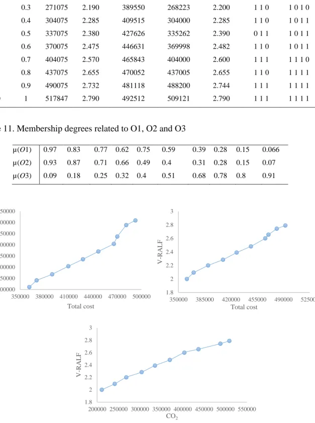
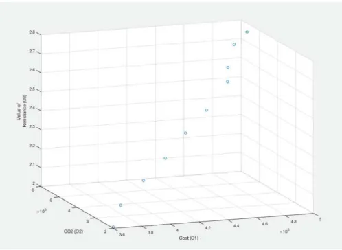
4.4. Pareto optimal solutions are obtained by applying Eq. 35. Table 10 shows a set of obtained Pareto optimal solutions which represent trade-offs amongst three objectives which include minimizing the total cost and environmental impact and maximization of V-RALF. Also, these solutions show the correspondence number of farms and abattoirs that should be established. Trade-off solutions among the three objectives are illustrated in Fig.3. For instance, solution#1 leads to a total cost of 361,348, a CO2 emissions of 211,000 and value of resilience (V-RALF) of 2.
This solution requires an establishment of farm two (0 1 0) to supply livestock to abattoirs two and four (0 1 0 1). This solution is obtained via an allocation of ε1=211,075 and ε2 = 2. Fig. 4 shows the Pareto frontier among the three objectives.
As shown Fig.4, the undesired increase in total cost leads to a desired increase in supply chain resilience. Arguably, this is an expected outcome as the number of farms and abattoirs that should be established require extra cost. On the other hand, increasing the number of farms and abattoirs would provide multi-sourcing of livestock and meat products which would improve supply chain resilience as multi-sourcing is one of the main key-factors in supply chain resilience. Thus, it can be argued that decision makers need to spend more money to have multi-sourcing which would improve their supply chain resilience. It should be mentioned that the ε-constraint is applied with ten α levels between 0 and 1 with an incremental step 0.1. Consequently, the fuzzy multi-objective model is frequently solved for each α level.
4.5. The membership degrees for the three objectives are determined based on the maximum/minimum value and the objectives values obtained in the previous step. Table 10 presents the obtained membership digress for the three objectives.
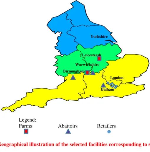
4.6. Finally, TOPSIS is applied as an aid for decision makers for selecting the final Pareto solution. Table 11 shows the ranking of solutions according to their closeness coefficient (closeness from the ideal solution and the furthermost from the nadir solution). As shown in Table 11, solution#4 revealed the highest closeness coefficient (ccp = 0.381474185). Thus, it is selected as a final solution to design the
resilient and green meat supply chain network since it leads to the best compromise of economic, green and resilience performance. Based on this solution, the
27
minimum total cost is 409,515; the minimum CO2 emissions is 304,000 and the
maximum value of resilience pillars (V-RALF) is 2.285. Also, this solution requires the establishment of two farms to supply livestock to three abattoirs as geographically illustrated in Fig.5. This solution is obtained via an allocation of ε1=
304,075 and ε2 = 2.285.
Table 5. Linguistic pairwise comparison among resilience pillars based on decision experts
Pillars Robustness Agility Leanness Flexibility
ADM
Robustness - 1/SMI EI EI
Agility SMI - VSI SMI
Leanness 1/VSI 1/ - 1/VSI
Flexibility EI 1/SMI VSI -
RDM1
Robustness - 1/VSI VSI 1/SMI
Agility VSI - EI EI
Leanness 1/VSI 1/EI - 1/EI
Flexibility SMI EI EI -
RDM2
Robustness - 1/VSI EI 1/WI
Agility VSI - EI EI
Leanness 1/EI 1/EI - 1/VSI
Flexibility WI EI VSI -
Table 6. Importance weights of resilience pillars obtained via fuzzy AHP
Decision Maker
Pillars (Importance Weight)
Robustness Agility Leanness Flexibility
ADM 0.196316 0.585745 0.042457 0.175482
28
Table 7. Evaluation of potential farms and abattoirs with respect to resilience pillars based on decision makers’ experts
Decision Maker and Locations
Pillars
Robustness Agility Leanness Flexibility
ADM f1 H VH M H f2 VH VH H VH f3 M H L H RDM1 a1 VH VH M H a2 M M L H a3 VH VH H VH a4 M H L H RDM2 a1 VH VH L VH a2 L M M M a3 VH VH M VH a4 M H M M
Table 8. Importance weights of farms and abattoirs with respect to resilience pillars obtained via the fuzzy technique
Locations
Pillars (Importance Weight)
GW Rank
Robustness Agility Leanness Flexibility
f1 0.65438 0.210868 0.14152 0.053407 0.343866 2 f2 0.84135 0.210868 0.19813 0.068666 0.383483 1 f3 0.46741 0.164008 0.08491 0.053407 0.272640 3 a1 0.39794 0.131638 0.10181 0.087664 0.269278 2 a2 0.22108 0.073132 0.06109 0.112711 0.214060 4 a3 0.39794 0.131638 0.14254 0.112711 0.298397 1 a4 0.22108 0.102385 0.06109 0.087664 0.218266 3 *GW = Global Weight
Table 9. Maximum and minimum values related to O1, O2 and O3
Objective functions Max Min
O1 501868 344703
O2 517847.785 180075.077
29
Table 10. Pareto optimal solutions obtained via the ε-constraint method
values Objective function solutions Opened Facilities # α-level
1
2 Min O1 Min O2 Min O3 Farms Abattoirs
1 0.1 211075 2 361348 211000 2 0 1 0 1 0 1 0 2 0.2 241075 2.095 370350 241075 2.095 0 1 0 1 0 1 0 3 0.3 271075 2.190 389550 268223 2.200 1 1 0 1 0 1 0 4 0.4 304075 2.285 409515 304000 2.285 1 1 0 1 0 1 1 5 0.5 337075 2.380 427626 335262 2.390 0 1 1 1 0 1 1 6 0.6 370075 2.475 446631 369998 2.482 1 1 0 1 0 1 1 7 0.7 404075 2.570 465843 404000 2.600 1 1 1 1 1 1 0 8 0.8 437075 2.655 470052 437005 2.655 1 1 0 1 1 1 1 9 0.9 490075 2.732 481118 488200 2.744 1 1 1 1 1 1 1 10 1 517847 2.790 492512 509121 2.790 1 1 1 1 1 1 1
Table 11. Membership degrees related to O1, O2 and O3
µ(O1) 0.97 0.83 0.77 0.62 0.75 0.59 0.39 0.28 0.15 0.066 µ(O2) 0.93 0.87 0.71 0.66 0.49 0.4 0.31 0.28 0.15 0.07 µ(O3) 0.09 0.18 0.25 0.32 0.4 0.51 0.68 0.78 0.8 0.91
Fig. 3. Trade-off solutions in relation to the three objectives. 200000 250000 300000 350000 400000 450000 500000 550000 350000 380000 410000 440000 470000 500000 CO 2 Total cost 1.8 2 2.2 2.4 2.6 2.8 3 350000 385000 420000 455000 490000 525000 V -RA L F Total cost 1.8 2 2.2 2.4 2.6 2.8 3 200000 250000 300000 350000 400000 450000 500000 550000 V -RA L F CO2
30
Figure 4. Pareto frontier among the three objectives.
Table 12. Ranking of Pareto solutions via TOPSIS
# ccp Rank 1 0.381371417 4 2 0.381388764 3 3 0.381412348 2 4 0.381474185 1 5 0.03238451 10 6 0.034367057 9 7 0.036469343 8 8 0.037900819 7 9 0.040307304 6 10 0.041510041 5
31
Figure 5. Geographical illustration of the selected facilities corresponding to solution#4.
5.2 Sensitivity analysis
A sensitivity analysis is performed to study the effects of changing the weight of resilience pillars on the weights of facilities. Eight different scenarios of weights are assigned to resilience pillars (see Eq. 3) related to farms and abattoirs. Tables 13 and 14 show the results related to the importance weights of farms and abattoirs, respectively. As shown in Tables 13 and 14, the sensitivity analysis reveals small variations in the importance weight of facilities. However, both farm 2 and abattoir 3 obtained the highest global weights for the eights scenarios of weights. This can be interpreted as the robustness of our implemented approach in finding the weight of facilities with respect to the resilience pillars. Finally, another sensitivity analysis is also conducted to investigate the effects of varying the weight of the three objectives (i.e., minimization of total cost and environmental impact and maximization of Value of resilience pillars) on the obtained ranking of Pareto solutions obtained by using TOPSIS. Six different combinations of weights are assigned to the three objectives in Eq. 50. Table 15 shows the obtained ranking of Pareto solutions for the six different combinations of weights. As shown in table 15, the sensitivity analysis reveals small variations in the ranking of Pareto solutions as solution#4 revealed the highest closeness coefficient value (ccp) in most runs. However,
Legend:
Farms Abattoirs Retailers
London Yorkshire Warwickshire Leicestersh ire Balham Birmingham
32
Pareto solutions are found to be more sensitive to the weight variation of the third objective (i.e., maximization of Value of resilience) compared to the weight of objectives one and two.
Table 13. Sensitivity analysis of weights of resilience pillars related to importance weights of farms
Weights of resilience pillars GW
R A L F f1 f2 f3 1 0.9 0.025 0.025 0.05 0.332550725 0.425946170 0.241503106 2 0.8 0.1 0.05 0.05 0.334550725 0.421755694 0.243693582 3 0.7 0.1 0.1 0.1 0.333101449 0.421797101 0.245101449 4 0.64 0.12 0.12 0.12 0.333055072 0.420442236 0.246502692 5 0.025 0.9 0.025 0.05 0.355884058 0.365946170 0.278169772 6 0.1 0.8 0.05 0.05 0.353217391 0.373755694 0.273026915 7 0.025 0.05 0.9 0.025 0.333942029 0.458496894 0.207561077 8 0.05 0.05 0.1 0.8 0.311478261 0.399138716 0.289383023
R =Robustness; A=Agility; L=Leanness; F=Flexibility
Table 14. Sensitivity analysis of weights of resilience pillars related to importance weights of abattoirs
Weights of resilience pillars GW
R A L F a1 a2 a3 a4 1 0.9 0.025 0.025 0.05 0.314667659 0.183110119 0.320570437 0.181651786 2 0.8 0.1 0.05 0.05 0.311969246 0.181919643 0.320649802 0.18546131 3 0.7 0.1 0.1 0.1 0.333101449 0.304652778 0.186458333 0.322013889 4 0.64 0.12 0.12 0.12 0.301297619 0.188035714 0.322130952 0.188535714 5 0.025 0.9 0.025 0.05 0.295917659 0.172693452 0.301820437 0.229568452 6 0.1 0.8 0.05 0.05 0.296969246 0.17358631 0.305649802 0.223794643 7 0.025 0.05 0.9 0.025 0.278504464 0.169828869 0.380066964 0.171599702 8 0.05 0.05 0.1 0.8 0.233849206 0.258928571 0.294960317 0.212261905 R =Robustness; A=Agility; L=Leanness; F=Flexibility