VTC Institutional Repository
VTC Institutional Repository
Staff Publications
Engineering
2019
Autonomous Vehicles: Autodriver Algorithm and Vehicle
Autonomous Vehicles: Autodriver Algorithm and Vehicle
Dynamics
Dynamics
Hormoz Marzbani
RMIT Univeristy, [email protected]
Hamid Khayyam
RMIT Univeristy
Ching Nok, Catter To
Hong Kong Institute of Vocational Education (Tsing Yi), Vocational Training Council, [email protected]
Đạ
i Võ Qu
ố
c
Reza N. Jazar
RMIT University
Follow this and additional works at: https://repository.vtc.edu.hk/ive-eng-sp
Part of the Mechanical Engineering Commons
Recommended Citation
Recommended Citation
Marzbani, H.,Khayyam, H.,To, C.,Quốc, Đ.,& Jazar, R. (2019). Autonomous Vehicles: Autodriver Algorithm and Vehicle Dynamics. IEEE Transactions on Vehicular Technology, 68 (4), 3201-3211. http://dx.doi.org/ 10.1109/TVT.2019.2895297
This Journal Article is brought to you for free and open access by the Engineering at VTC Institutional Repository. It has been accepted for inclusion in Staff Publications by an authorized administrator of VTC Institutional
Copyright (c) 2015 IEEE. Personal use of this material is permitted. However, permission to use this material for any other purposes must be obtained from the IEEE by sending a request to [email protected].
Abstract
—
A given road can be expressed mathematically in a global (or world) coordinate frame. Following the road can be substituted by following the loci of its curvature center and turning at the right circle of curvature. Considering that a vehicle in motion is always in turn about an instantaneous rotation center relative to the ground, an autonomous vehicle capable of following a given path by coinciding the rotation center of vehicle at every moment on the curvature center of the road could be designed. The dynamic reactions of the vehicle influence its path of motion and make its rotation center to depart from the desired path of the curvature center of the road. In this study the Autodriver algorithm control strategy to front-wheel-steering vehicles has been developed and a control loop is introduced to compensate the present errors generated by the differences of the desired locating on the road and the real position of the vehicle.keywords— Autonomous vehicle, Vehicle Control, Vehicle Dynamics, Road Curvature Center
I. INTRODUCTION
Autonomous vehicles have been a major focus of research in automotive engineering within recent decades [1]. One of the enormous technical challenges of autonomous vehicles is lateral controller for designing of dynamic path tracking, as a key component of the control system. A development method to achieve lateral control of autonomous vehicles is a steering control system [2-7]. The output of most of the controllers for lateral direction reported previously is the determination of the steering angle which is based on path planning approaches and by sensing state parameters of the vehicle. There are many mechanisms by which the optimal trajectories can be determined for steering mechanisms, using cost function optimization techniques. For steering control execution, the cost map method is used to calculate the optimal path. Cost maps enable fusing of the information collected using several sensors on the vehicle, allowing for a more universal and highly accurate assessment of reliability of the generated path. However, control method of autonomous vehicles which are based on steering angle result in inaccurate tracking with respect to position on the desired path, because as a vehicle moves in real-time, the steering wheel direction changes. A circular path with constant curvature is followed when the steering angle is fixed. In the case of varied steering angle, however, there will be a change in curvature. In this case, using a clothoid geometry function, the vehicle motion can be estimated. The curve used to transition from a straight road to a circular road or vice versa is called the clothoid, or Euler spiral. To avoid the challenges mentioned earlier, as an alternative steering angle based control, Broggi, et. al. [8] used a steering
1 Corresponding Author; RMIT University,
[email protected], +61 3 9925 6147
rate control approach. [9] Stated a driver steering model which analyzes vehicle test data subject to different driver steering scenarios during a standard double-lane-change movement by capturing key driver steering mechanisms. In this approach drivers control the steering rate in amount to their error with respect to the target angle which suggests implementation of a steering rate-based control, instead of the conventional steering angle control [9]. Bae et.al proposed a steering rate-based controller [10] in which at the planning stage, the curvature of the desired trajectory was determined before calculating the time derivative of the steering angle required and steering rate for accurate control. A linear “bicycle model” was used to model the lateral kinematics of the vehicle using the steering angle of both the front wheels [11]. Various other research efforts in this area have enhanced the design of roads intended to be used by autonomous vehicles [12-17]. Recent research have proposed to construct the intelligent transportation systems, variable smarter suspensions, steering systems, torque distribution, steering by wire, and vehicle dynamic modeling improvement on designing more safer and intelligent vehicles [18-21]. As an example a combination of GPS, sensory systems, mathematical and smart algorithms show to be the future answer to fully automated and driverless vehicles. Besides the technical aspects of autonomous vehicles, variety of studies are conducted about social impacts, regulations, human machine interfaces, and implementation methods of autonomous vehicles [22, 31, 32]. Most of the algorithms introduced for autonomous control of a vehicle have been introduced, rely on vision systems and sensory equipment in general and are quite functional for searching in unknown, structured environments. There exist other systems designed to guide a vehicle from a starting point or posture to a destination with a known posture by the use of smart decision making algorithms in conjunction with some sort of obstacle avoidance strategy. Controlling the vehicle’s position using GPS is also an alternative applicable method for some applications. The most suitable or easy to use methods for road vehicles are based on paths of motion which are previously mapped and planned. GPS can then be used to determine the best path to be taken by the vehicle [1]. However, roads are known and they can be well defined using mathematical equations in a coordinate frame attached to the ground called the global frame. Curvature center and curvature radius of such roads as well as all the other geometrical characteristics can be determined and employed for designing the required control system. A novel algorithm called Autodriver was introduced in 2010 which presented the theory mathematically and is used as the proof of concept for the current investigation [23]. The theory is also adopted,
Hormoz Marzbani
1, Hamid Khayyam,
Senior Member, IEEE,
Ching Nok TO,
Đại Võ Quốc and Reza N. Jazar
Autonomous Vehicles: Autodriver Algorithm
and Vehicle Dynamics
developed farther, and applied by other investigators [24, 25]. The original Autodriver algorithm manuscript [23] introduces the concept of replacement of given roads with the path of their curvature centers. Any moving vehicle on a road is continuously considered to be in a turn, near the curvature center of the road at any instant in time, which results in three points of importance: 1-road curvature center, or in other words the geometrical information of the road independent of the vehicles, 2- the rotation center found kinematical which is the intersection of the perpendicular line to the wheels of the vehicle; the kinematic rotation center is ideally a single point about which the vehicle tends to turn at no speed and 3-dynamic turning point or the real rotation center for the vehicle in motion. The location of the dynamic center of rotation is a dynamic properties function of the vehicle such as position of mass center, mass moments, tire-road interaction coefficients, steer angle, and vehicle velocity. The Autodriver algorithm is coinciding the dynamic center of rotation and the road curvature center at all times during the motion by adjusting steer angle and velocity of the vehicle. Although the use of autopilot algorithms in aircrafts, ships, spacecraft, or missiles have been happening for a while now, they are mostly not suitable for ground vehicles because of the interactions with the road and theoretically a one-dimensional road path constraint. Despite the ongoing investigation of method by picking the curvature center of the road to be the autonomous vehicle rotation center, there is still a gap. Most of the existing work do not take into account: to reduce or even eliminate the drivers’ tasks, as the main driver task or function is to keep steering to retain the vehicle on the road, to make a control strategy to remove error to follow a previously given path by just turning around the curvature center. Main contributions of this paper are as follows: (i) constructed a stochastic road geometry for the road curvature (bend) (ii) developed a new Autodriver algorithm for front-wheel-steering by redefining the mathematical theory, (iii) identify critical errors in highway (inter-city) travel for autonomous vehicles and (iv) developed a control strategy to eliminate errors for autonomous driving tasks. The paper is organized as follows. Section 2 describes the road geometry with respect to the vehicle. Section 3 presents the kinematic and dynamic vehicle rotation center for the management of energy consumption. Section 4 describes the dynamic rotation center. The autonomous control is presented in Section 5. Section 6 introduces some case study scenarios of the application of the algorithm. Finally, the concluding remarks are given in Section 7.
II. ROAD GEOMETRY
The three main factors include Driver, Environment, and Vehicle (DEV) are involved in energy management and vehicle performance. The modelling approach has become a vital tool for automotive engineers and mechanical researchers to reduce time consuming and improving efficiency of vehicle design. The modelling results have environmental benefits as well as significant cost saving. Among the factors that are involved in the vehicle system, the environment conditions such as road geometrical such as vertical curve (slope) and horizontal curve (bend) conditions are often unknown and uncertain during driving.
A. Horizontal Curve
A horizontal road can be assumed to be a number of straight lines and circular curves. Transition curve is the name chosen for the curves smoothly attaching straight lines to circles on the road. A curve of sufficient length is normally used whenever there is a change of direction in a road alignment in order to avoid the appearance of a sudden change in direction for vehicle travelling on the road.
The two major reasons for vehicle instability on the road are: ● Sliding: When a vehicle is traveling around a curve, a
lateral friction directly related to the square of the vehicle’s speed is developed at the tire-road interface. The force required maintaining a circular path eventually exceeds the force which can be developed by friction and super elevation, as speed is increased. ● Overturning: Often a heavy vehicle issue or in other
words vehicles with a high center of gravity. An overturning moment is formed by the forces acting on the vehicle which then cause rollovers for a vehicle in a turn.
B. Road Curvature Modeling
In order to produce credible vehicle on the road simulation, a realistic environmental modeling is necessary. The stochastic models proposed by [26, 27] are used for creating artificial environmental conditions for the present study.
C. Road Curvature Center
Consider a road to be expressed as a parametric curve in 3 dimensions
𝑥 = 𝑥(𝑠), 𝑦 = 𝑦(𝑠), 𝑧 = 𝑧(𝑠) (1)
where s is the distance traveled on the road measured from a point fixed on the road chosen to be the initial location of the vehicle.
𝑥
0= 𝑥(0), 𝑦
0= 𝑦(0), 𝑧
0= 𝑧(0)
(2)
Three important planes exist for any point on the road: the osculating plane, the perpendicular to the road plane, and the rectifying plane defined respectively as:
(𝑥 − 𝑥
0)
𝑑𝑥 𝑑𝑠+ (𝑦 − 𝑦
0)
𝑑𝑦 𝑑𝑠+ (𝑧 − 𝑧
0)
𝑑𝑧 𝑑𝑠= 0
(3)
(
𝑑𝑦𝑑𝑠 𝑑𝑑𝑠2𝑧2−
𝑑𝑧𝑑𝑠 𝑑𝑑𝑠2𝑦2) (𝑥 − 𝑥
0) + (
𝑑𝑧 𝑑𝑠 𝑑2𝑥 𝑑𝑠2−
𝑑𝑥 𝑑𝑠 𝑑2𝑧 𝑑𝑠2) (𝑦 −
𝑦
0) + (
𝑑𝑥 𝑑𝑠 𝑑2𝑦 𝑑𝑠2−
𝑑𝑦 𝑑𝑠 𝑑2𝑥 𝑑𝑠2) (𝑧 − 𝑧
0) = 0
(4)
(𝑥 − 𝑥
0)
𝑑2𝑥 𝑑𝑠2+ (𝑦 − 𝑦
0)
𝑑2𝑦 𝑑𝑠2+ (𝑧 − 𝑧
0)
𝑑2𝑧 𝑑𝑠2= 0
(5)The osculating plane includes the tangent line and point P which is the center of curvature of the road. The rectifying plane is vertical with respect to both osculating and normal planes [28]. The perpendicular plane is indicated by the tangential unit vector𝑢̂ = 𝑑𝑡 𝑟⁄𝑑𝑠
,
the osculating plane is identified by bi-vector 𝑢̂ = 𝑢𝑏 ̂ × 𝑢𝑡 ̂𝑛,
and the rectifying plane is identified by the normal unit vector𝑢
̂ = 𝑑
𝑛 2𝑟 𝑑𝑠
⁄
2.
Figure 1 depicts theroad center, radius of road curvature and the three plans at a point P of a road.
3
Figure 1. Osculating plane, curvature center and road’s radius of curvature at point P.
Curvature κ of a road at point P which has a curvature radius ρ can be calculated by 𝑘 = 1 𝑅𝑘= | 𝑑2𝑟 𝑑𝑠2| = |𝑣×𝑎| |𝑣|2 = √( 𝑑2𝑥 𝑑𝑠2) 2 + (𝑑2𝑦 𝑑𝑠2) 2 + (𝑑2𝑧 𝑑𝑠2) 2
(6) where
v
,
a , r
are the vehicle’s velocity, acceleration, and position vectors respectively. A vector can show the position of the center of curvature of a space curve 𝑟𝑐= 𝑅𝑘𝑢̂𝑛.These equations are significantly less difficult in the case of a planar road model. If a road with a given equation Y=f(X) is considered to exist in a global coordinate frame G, the radius of curvature
R
κof such a road
at any point X of the road is:𝑅
𝑘=
(1+𝑌′2)3⁄2 𝑌′′, 𝑌
′=
𝑑𝑌 𝑑𝑋, 𝑌
′′=
𝑑2𝑌 𝑑𝑋2(7)
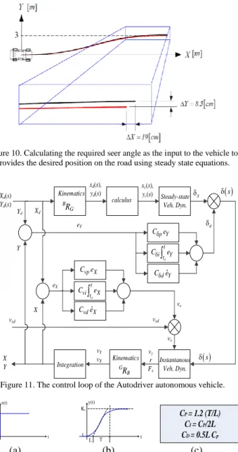
Figure 2(a) illustrates a road constructed by SMRG [27] used for this study, and Figure 2(b) shows an example of a two-dimensional road ( ) and its center of road. The arrows indicate the path of traveling along the road and its associated path of road curvature center. Figure 3 also depicts a three-dimensional road with the following parametric equation.
𝑥 = (𝑎 + 𝑏 sin 𝜃) cos 𝜃 𝑦 = (𝑎 + 𝑏 sin 𝜃) sin 𝜃
𝑧 = 𝑎 + 𝑏 sin 𝜃
𝑎 = 250𝑚 , 𝑏 = 200𝑚 (8)
where x and y are the coordinates of the location of the road presented in parametric format, a and b are magnification factors and θ is the heading angle of the road.
Substituting a road with its center of curvature helps road following by making the vehicle to always turn on the instantaneous curvature circle about the instantaneous curvature center. Straight motion of a vehicle is equal to a turn, about a point at infinite distance. This way, the vehicle will follow the given path if it turns about the road center at the correct distance of radius of curvature at any time.
(a)
(b)
Figure 2. (a) Constructed road direction by SMRG [27] method, (b) A two dimensional road and its road curvature center paths.
Figure 3. A three dimensional closed road and its curvature center path. The present study has been applied on many of the above mentioned roads and geometries. This was done to test the viability of the methods in different scenarios. The presented model in this document has been chosen to be a lane change maneuver though. This has been done to provide the readers with the solutions to one of the main activities required by an autonomous vehicle at the moment.
III. KINEMATIC ANALYSIS AND DYNAMIC VEHICLE ROTATION CENTER
The kinematic center of rotation for a front-wheel-steering car is on a line perpendicular to the rear wheels – in line with the extended line of the rear axle. The kinematic rotation center is at the intersection of lines which are perpendicular to the wheels which in an ideal case will intersect at a point at all times. The rotation kinematic center is theoretically the point that vehicle tends to turn but this will happen only at low velocities close to zero. When a front-wheel-steering vehicle is cruising at low speeds, the kinematic condition between its inner and outer wheels allowing them to turn without slipping on the ground
(slip-free) is expressed by (Ackerman condition)
𝑐𝑜𝑡𝛿
𝑜− 𝑐𝑜𝑡𝛿
𝑖=
𝑤𝑙
(9)
where,
δ
i andδ
o are the steer angles of the inner and outerwheels respectively. Track
(
w)
and wheelbase(
l)
are considered and also known as kinematic width and length of a vehicle [18]. The kinematic radius of rotation of such a vehicle, R, is the distance from the vehicle’s center of mass C and the kinematic center.𝑅 = √𝑎
22+ 𝑙
2𝑐𝑜𝑡
2𝛿
(10)
where
𝑎
2 is the longitudinal distance between rear axle and point C (location of the center of gravity), andδ
is the cot-average of the inner and outer steer angles.𝑐𝑜𝑡𝛿 =
𝑐𝑜𝑡𝛿𝑜+𝑐𝑜𝑡𝛿𝑖2
(11)
The angle
δ
is the equivalent steer angle which is used for any vehicle’s bicycle model having a wheelbasel
and radius of rotationR
.
Substituting an equivalent bicycle model of a vehicle is a standard and popular method in vehicle dynamics in order to significantly simplify the resulted mathematical equations.As soon as the vehicle moves, some side slip happens that makes the real location of the vehicle to deviate from the kinematic path of motion. The amount of deviation depends on the dynamic and geometric characteristics of the vehicle, steer angles, speed, and tire-road interaction properties. Inputting a constant value for velocity and steer angles of the vehicle would result in a steady state circular path of motion. The center of such a steady state circle is the actual or rotation dynamic center. To visualize this phenomena consider a vehicle that is supposed to turn around the origin of a global coordinate frame
G
(
X,Y
)
on a circle with radiusR=100
m.
A vehicle starts at a location on theX
-
axis while its longitudinal localx
-
axis is atY
=
100
m
parallel to theY
-
axis and its rear axle is on theX
-
axis.
At the starting instant, the kinematic rotation center of the vehicle is set to be on the origin. Assuming a non-zero constant velocity, the vehicle will slip out laterally such that a larger circle will be tracked about its dynamic center which is illustrated in Figure 4. The mathematical analysis of kinematic rotation center of four-wheel steering vehicles provides a set of similar equations involving more parameters that have been studied before [29]. v cc X 100 50 Dynamic path Road Path of kinematic center Dynamic center Road curvature center -50 -100 100 Y x y Gd
Figure 4. The dynamics of an understeer vehicle makes it go out of the static designed path. The dynamic curvature center deviates from the road curvature
center when steering angles kept at the required static values to turn about road curvature (not in scale).
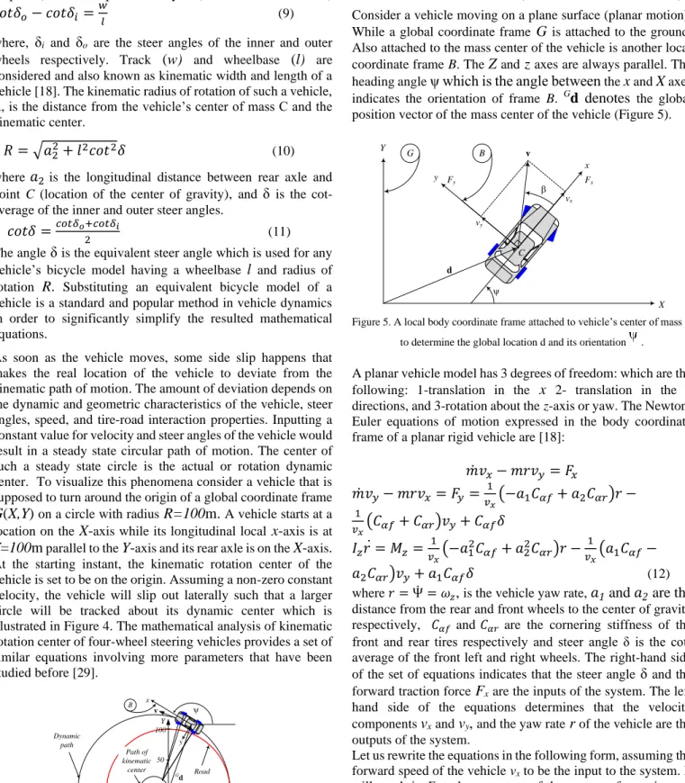
IV. VEHICLE DYNAMICS (HIGH VELOCITY MANEUVERS) Consider a vehicle moving on a plane surface (planar motion). While a global coordinate frame
G
is attached to the ground. Also attached to the mass center of the vehicle is another local coordinate frame B. TheZ
andz
axes are always parallel. The heading angleψ which is the angle between
thex
andX
axes indicates the orientation of frame B. Gd
denotes
the global position vector of the mass center of the vehicle (Figure 5).X Y C x y F x Fy v vx vy d B G
Figure 5. A local body coordinate frame attached to vehicle’s center of mass C to determine the global location d and its orientation .
A planar vehicle model has 3 degrees of freedom: which are the following: 1-translation in the
x
2- translation in they
directions, and 3-rotation about thez-axis or yaw. The Newton-Euler equations of motion expressed in the body coordinate frame of a planar rigid vehicle are [18]:
𝑚̇𝑣
𝑥− 𝑚𝑟𝑣
𝑦= 𝐹
𝑥𝑚̇𝑣
𝑦− 𝑚𝑟𝑣
𝑥= 𝐹
𝑦=
1 𝑣𝑥(−𝑎
1𝐶
𝛼𝑓+ 𝑎
2𝐶
𝛼𝑟)𝑟 −
1 𝑣𝑥(𝐶
𝛼𝑓+ 𝐶
𝛼𝑟)𝑣
𝑦+ 𝐶
𝛼𝑓𝛿
𝐼
𝑧𝑟 =
̇
𝑀
𝑧=
1 𝑣𝑥(−𝑎
1 2𝐶
𝛼𝑓+ 𝑎
22𝐶
𝛼𝑟)𝑟 −
1 𝑣𝑥(𝑎
1𝐶
𝛼𝑓−
𝑎
2𝐶
𝛼𝑟)𝑣
𝑦+ 𝑎
1𝐶
𝛼𝑓𝛿
(12)
where 𝑟 = Ψ̇ = 𝜔𝑧
,
is the vehicle yaw rate,𝑎
1and
𝑎
2are the
distance from the rear and front wheels to the center of gravity respectively, 𝐶𝛼𝑓 and 𝐶𝛼𝑟 are the cornering stiffness of the front and rear tires respectively and steer angle δ is the cot-average of the front left and right wheels. The right-hand side of the set of equations indicates that the steer angleδ
and the forward traction forceF
xare the inputs of the system. The lefthand side of the equations determines that the velocity components
v
xandv
y,
and the yaw rater
of the vehicle are theoutputs of the system.
Let us rewrite the equations in the following form, assuming the forward speed of the vehicle vx to be the input to the system. It
will result in Fx to be an output of the system of equations of
5
𝑣
𝑥=
𝐹
𝑥𝑚
+ 𝑟𝑣
𝑦̇
𝑣
𝑦=
1
𝑚𝑣
𝑥(−𝑎
1𝐶
𝛼𝑓+ 𝑎
2𝐶
𝛼𝑟)𝑟 −
1
𝑚𝑣
𝑥(𝐶
𝛼𝑓+ 𝐶
𝛼𝑟)𝑣
𝑦+
1
𝑚
𝐶
𝛼𝑓𝛿 − 𝑟𝑣
𝑥̇
𝑟̇ =
1 𝐼𝑧𝑣𝑥(−𝑎
1 2𝐶
𝛼𝑓− 𝑎
22𝐶
𝛼𝑟)𝑟 −
1 𝐼𝑧𝑣𝑥(𝑎
1𝐶
𝛼𝑓−
𝑎
2𝐶
𝛼𝑟)𝑣
𝑦+
1 𝐼𝑧𝑎
1𝐶
𝛼𝑓𝛿
(13) The vehicle is assumed to move with constant velocity for the sake of simplifying the equations.
𝑣
𝑥= 𝑐𝑜𝑛𝑠𝑡𝑎𝑛𝑡
(14)
This will cause the steer angles of the vehicle to be the only dynamic system input. Therefore, the two outputs of the system will be the lateral speed
v
y,
yaw rater.
Traction forceF
xisanother output which according to the first equation will be determined by the velocity and the solutions of the equations. Having the function of the steering angles and starting from an initial condition for
v
y(0)
andr(0)
,
will enable thedetermination
of
v
y(lateral velocity)andr
(yaw rate)in futuretimes. Integrating
v
x,
v
yandr
,
results in the body and global(or world) coordinate representations of the position and the vehicle orientation.
Integrating the yaw rate of the vehicle will determine the heading angle or orientation
Ψ = ∫ 𝑟𝑑𝑡
0𝑡(15)
and now by multiplying the rotation transformation matrixG
R
B, the velocity vector of the vehicle in the global frame can be determined
.
𝑣
𝑐 𝐺= 𝑅
𝐵 𝐺𝑣
𝑐 𝐵[
𝑣
𝑣
𝑋 𝑌] = [
𝑐𝑜𝑠Ψ −𝑠𝑖𝑛Ψ 0
𝑠𝑖𝑛Ψ
𝑐𝑜𝑠Ψ
0
0
0
1
] [
𝑣
𝑣
𝑥 𝑦]
(16)
Integrating components of velocity expressed in the global frame and summed with the present location of the mass center will give the present location of the vehicle.
𝑑
𝐺= 𝑑
0+
𝐺∫ 𝑣
𝐺𝑑𝑡
[
𝑋
𝑌
] = [
𝑋
0𝑌
0] + [
∫ (𝑣
𝑥cos 𝜓 − 𝑣
𝑦sin 𝜓)𝑑𝑡
𝑡 0∫ (𝑣
𝑥sin 𝜓 + 𝑣
𝑦cos 𝜓)𝑑𝑡
𝑡 0]
(17)where Xo and Yo are the coordinates of the initial location which are assumed to be given values.
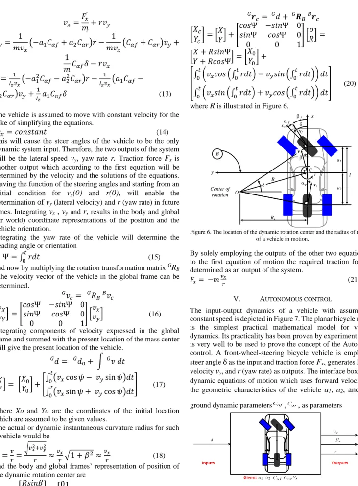
The actual or dynamic instantaneous curvature radius for such a vehicle would be
𝑅 =
𝑣 𝑟=
√𝑣𝑥2+𝑣𝑦2 𝑟≈
𝑣𝑥 𝑟√1 + 𝛽
2≈
𝑣𝑥 𝑟 (18)and the body and global frames’ representation of position of the dynamic rotation center are
𝒓
𝑐= [
𝑅𝑠𝑖𝑛𝛽
𝑅𝑐𝑜𝑠𝛽
] ≈ [
0
𝑅
]
𝐵(19)
𝒓
𝑐=
𝐺 𝐺𝑑
+ 𝑹
𝐵 𝐺𝒓
𝑐 𝐵[
𝑋
𝑌
𝑐 𝑐] = [
𝑋
𝑌
] + [
𝑐𝑜𝑠Ψ −𝑠𝑖𝑛Ψ 0
𝑠𝑖𝑛Ψ
𝑐𝑜𝑠Ψ
0
0
0
1
] [
𝑅
𝑜
] =
[
𝑋 + 𝑅𝑠𝑖𝑛Ψ
𝑌 + 𝑅𝑐𝑜𝑠Ψ
] = [
𝑋
0𝑌
0] +
[
∫ (𝑣
𝑥𝑐𝑜𝑠 (∫ 𝑟𝑑𝑡
𝑡 0) − 𝑣
𝑦𝑠𝑖𝑛 (∫ 𝑟𝑑𝑡
𝑡 0)) 𝑑𝑡
𝑡 0∫ (𝑣
𝑥𝑠𝑖𝑛 (∫ 𝑟𝑑𝑡
𝑡 0) + 𝑣
𝑦𝑐𝑜𝑠 (∫ 𝑟𝑑𝑡
𝑡 0)) 𝑑𝑡
𝑡 0]
(20) where
R
is illustrated in Figure 6.x y O l R R1 C a2 r a1 vr Center of rotation f f r vf v xw B
Figure 6. The location of the dynamic rotation center and the radius of rotation of a vehicle in motion.
By solely employing the outputs of the other two equations in to the first equation of motion the required traction force is determined as an output of the system.
𝐹𝑥= −𝑚
𝑣𝑥
𝑟
(21)
V. AUTONOMOUS CONTROL
The input-output dynamics of a vehicle with assuming a constant speed is depicted in Figure 7. The planar bicycle model is the simplest practical mathematical model for vehicle dynamics. Its practicality has been proven by experiment and it is very well to be used to prove the concept of the Autodriver control. A front-wheel-steering bicycle vehicle is employed: steer angle
δ
as the input and traction forceF
x,, generates lateralvelocity
v
y,
andr
(yaw rate)as outputs. The interface box is thedynamic equations of motion which uses forward velocity
v
x,the geometric characteristics of the vehicle
a
1,
a
2, and
tire-ground dynamic parameters
,
,
as parametersFigure 7. Input-output relationship in vehicle dynamics using planar bicycle model.
The outputs of the dynamic equations are time rate of kinematic variables in body coordinate frame. Transforming them to the global coordinate frame followed by integration, which determines the vehicle’s actual orientation and location on the ground coordinate frame. This step is illustrated in Figure 8(a). The result would be an actual location of the vehicle on the road to be compared with the desired location.
Figure 8 (a). Determination of the global position of a vehicle. To control the vehicle, we must solve an inverse dynamic problem and determine speed
v
x and steer angleδ
required
such that the actual vehicle position matches with the desired position on the road. Consider Figure 8(b) that shows a loop starting with a desired location on the road, X,Y,Z. The mentioned position coordinates will then be fed back to the set of integrations and kinematic transformation mentioned earlier so that the associated kinematics variables
of the vehicle
under study
r
,
andvy would be determined.
These variables, which are typically outputs of the vehicle dynamics, must be fed back to the vehicle’s dynamic equation box theoretically to determine the required steering angle inputδ
.
If this steer angleδ
was the correct value then feeding it into the box (dynamic equations) would locate the vehicle in the correct position and the real X,Y,Z would be the same as the desired one on the road. However, feeding the kinematic variablesr
,
andv
yinto the box(dynamic equation) in order to determine the required input
δ
is not a straightforward step and will not work properly. This is shown by the red box in Figure 8(b) to express the idea that there is not an easy way to determine the requirements.Figure 8(b). Ideal reverse dynamic to locate a vehicle at a desired position on the road. Reverse calculating (The box in red) the steer angle δ is not
straightforward
To solve reverse dynamics differential equations there are several numerical and approximation methods. The shooting method is the usual numerical method that might be a solution of the blocked box in Figure 8(b), however this method cannot be applied to an on-time control system. As a result we need to
introduce a quick method to calculate
δ
. [21]
and [30] investigated the transient responses of vehicles compared to their steady state responses. These studies show that under normal conditions, the vehicle’s transient response is very close to their steady state behavior or in other words that the vehicles are lazy. The same set of equations introduced earlier govern the steady state conditions of a vehicles. The major difference is that all time derivative operators is the equation are set to zero. This results in a set of algebraic equations which gives the steady state steer angleδ
ss.
0 =
𝐹
𝑥𝑚
+ 𝑟𝑣
𝑦̇
0 =
1
𝑚𝑣
𝑥(−𝑎
1𝐶
𝛼𝑓+ 𝑎
2𝐶
𝛼𝑟)𝑟 −
1
𝑚𝑣
𝑥(𝐶
𝛼𝑓+ 𝐶
𝛼𝑟)𝑣
𝑦+
1
𝑚
𝐶
𝛼𝑓𝛿 − 𝑟𝑣
𝑥̇
0 =
1 𝐼𝑧𝑣𝑥(−𝑎
1 2𝐶
𝛼𝑓− 𝑎
22𝐶
𝛼𝑟)𝑟 −
1 𝐼𝑧𝑣𝑥(𝑎
1𝐶
𝛼𝑓−
𝑎
2𝐶
𝛼𝑟)𝑣
𝑦+
1 𝐼𝑧𝑎
1𝐶
𝛼𝑓𝛿
(22)
Therefore, the blocked square with the set of steady state algebraic equations is substituted. This enables the estimation of the steer angle which generates the required
v
yand
r
thatthey are all at their steady state condition as illustrated in Figure 9. The calculated steer angle is used as input to the set of transient equations of motion to calculate instant values of
v
yand
r
associated with the scenario under investigation.
These variables will be used to calculate the actual road position of the vehicle. However, due to the approximated value of the steer angle, the coordinates of the vehicle on the ground would be potentially different than the desired values. The actual variables should be compared with the desired values to close the control loop and generate control strategy to compensate the errors.
There would be potential differences between
X
d, X
, which are
the desired and actual locations on the
X
axis respectively
and
Y
d, Y
which are the desired and actual locations on the
Y
axis respectively
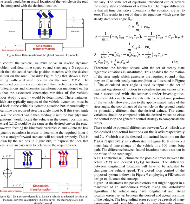
as is illustrated in Figure 10. It shows a 3 meter lateral lane change of the vehicle in a 100 meter long path. The difference between lateral locations needs a set-out in the value of the steer angel.A PID controller will eliminate the possible errors between the actual (X,Y) and desired (Xd,Yd) locations. The difference
between longitudinal locations will have to be adjusted by changing the vehicle speed. The closed loop control of the proposed system is shown in Figure 9 employing a PID control design to illustrate the concept.
Figure 10 illustrates the possible errors that might happen in a maneuver of an autonomous vehicle using the Autodriver algorithm. The vehicle may have longitudinal and lateral location errors, eX, eY, between the desired and actual positions
of the vehicle. The longitudinal error eX may be a result of many
parameters and variables such as aerodynamic forces, estimation of the tire and road characteristics, etc. However, it can be compensated by adjusting forward velocity of the vehicle using a controller on the longitudinal error signal. Similarly, the lateral position error eY, also may be a result of
7
of the road, misalignment of the wheels, etc. The lateral position error can be compensated by adjusting steer angle of the vehicle.
Figure 11 illustrates the overall control system and the loop starting with the desired global coordinates of the vehicle Xd(s),
Yd(s). These coordinates are functions of a parameter, say,
which varies when the distance vehicle moves on the road. The desired global (or world) coordinates will be transformed to the vehicle body coordinate frame. As a result, the road equation will be defined in the body coordinate to be used to calculate the loci of the road curvature center in the body coordinate in which the actual instant center of rotation of the vehicle will be calculated to compare. Then, the steady state equations of motion of the vehicle will provide an estimate for the required steer angle to turn the vehicle about the road curvature center at the current location of the vehicle. The estimated steer angle is one of the two required input set of (
δ
, vx) to feed theinstantaneous dynamic equations of motion of the vehicle. The output of the dynamic equations of motion are the lateral velocity vy, traction force Fx and yaw rate r. These outputs are
all calculated in the body coordinate frame. A backward transformation will provide us with their values in the global coordinate frame. Integrating velocity components and the yaw rate of the vehicle determines the position and orientation of the vehicle on the road, X,Y. At this stage the system needs to compare the real position of the vehicle with the desired one. The differences will generate the error signals to be fed into the PID controller and provide adjusting signals to the steer angle and forward velocity.
A. PID Tuning
The optimal values of the three PID gains can be tuned using several methods (i) off-line (practical) such as: 1- Ziegler-Nichols (ZN), 2- Cohen-Coon (CC), 3- Chien-Hrones-Reswick (CHR), 4- ITAE Tuning and (ii) on-line (intelligent) such as : 1- Neural Network Tuner (NNT), 2- Fuzzy Logic (FL), 3- Genetic Algorithm [31-33]. PID controllers tuned by ZN method are commonly used in automotive industry [32, 33]. Based on the values L and T (see Figure. 12 (a) and (b)), ZN finds the first setting of the controller. For aperiodic responses, the PID gains are tuned according to Figure. 12(c).
Figure 9. In the simplest dynamic model of planar vehicle and planar road.
Figure 10. Calculating the required seer angle as the input to the vehicle to provides the desired position on the road using steady state equations.
Xd(s) Yd(s) BR G calculus xd(s), yd(s) xc(s), yc(s) Steady-state Veh. Dyn. s e Instantanous Veh. Dyn. ( )s vy r Fx Kinematics vY vX Integration X Y G RB Kinematics Yd Y eY p Y C e ( )s vx vxd vp X C e X Xd eX ve vxd 0 t vit X C
e vd X C e 0 t it Y C
e d Y C eFigure 11. The control loop of the Autodriver autonomous vehicle.
t 1 x(t) t t Ks T L y(t) CP = 1.2 (T/L) CI = CP/2L CD = 0.5L Cp (a) (b) (c) Figure 12 (a) Test signal, (b) Unit-step response, and (c) ZN tuning.
VI. CASE STUDY SCENARIOS A. Constant velocity
Consider a vehicle with the following characteristics at a constant speed of
v
x=20
m/s
that is supposed to turn on a flatcircle of
R=100
m.
𝐶𝑓= 57000 𝑁 𝑟𝑎𝑑⁄ , 𝐶𝑟= 52000 𝑁 𝑟𝑎𝑑⁄
𝑚 = 900 𝑘𝑔, 𝐼𝑧= 1200 𝑘𝑔𝑚2
𝑎1= 0.91 𝑚, 𝑎2= 1.64 𝑚
(23) The same analysis was repeated with more complicated nonlinear inputs to the system to evaluate algorithm’s capability in different scenarios.
The proposed PID controller gains using ZN method are set to an estimated below value (see Eq. (24)) of
and applied to the
constant velocity
case.
[𝐶𝑃,𝐶𝐷, 𝐶𝐼,] = [0.12,0.075,0.031]
(24)
The path after the application of the controller is labeled
as exact compared to the Autodriver algorithm resulted
path labeled approximate in Figure 13. The differences in
the case of constant velocity and steering are small and
hard to see in Figure 13.
Figure 13. Applying the Autodrive autonomous control on a circular path motion.
B. Nonlinear varying steering
The study investigated different nonlinearities introduced to the system. The first example was done by keeping the velocity constant but changing the steering angle according to the following equation and result is in Figure 14.
𝛿 = 𝛿0(𝐻(𝑡 − 𝑡0) + 𝑠𝑖𝑛2(
𝑡
2𝑡0⁄𝜋) 𝐻(𝑡0− 𝑡)) (25)
Figure 14 - Nonlinear steering input to the Autodriver algorithm where 𝐻(𝑡 − 𝑡0)is the Heaviside function and 𝑡0= 1𝑠, is the response time.
The resultant path of motion with constant velocity and nonlinear varying steering is illustrated in Figure 15. The proposed PID controller gains tuned using ZN method are set to an estimated below value (see Eq. (26)) of
and applied to
constant velocity and nonlinear varying steering case
scenario.
[𝐶𝑃,𝐶𝐷, 𝐶𝐼,] = [0.2,0.09,0.04]
(26)
The comparison of resulted path of motion after and before application of PID controller on the constant velocity with variable steering case shown in Figure 16.
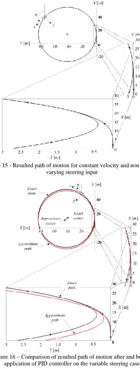
Figure 15 - Resulted path of motion for constant velocity and non linearly varying steering input
Figure 16 – Comparison of resulted path of motion after and before application of PID controller on the variable steering case C. Nonlinear variable velocity
For a second nonlinear test a variable velocity was used while the steering input was kept constant during the motion of the vehicle. The velocity was changed according to the below Equation.
𝑣𝑥=
20
𝑡0𝑡 𝐻(𝑡0− 𝑡) + 20 𝐻(𝑡 − 𝑡0) 𝑚 𝑠⁄ (27)
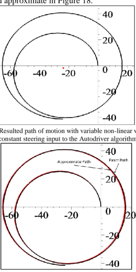
While the steering angle was kept at 0.1 𝑟𝑎𝑑/𝑠𝑒𝑐 during the motion. The resultant path of motion is illustrated in Figure 17. The proposed PID controller gains tuned using ZN method are set to an estimated below value of
and applied to nonlinear
variable velocity case scenario.
9
However, determination of the optimal gain values, considering variable gains, as well as making the control strategy more complicated are due for further future study. Application of the above mentioned controller resulted in reducing the errors significantly. The path after the application of the controller is labeled as exact compared to the Autodriver algorithm resulted path labeled approximate in Figure 18.
Figure 17- Resulted path of motion with variable non-linear velocity and constant steering input to the Autodriver algorithm
Figure 18 - Comparison of resulted paths of motion after and before application of the PID controller on the variable velocity case
VII. CONCLUSION
A vehicle with automatic steering is assumed to be driven on a given road. A function in the global coordinate frame is used to express the road together with another local coordinate frame attached to the center of mass of the vehicle. The curvature center of the road is then determined in the coordinates of the vehicle which is supposedly the vehicle’s rotation center too. Steering angle of the wheels may be adjusted in a way that the vehicle’s kinematic center of rotation and the road’s curvature center coincide using the kinematic steering conditions. This will enable the vehicle to follow the road only at extremely low speeds. However, the actual point that the vehicle is turning about when the vehicle speeds up would be different due to dynamic behaviors of the vehicle. It is possible to find out and calculate the dynamic center of rotation of a vehicle by solving the vehicle’s equations of motion which are a set of coupled ordinary differential equations. A feedback signal can be used together with an analysis of the differences between the three centers in order to add two correction terms to the steer angles or the traction force such that the dynamic rotation center and curvature center of the road coincide with each other. At the time the vehicle is dynamically turning around center of
curvature of the road, the kinematic center of rotation will move on a steering circle about the dynamic turning center.
This study presents the application of Autodriver algorithm for autonomous vehicles [12]. We believe that 4 wheel steering systems are a better choice for vehicle dynamically. The initial concept was based on these systems as a result. A step was taken to make the algorithm more practical which was generation of the algorithm for front wheel steering vehicles. The main objective when a vehicle is trying to follow a given path is to adjust the center of rotation of the vehicle so that it coincides with center of curvature of the road. The dynamic behavior of vehicles has other ideas. It results in the vehicle to slip on the ground. The act of slipping then causes the vehicle to deviate from the expected path of motion by the given steer angle and velocity. This is because of the existence of many factors most importantly sideslip of the vehicle. The differential equations of motion of the vehicle will need to be solved backwards, in order to find the actual path of motion. This not being possible initiated the investigation for alternative methods. The result was called “Steady-State Dynamic Steering” which is gained by the use of the steady-state responses or more specifically the curvature response of the vehicle in order to find the dynamic response of a vehicle. This method is a simple method of finding dynamic responses of a vehicle without having to solve the differential equations of motion within an acceptable engineering range.
The errors have been highlighted in comparison with the exact solutions are very small in different scenarios tested [24]. The suggested feedback control system will be able to prevent these small variations in the final results which were not an objective for the present study.
REFERENCES
[1] R. Bishop, Intelligent Vehicle Technology and Trend. Norwood, MA: Artech House, 2005.
[2] M. A. Sotelo, "Lateral Control Strategy for Autonomous Steering of Ackerman-like Vehicles," Robotics and Autonomous Systems, vol. 45, pp. p223-233, 2003.
[3] J. M. Snider, "Automatic Steering Methods for Autonomous Automobile Path Tracking," Carnegie Mellon University, Pittsburgh2009.
[4] V. Milanés, J. Pérez, E. Onieva, C. González, and T. de Pedro, "Lateral power controller for unmanned vehicles," Elect. Rev., vol. 86, pp. 207-211, 2010.
[5] J. Pérez, V. Milanés, and E. Onieva, "Cascade Architecture for Lateral Control in Autonomous Vehicles," IEEE Tr. on ITS, vol. 12, pp. 73-82, 2011.
[6] J. W. Lee and B. Litkouhi, "A Unified Framework of the Automated Lane Centering/Changing Control for Motion Smoothness Adaptation," presented at the International IEEE Conference on Intelligent Transportation Systems, Anchorage, Alaska, 2012. [7] M. H. Lee, K. Lee, S, H. G. Park, Y. C. Cha, J. D. Kim, B. Kim, et
al., "Lateral Controller Design for an Unmanned Vehicle via Kalman Filtering," International Journal of Automotive
Technology, vol. 13, pp. 801-807, 2012.
[8] A. Broggi, P. Medici, E. Cardarelli, P. Cerri, and A. Giacomazzo, "Development of the control system for the VisLab Intercontinental Autonomous Challenge," presented at the International IEEE Annual Conference on Intelligent Transportation Systems, , Madeira Island, 2010.
[9] H. Tan and J. Huang, "Experimental development of a new target and control driver steering model based on DLC test data," IEEE Tr.
on ITS, vol. 13, pp. 375-384, 2012.
[10] I. Bae , J. Hyo Kim, and S. Kim, "Steering Rate Controller based on Curvature of Path for Autonomous Driving Vehicles," presented at the IEEE Intelligent Vehicles Symposium (IV), Australia,, 2013.
[11] R. Rajamani, Lateral Vehicle Dynamics Springer, 2006.
[12] M. Elbanhawi, M. Simic, and R. N. Jazar, "Autonomous Robots Path Planning: An Adaptive Roadmap Approach," Applied
Mechanics and Materials., vol. 373, pp. 246-254, 2013.
[13] M. Elbanhawi, M. Simic, and R. N. Jazar, "Continuous-Curvature Bounded Path Planning Using Parametric Splines," Frontiers in
Artificial Intelligence and Applications, vol. 262, pp. 513-522, 2014.
[14] H. Marzbani, M. Simic, M. Fard, and R. N. Jazar, "Better Road Design for Autonomous Vehicles Using Clothoids," Intelligent
Interactive Multimedia Systems and Services, vol. 40, pp. 265-278,
2015.
[15] V. D.Q., M. H., F. M., and R. N. Jazar, "A Novel Kinematic Model of a Steerable Tire for Examining Kingpin Moment during Low-Speed-Large-Steering-Angle Cornering," SAE International
Journal of Passenger Cars-Mechanical Systems vol. 10, 2016.
[16] V. D.Q., M. H., F. M., and R. N. Jazar, "Variable caster steering in vehicle dynamics " Proceedings of the Institution of Mechanical
Engineers, Part D: Journal of Automobile Engineering 2017.
[17] M. Guiggiani, The Science of Vehicle Dynamics: Handling,
Braking, and Ride of Road and Race Cars: Springer, 2014.
[18] Fu C., H. R., B.-H. A., and R. N. Jazar, "Electric Vehicle Side-Slip Control via Electronic Differential," International Journal of
Journal of Vehicle Autonomous Systems, vol. 6, pp. 108-132, 2014.
[19] Marzbani H., Harithuddin S., Simic M., Fard M., and R. N. Jazar, "Steady-State Dynamic Steering," Frontiers in Artificial
Intelligence and Applications, vol. 262, pp. 493-504, 2014.
[20] P. K. Agarwal and H. Wang, " Approximation algorithms for curvature-constrained shortest paths," SIAM J. Comput. , vol. 30, pp. 1739-1772, 1996.
[21] Marzbani H., Vo DQ., Khazaei A., Fard M., and R. N. Jazar, "Transient and steady-state rotation centre of vehicle dynamics,"
International Journal of Nonlinear Dynamics and Control, vol. 1,
pp. 97-113, 2017.
[22] Lari A. and O. I. Douma F., " Self-Driving Vehicles and Policy Implications: Current Status of Autonomous Vehicle Development and Minnesota Policy Implications," Minnesota Journal of Law,
Science & Technology, vol. 16, 2015.
[23] R. N. Jazar, "Mathematical Theory of Autodriver for Autonomous Vehicles " Journal of Vibration and Control vol. 16, pp. 253-279, 2010.
[24] Marzbani H., "Application of the Mathematical Autodriver Algorithm for Autonomous Vehicles ", School of Engineering, RMIT University Melbourne Australia, 2014.
[25] A. Bourmistrova, M. Simic, R. Hoseinnezhad, and R. N. Jazar, " Autodriver Algorithm," Journal of Systemics, Cybernetics and
Informatics, vol. 9, pp. 55-56, 2011.
[26] H. Khayyam, A. Kouzani, H. Hamid Abdi, and S. Nahavandi, "Modeling of Highway Heights for Vehicle Modeling and Simulation," in ASME 2009 International Design Engineering Technical Conferences and Computers and Information in
Engineering Conference, 2009, pp. 365-369.
[27] H. Khayyam, "Stochastic Models of Road Geometry and Wind Condition for Vehicle Energy Management and Control," IEEE
Transaction on Vehicular Technology, vol. 62, pp. 61-68, 2012.
[28] R. N. Jazar, Advanced Dynamics: Rigid Body, Multibody, and
Aerospace Applications: Wiley, New York 2011.
[29] H. Marzbani, S. Harithuddin, M. Simic, M. Fard, and R. N. Jazar, "Four wheel steering advantagous for the Autodriver algorithm "
Frontiers in Artificial Intelligence and Applications, vol. 262, pp.
505-512, 2014.
[30] R. N. Jazar, Vehicle Dynamics: Theory and Application. New York: Springer, 2018.
[31] Hamid Khayyam, Abbas Z Kouzani, Eric J Hu, Saeid Nahavandi, “Coordinated energy management of vehicle air conditioning system” Applied thermal engineering, vol 31, pp 750-764, 2011. [32] Sihai Song, Wenjian Cai, Ya-Gang Wang, “Auto-tuning of cascade
control systems” ISA Transactions, vol 42, pp 63–72, 2003. [33] J. M. S. Ribeiro, M. F. Santos, M. J. Carmo, M. F. Silva “Comparison
of PID Controller Tuning Methods: Analytical/Classical Techniques versus Optimization Algorithms” 18th International Carpathian Control Conference (ICCC), pp 533-538, 2017.
Hormoz Marzbani received his PhD in Mechanical
Engineering in 2015 and is working as lecturer in RMIT University, Melbourne, Australia since. His main research interests are in the field of Dynamics, Vibration, Vehicle Dynamics and autonomous systems.
The autodriver algorithm which is a novel methematical theory for autonomous driving of the cars consideing the vehicle dynamics, constraints and methemtics of the road ahead is his majro field of study and contribution
Hamid Khayyam (SM’13) received the B.Sc
(Honours) degree from the University of Isfahan, the M.Sc. degree from the Iran University of Science and Technology, and the Ph.D. degree in Mechanical (Mechatronics) Engineering from Deakin University, Australia. He has worked in automation and productivity of process lines in various industrial companies for more than 10 years.
In his previous position he was leading the efforts on modelling and optimisation of energy systems in the carbon fibre production line at Deakin University. Dr. Khayyam has published more than 82 peer reviewed journal papers, conference papers and book chapters. Dr. Khayyam's research activities focus on system identification, modelling, control, simulation-based optimization of complex energy systems, applications of artificial intelligence techniques and optimization methods for engineering. He is currently senior lecturer at RMIT University in Australia.
Ching Nok TO, received the B.Eng (Hons.) & M.Eng. degrees in Mechanical from the Hong Kong Polytechnic University, in 2003.
He is currently a Lecturer with Department of Engineering, the Institute of Vocational Education (Tsing Yi), Vocational Training Council.
His research interests include Vehicle Dynamics, Autonomous Vehicles and Autodriver Algorithm.
Đại Võ Quốc received the Ph.D degree in Mechanical & Manufacturing Engineering from RMIT University, Melbourne, Australia, in 2017. He is currently a lecturer in Faculty of Vehicle and Energy Engineering, Le Quy Don Technical University, Vietnam.
His research interests include kinematics, dynamics of vehicle systems, dynamics, ride, handling and stability of vehicles; and caster steering theory. He has published many papers, book chapters, and technical papers in the field.
Reza N. Jazar is a professor of Mechanical Engineering and Applied Mathematics and is the Head of Mechanical and Automotive Engineering at the School of Engineering, RMIT University, Melbourne, Australia. He has several years of work experience in Automotive Engineering, as well as Academic experiences in several universities all around the world.
He is the author of more than 200 scientific papers and monographs, and the author of several famous technical and textbooks including:
Nonlinear Approaches in Engineering Applications, co-author, Springer, New York, 2012, 2014, 2015, 2016, 2018, 2019.
Vehicle Dynamics: Theory and Application, Second Edition, Springer, New York, 2009,2014, 2017.
Advanced Vibrations: A Modern Approach, Springer, New York, 2013. Advanced Dynamics, Rigid Body, Multibody, and Aerospace Applications, Wiley, N Y, 2011.
Professor Jazar also is the founder and Editor in Chief of international Journal of Nonlinear Engineering.
Research interests: Nonlinear Dynamics and Vibrations, Vehicle Dynamics and Control, Robotics, MEMS
![Figure 2. (a) Constructed road direction by SMRG [27] method, (b) A two dimensional road and its road curvature center paths](https://thumb-us.123doks.com/thumbv2/123dok_us/10943740.2982990/4.918.86.834.90.984/figure-constructed-direction-smrg-method-dimensional-curvature-center.webp)