Original Research Paper
An optimization model for improving
highway safety
Promothes Saha
a,*, Khaled Ksaibati
a,b aDepartment of Civil and Architectural Engineering, University of Wyoming, Laramie, WY 82071, USA
bWyoming Technology Transfer Center, University of Wyoming, Laramie, WY 82071, USA
a r t i c l e i n f o
Article history:
Available online 25 March 2016
Keywords:
Traffic safety management system County roads
Optimization model Crash reduction factor
a b s t r a c t
This paper developed a traffic safety management system (TSMS) for improving safety on county paved roads in Wyoming. TSMS is a strategic and systematic process to improve safety of roadway network. When funding is limited, it is important to identify the best combination of safety improvement projects to provide the most benefits to society in terms of crash reduction. The factors included in the proposed optimization model are annual safety budget, roadway inventory, roadway functional classification, historical crashes, safety improvement countermeasures, cost and crash reduction factors (CRFs) associated with safety improvement countermeasures, and average daily traffics (ADTs). This paper demonstrated how the proposed model can identify the best combination of safety improvement projects to maximize the safety benefits in terms of reducing overall crash frequency. Although the proposed methodology was implemented on the county paved road network of Wyoming, it could be easily modified for potential implementation on the Wyoming state highway system. Other states can also benefit by implementing a similar program within their jurisdictions.
©2016 Periodical Offices of Chang'an University. Publishing services by Elsevier B.V. on behalf of Owner. This is an open access article under the CC BY-NC-ND license (http:// creativecommons.org/licenses/by-nc-nd/4.0/).
1.
Introduction
In 2014, there were 14,699 total crashes in the state of Wyoming, including 131 fatal, 2818 injury, and 11,750 property damage only (PDO) crashes (WYDOT, 2015b). The monetary loss associated with these crashes is approximately $550 million. In the state of Wyoming, there are a total of 27,831 miles of roadway owned and maintained by federal, state,
and local entities (WYDOT, 2008). Although most states have their own traffic safety management system (TSMS), Wyoming does not have TSMS yet (Mishra et al., 2015). This research study focuses on developing a TSMS for county paved roads.
In Wyoming, there are 2444 miles of county paved roads (approximately 8.8% of total) (WYDOT, 2015a). The Wyoming Technology Transfer Center (WYT2/LTAP) is in the process of developing a pavement management system (PMS) for these
*Corresponding author. Tel.:þ1 307 399 8650; fax:þ1 307 766 6784.
E-mail addresses:[email protected](P. Saha),[email protected](K. Ksaibati). Peer review under responsibility of Periodical Offices of Chang'an University.
Available online at
www.sciencedirect.com
ScienceDirect
journal homepage:w ww.elsevier.com/locat e/jtte
http://dx.doi.org/10.1016/j.jtte.2016.01.004
2095-7564/©2016 Periodical Offices of Chang'an University. Publishing services by Elsevier B.V. on behalf of Owner. This is an open access article under the CC BY-NC-ND license (http://creativecommons.org/licenses/by-nc-nd/4.0/).
county roads. As part of that effort, a comprehensive data collection program was conducted by the WYT2/LTAP and WYDOT in the summer of 2014. That effort expanded to the safety area and included developing a TSMS since some of the data collected for PMS can be used for developing TSMS. The collected PMS data included road identification information, traffic data, roadway width, rut depths, international roughness index (IRI), pavement condition index (PCI), and pavement serviceability index (PSI) (WYDOT, 2015a). Some of this information was instrumental in developing the model for TSMS.
Many Wyoming county roads were built over 40 years ago and had inconsistent maintenance, resulting in overall poor road conditions (Saha and Ksaibati, 2015). Moreover, the growth of oil and gas industries has increased truck traffic on county roads. The increase in truck traffic resulted in significant economic loss due to crashes which necessitates the development of an innovative TSMS to utilize limited resources more efficiently.
The developed methodology will ensure that selected safety projects will minimize the number of crashes especially the fatal-and-injury crashes within preset budgets. In the proposed methodology, selecting safety improvements does not only depend on traffic volumes but also on the crash reduction factor (CRF) of the countermeasures. A CRF is a crash reduction percentage that might be expected after implementing a countermeasure at a specific hot spot. Safety improvements will be selected based on the highest level of crash number reduction. There are 917 county paved roads with total length of 2444 miles in Wyoming. This study utilized all these roads to demonstrate the implementation of the proposed optimization model.
2.
Literature review
The literature review which summarizes recent research on TSMS can be divided into three sections which are safety performance function (SPF), crash hot spots, and optimization methodology for safety management system.
2.1. Safety performance function
In order to improve safety, it is important to understand why crashes occur. There is a significant number of researches modeled crash occurrence (Abdel-Aty and Radwan, 2000; Ahmed et al., 2011; Cafiso et al., 2010; Chin and Quddus, 2003; Jovanis and Chang, 1986; Miaou and Lord, 2012; Tegge et al., 2010).Abdel-Aty and Radwan (2000)studied the modeling of traffic accident occurrence and involvement. The results showed that annual average daily traffic (AADT), speed, lane width, number of lanes, land-use, shoulder width, and median width have statistically significant impact on crash occurrence. Tegge et al. (2010) studied SPFs in Illinois and found that AADT, access control, land-use, shoulder type, shoulder width, international roughness index, number of lanes, lane width, rut depth, median type, surface type, number of intersections have a significant impact on safety. Cafiso et al. (2010) developed comprehensive accident models for two-lane rural highways and found that section
length, traffic volume, driveway density, roadside hazard rating, curvature ratio, and number of speed differentials higher than 10 km/h increased crash occurrences significantly. Highway safety manual (HSM) provides the safety performance functions for the roadways divided into rural two-lane two-way roads, rural multilane highways, and urban and suburban arterials (AASHTO, 2010). The safety performance functions provide the predicted total crash frequency for roadway segment base conditions. More accurate predicted crash frequency can be measured considering the CRFs from the geometric design and traffic control features.
Researchers have utilized different approaches to establish the relationship among crash occurrences, geometric char-acteristics, and traffic related explanatory variables using statistical models of multiple linear regression, Poisson regression, Zero-Inflated Poisson (ZIP) regression, Negative Binomial (NB) regression, and Zero-Inflated Negative Binomial (ZINB) regression. In 1986,Jovanis and Chang (1986)studied why multiple linear regression is not appropriate for modeling crash occurrence since accident frequency data did not fit well with the basic assumptions underlying the model. The major assumption with linear regression models is that the frequency distribution of observations must be normally distributed. Most crash frequency data violates this assumption. It was also observed that crash frequency data possesses special characteristics such as count data and overdispersion. In 1993, Miaou and Lord (2012) studied on the performance evaluation of Poisson and Negative Binomial regression models in modeling the relationship between truck accidents and geometric design of road sections. This research recommended that the Poisson regression or ZIP model could be the initial model for relationship establishing because of the crash frequencies. But in most crash data, the mean value of accident frequencies is lower than the variance, which is termed as overdispersion (Saha et al., 2015). If overdispersion is present in crash frequency data, NB or ZINB would be appropriate models since they account for overdispersion. In most accident data, crash frequencies show significant overdispersion and exhibit excess zeroes, in which the ZINB regression model appears to be the best model.
2.2. Crash hot spots
There are 12 crash hot spot analysis techniques discussed in HSM (AASHTO, 2010). These techniques basically rank the sites with potential safety issues. The criteria for raking the sites are based on average crash frequency, crash rate, relative severity index, critical crash rate, level of service of safety, and predicted crash frequency. Some states have their own identification methods in addition to the 12 HSM crash hot spot analysis techniques. Moreover, a significant amount of researches have been performed to identify crash hot spots using different identification methodologies and screening methods such as sliding scale analysis, empirical Bayesian (EB) method, Kernel density estimation (KDE), Moran's I Index method and Getis-Ord Gi* (Anderson, 2009; Cheng and Washington, 2008; Elvik, 2008; ESRI, 2010; Getis and Ord, 1992; Hauer et al., 2004; Montella, 2010; Persuad et al., 1999; Saha,
2014). The most accurate technique can be selected based on two considerations, which are accounting for regression-to-the-mean bias and estimating of a threshold level of crash frequency or crash severity (AASHTO, 2010). Among the available techniques, the EB method should be the standard approach in the identification of crash hot spots.
2.3. Optimization methodology for safety management system
Identification of safety projects within limited budget is an important element for transportation planning. Crash hot spots should be identified, because not all of these spots can be selected for implementing safety countermeasures due to fund limitations. In order to identify the best set of crash hot spots within budget, optimization techniques provides the best approach over project prioritization.
The TSMS is a multi-objective optimization problem for three reasons, first, engineers or decision makers want to minimize overall crash frequency within budget; second, fatal-and-injury crashes should be minimized; the third, high traffic volume roadways should have higher priority when selecting safety projects. The problem has been characterized as a multi-objective optimization in many researches (Mishra et al., 2015).
Optimization techniques are commonly used for resource allocation in operation research, transportation, manage-ment, finance and manufacturing. In transportation, optimi-zation technique has been applied to PMS and they can also be implemented in TSMS (Saha and Ksaibati, 2015). In TSMS, optimization usually involves minimizing predicted crash frequency comprising a set of decision variables subject to various constraints such as budget and risk. There are different optimization techniques, linear, integer, nonlinear and dynamic programming (Mishra et al., 2015). Optimization techniques in TSMS include both linear and integer programming.
3.
Modeling methodology
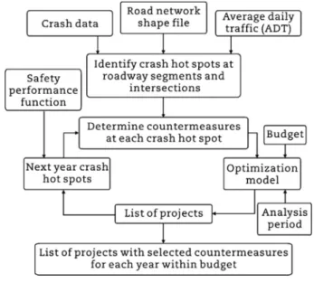
This section presents the formulation of TSMS model used in this research. The primary parameter of this model, crash hot spots identification, is discussed briefly. Identifying crash hot spots requires crash data analysis which is followed by field investigation to identify appropriate treatment types. The al-gorithm for identifying the best combination of safety projects is illustrated inFig. 1. This process consists of two main steps which are identification of crash hot spots and potential countermeasures and allocation of funding. Each step is discussed in detail in the following subsections.
3.1. Identification of crash hot spots
Traffic crashes are rare and random events having a tendency to cluster together at certain locations. The straightforward process of plotting crash map reveals clustering characteris-tics of crash occurrence. Road conditions, weather condition, horizontal alignment of roadway, grade and lighting condi-tions are the most contributing factors of crashes. In this
research, crash frequency was calculated for each segment using five years of crash data (2010e2014). As the length of each segment is different, the crash frequency was normal-ized by one mile, so that the segments can be compared. In order to identify crash hot spots, the EB method has been implemented. In this method, the expected crashes were calculated using the SPF of two-lane two-way roadways from HSM.
Sometimes, decision makers or engineers might have different objectives to improve the safety of the network, such as reducing overall crash frequency and reducing severe crashes. This research considered both of the objectives to identify the best combination of safety improvement projects. In the process of identifying the projects, priority was given to the hot spots that were involved with fatal-and-injury crashes.
3.2. Funding allocation strategy
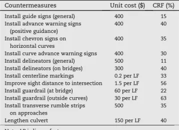
After identifying crash hot spots, the next step is to conduct field evaluation to identify safety countermeasures. A list of the possible low-cost safety countermeasures associated with unit cost for county paved roads are summarized inTable 1. The WYT2/LTAP uses these low-cost safety countermeasures to enhance the safety of county paved roads. When a major safety improvement is needed, it is normally combined with other major pavement rehabilitation projects. At each location, the best countermeasure is chosen based on CRF and cost with consideration of the overall safety budget. It's an optimization method where the objective function is to minimize the predicted crash frequency within budget by selecting the best combination of safety improvement projects on roadways with higher ADT.
3.3. The optimization model
The proposed TSMS for county paved roads considers CRF as well as local conditions of crash frequency and ADT. The
objective of the developed model is to minimize the overall predicted crashes on the segments with high traffic volume giving the priority to the segments experiencing fatal-and-injury crashes. The model is described as Eq.(1).
8 > > < > > : Minimize Pn i¼1 Ni Minimize Pn i¼1 Nf&Ii (1)
where Ni and Nf&Ii represent the predicted crashes and fatal-and-injury crashes on road i, respectively. This is a combinatorial optimization problem where one must select a collection of projects of minimum value while satisfying some constraint. The predicted crashesNiis the crashes of the segment multiplied by the CRF if the segment is selected for improvements. This model is a multi-level optimization where two objective functions were consid-ered as shown in Eq.(2). More formally, the problem can be written as 8 > > > > > > > > < > > > > > > > > : Minimize Pn i¼1 Ni Minimize Pn i¼1 Nf&Ii Subject to Pn i¼1
safety improvement costixi
!
Budget
xi2f0; 1g
(2) wherexiis an integer equal to 1 if the project is selected and 0 if it is not selected. The best combination of safety improvement projects are selected using linear programming methods.
4.
Case study for data collection (county
paved roads in Wyoming)
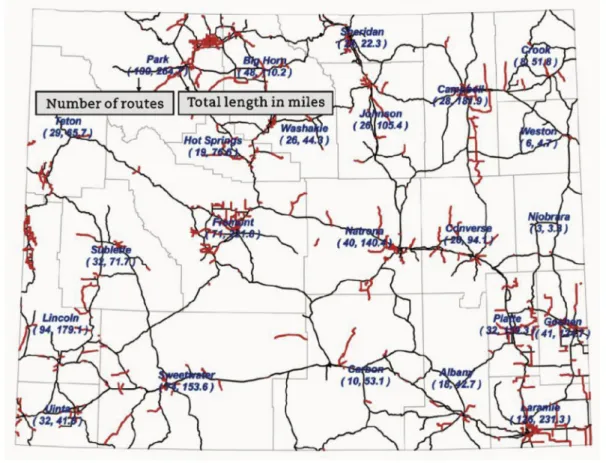
Table 2summarizes data sources with the type and number of collected data units for the case study.Fig. 2shows the study area representing the county paved roads totaling 2444 miles divided into 917 routes. The datasets obtained from WYDOT and WYT2/LTAP are described briefly in the following subsections.
4.1. County paved roads
The road inventory of county paved roads used in this research were obtained from WYDOT containing information on road identification number (RIN), primary name of the road, beginning and ending milepost. There are 917 county paved roads in Wyoming with 2444 miles.
4.2. Crash data
The crash data for the study area was obtained from WYDOT and the base bulk data was used for this research. The base bulk dataset contains information on accident time, location, accident type, impact type, severity level, reported weather conditions, lighting condition, road condition, and roadway geometry for each accident. For this study, crash severity, accident route, location, relation to intersection, and crash date are needed. Crash data from January 2010 to December 2014 were used to ensure there were no major changes of roadway geometrics in the study area.
4.3. Functional classification
Functional classification of county paved roads was also ob-tained from WYDOT. All roads were divided into rural and urban land-use. In each land-use, the roads are classified into arterial, collector and locals. Some arterial and collectors are subdivided into major and minor.
4.4. Traffic counts
A total of 144 traffic counts were conducted to prioritize the functional classification of roadways used in the optimization model.
4.5. Data base for TSMS
All variables used in this study were collected from different sources for each roadway segment and then combined in a comprehensive data base for the optimization model. The Table 1eCRFs and costs of safety countermeasures for
paved county roads.
Countermeasures Unit cost ($) CRF (%)
Install guide signs (general) 400 15
Install advance warning signs (positive guidance)
400 40
Install chevron signs on horizontal curves
400 35
Install curve advance warning signs 400 30
Install delineators (general) 500 11
Install delineators (on bridges) 300 40
Install centerline markings 0.2 per LF 33
Improve sight distance to intersection 1.5 per LF 56
Install guardrail (at bridge) 60 per LF 22
Install guardrail (outside curves) 30 per LF 63
Install transverse rumble strips on approaches
500 35
Lengthen culvert 150 per LF 40
Note: LF is linear feet.
Table 2eFeatures and data collected for county roads.
Feature Data source Quantity Units Data types
County paved roads WYDOT 917 Roads GIS layer of county paved roads
Crash data WYDOT 5 years Events Crash locations
Functional classification WYT2/LTAP 2250 Segments Arterial, collector and rural
combined dataset contained beginning and ending mile-posts, crash frequency, functional class, selected counter-measure with associated CRF, and cost for each roadway segment. Functional classification of roadways was incor-porated to give a higher priority to the segments with higher traffic volumes. A sample dataset for the model is shown in Table 3.
5.
Preliminary analysis
A preliminary analysis was conducted on the crash data to examine crash severity in the network. It is important to mention that not only intersection-related crashes were considered. In Table 4 the intersection-related and
not-Fig. 2eLocations of county paved roads.
Table 3eCombined dataset for implementing TSMS model.
Route Beg. milepost End milepost Crash freq. Crash freq. per mile Functional class Countermeasure CRF Cost ($)
ML5349B 7.740 7.870 5 38 16 3 0.35 55,200 ML8448B 0.000 0.080 3 38 16 5 0.11 11,200 ML7650B 1.960 2.464 6 12 16 2 0.40 25,600 ML5349B 2.860 3.640 9 12 16 4 0.30 9600 ML7650B 3.464 3.920 3 7 16 6 0.40 4800 ML5338B 4.175 4.790 4 7 16 1 0.15 9600 ML5716B 7.514 8.514 6 6 16 6 0.40 4800
Table 4eCrashes on county roads from 2010 to 2014.
Crash type Not-intersection-related Intersection-related Total
Frequency Percentage (%) Frequency Percentage (%)
Fatal crashes 11 34.8 3 15.1 14
Injury crashes 285 67 352
Property damage only 506 59.5 382 82.5 888
Unknown 49 5.8 11 2.4 60
intersection-related crashes are divided into three crash severity, fatal, injury, and property damage only. It can be seen that 34.8% of not-intersection-related crashes were fatal and injury.
In order to identify the best combination of safety improvement projects, it is important to determine the traffic
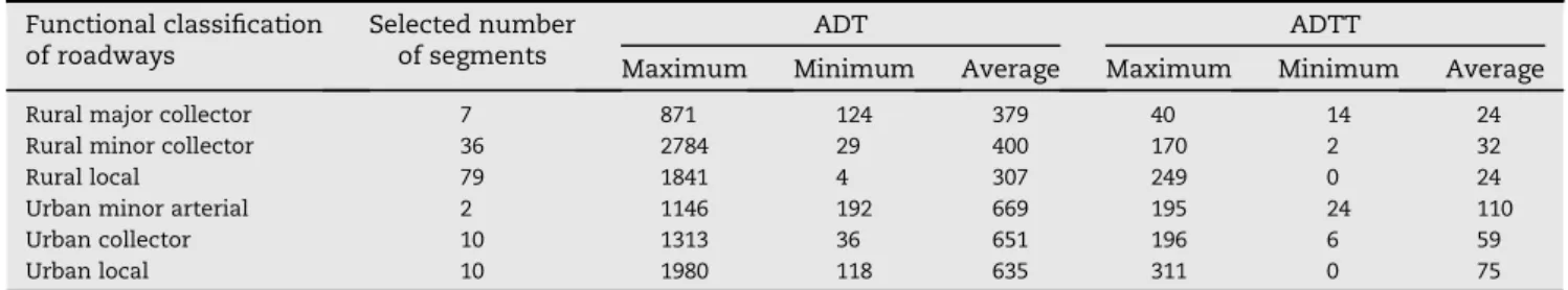
counts for each segment. There is a total of 917 county roads in Wyoming. Traffic counts are not available for all roads but the functional classes of these roadways are available. A sample data collection was conducted to determine average traffic counts of each functional class. A total of 144 traffic counts were conducted in the summer of 2014. Table 5
Table 5eADT&average daily truck traffic (ADTT) by functional classification on selected segments. Functional classification
of roadways
Selected number of segments
ADT ADTT
Maximum Minimum Average Maximum Minimum Average
Rural major collector 7 871 124 379 40 14 24
Rural minor collector 36 2784 29 400 170 2 32
Rural local 79 1841 4 307 249 0 24
Urban minor arterial 2 1146 192 669 195 24 110
Urban collector 10 1313 36 651 196 6 59
Urban local 10 1980 118 635 311 0 75
Table 6eSelected crash hot spots using EB method.
Route Beg. milepost End milepost Crash freq. Fatal and injury ADT Expected crashes (p) Index of effectiveness (q)
ML5314B 1.000 2.000 4 0 307 1.05 3.05 ML8658B 6.190 7.190 4 0 307 1.27 2.61 ML5849B 0.940 0.980 4 0 307 1.38 2.45 ML7860B 0.000 1.000 4 0 307 0.99 2.31 ML5349B 0.000 1.000 4 0 669 1.49 2.29 ML5836B 1.790 2.790 4 3 379 1.49 2.29 ML7852B 14.950 15.950 4 0 400 1.49 2.29 ML8325B 0.090 0.180 3 1 400 1.12 2.18 ML7650B 0.960 1.960 5 0 669 2.04 2.12 ML7452B 1.000 1.520 3 1 400 1.23 2.01 ML7453B 0.000 1.000 3 1 307 1.23 2.01 ML7454B 1.000 2.000 3 2 307 1.23 2.01 ML7676B 0.000 1.000 3 0 400 1.23 2.01 ML5531B 2.073 3.073 3 0 651 1.24 2.01 ML5349B 5.842 6.842 4 0 669 1.73 1.96 ML6257B 2.150 3.150 3 0 400 1.22 1.95 ML7461B 3.610 4.360 4 0 307 1.80 1.89 ML7673B 3.660 4.660 4 0 400 1.80 1.89 ML5584B 4.112 5.112 6 1 651 2.88 1.82 ML5349B 5.095 5.842 9 0 669 4.15 1.75 ML5789B 2.490 3.500 3 0 307 1.42 1.75 ML8647B 3.000 4.000 3 0 400 1.43 1.73 ML7852B 13.950 14.950 6 0 400 3.15 1.68 ML8035B 2.300 3.270 3 0 379 1.49 1.67 ML5547B 2.790 3.790 3 0 400 1.49 1.67 ML5828B 5.000 5.714 3 0 307 1.49 1.67 ML7653B 0.000 1.000 3 1 307 1.49 1.67 ML7674B 8.070 9.070 3 0 400 1.49 1.67 ML8448B 3.376 4.376 3 0 669 1.49 1.67 ML5339B 2.881 3.684 6 0 651 3.30 1.61 ML5338B 4.175 4.790 4 2 669 2.08 1.59 ML8450B 1.003 1.500 6 0 635 3.35 1.59 ML7650B 3.464 3.920 4 0 669 2.20 1.52 ML5716B 9.514 10.514 6 0 669 2.92 1.49 ML5349B 4.390 5.095 3 0 669 1.72 1.40 ML7963B 5.510 6.020 4 1 651 2.49 1.37 ML8030B 1.010 1.530 4 1 307 2.49 1.37 ML5322B 3.000 4.000 3 0 379 1.82 1.34 ML5339B 7.880 8.600 3 0 651 1.83 1.32 ML5365B 24.030 25.030 3 1 379 2.03 1.22 ML7704B 0.067 1.067 3 0 307 2.03 1.22
summarizes the average traffic counts for the six different functional classes of roadways. It can be seen that there is a significant difference of average ADTs between urban and rural classes.
6.
Data analysis
The data analysis section summarizes the analysis in three sections, crash hot spots, optimization process, and sensi-tivity analysis. The crash hot spots section identifies the lo-cations where increasing number of crashes occurred compared to the expected crashes using the appropriate SPF from HSM. Then, the optimization process identifies the pro-jects among the selected crash hot spots within the approxi-mate budget currently allocated to improve safety on county paved roads. Finally, a sensitivity analysis was conducted to identify the critical budget that gives the most benefit to society.
6.1. Crash hot spots
The EB method has been implemented to identify the crash hot spots.Table 6shows the list of the crash hot spots where the most of the crashes occur. The expected crashes of this table were calculated using the SPF of two-lane two-way roadways obtained from HSM. In this table, the last column is the index of effectiveness, which represents the increase of actual crashes compared to the expected crashes, if its value is greater than 1. There are a total of 41 crash hot spots identified from all 3762 segments, because of their higher values for one mile in length.
6.2. Optimization
The limited funding is not adequate to fund all these crash hot spots identified in the previous sections. An optimization model was implemented to identify the best combination of safety improvement projects within the limited budget. The
Table 7eLow-cost safety countermeasures.
Countermeasure ID Countermeasures Crash reduction factors (%) Cost ($)
1 Install guide signs (general) 15 9600
2 Install advance warning signs (positive guidance) 40 25,600
3 Install chevron signs on horizontal curves 35 55,200
4 Install curve advance warning signs 30 9600
5 Install delineators (general) 11 11,200
6 Install delineators (on bridges) 40 4800
Table 8eSelected safety improvement projects for $250,000 spending.
Route Beg. milepost End milepost Crash freq. Fatal and injury ADT Countermeasure CRF Cost ($)
ML8658B 6.190 7.190 4 0 307 5 0.11 11,200 ML7860B 0.000 1.000 4 0 307 4 0.30 9600 ML5349B 0.000 1.000 4 0 669 6 0.40 4800 ML5836B 1.790 2.790 4 3 379 1 0.15 9600 ML7852B 14.950 15.950 4 0 400 6 0.40 4800 ML8325B 0.090 0.180 3 1 400 5 0.11 11,200 ML7650B 0.960 1.960 5 0 669 6 0.40 4800 ML7452B 1.000 1.520 3 1 400 5 0.11 11,200 ML7453B 0.000 1.000 3 1 307 1 0.15 9600 ML7454B 1.000 2.000 3 2 307 5 0.11 11,200 ML5349B 5.842 6.842 4 0 669 5 0.11 11,200 ML7461B 3.610 4.360 4 0 307 5 0.11 11,200 ML5584B 4.112 5.112 6 1 651 2 0.40 25,600 ML5349B 5.095 5.842 9 0 669 4 0.30 9600 ML7852B 13.95 14.950 6 0 400 4 0.30 9600 ML7653B 0.000 1.000 3 1 307 4 0.30 9600 ML8448B 3.376 4.376 3 0 669 6 0.40 4800 ML5338B 4.175 4.790 4 2 669 6 0.40 4800 ML8450B 1.003 1.500 6 0 635 5 0.11 11,200 ML5716B 9.514 10.514 6 0 669 5 0.11 11,200 ML5349B 4.390 5.095 3 0 669 6 0.40 4800 ML7963B 5.510 6.020 4 1 651 6 0.40 4800 ML8030B 1.010 1.530 4 1 307 5 0.11 11,200 ML5322B 3.000 4.000 3 0 379 1 0.15 9600 ML5339B 7.880 8.600 3 0 651 5 0.11 11,200 ML5365B 24.030 25.030 3 1 379 1 0.15 9600 Total 108 15 248,000
optimization model developed in this research was based on the following principles.
Countermeasures with higher CRF and lower cost are the most cost effective.
Roadways with high traffic volume should have higher priority when selecting safety projects.
Table 7 shows the list of the low-cost safety countermeasures considered for county paved roads. In order to demonstrate the characteristics of the proposed TSMS, general safety countermeasures were selected. Future
implementation of the proposed TSMS would require conducting field visitation to each hot spot to identify potential safety improvements.
The optimization model proposed in this research was used to select the best combination of safety improvement projects. For each crash hot spot, expected crashes were determined by multiplying CRF and crashes occurred. The objective was to minimize the overall expected number of crashes by selecting the projects involved with fatal and injury after implementing the safety countermeasures within budget.
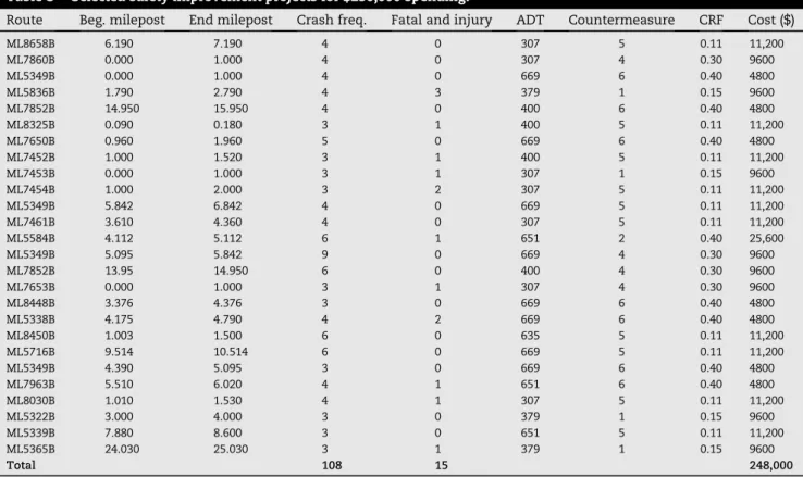
WYDOT currently allocates around $500,000 annually to improve the safety of all county roads in the state. Assuming that half of the funding will be spent on paved roads, the annual budget is set at $250,000. Running the optimization model resulted in the list of projects shown inTable 8. The implementation of the selected countermeasures is expected to reduce crashes by 82 (from 160 to 78).
6.3. Sensitivity analysis
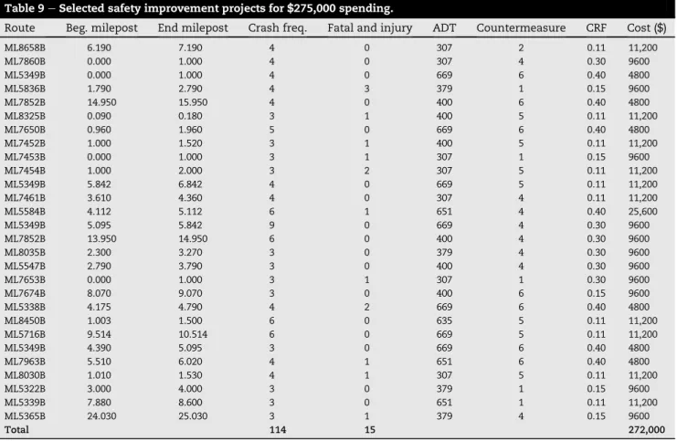
Decision makers need to allocate appropriate funding to pro-vide the maximum benefit to society. In this study, the appropriate budget was determined based on the expected crash reduction. The optimization model was performed at different budgets levels between $100,000 and $800,000.Fig. 3 shows the trend in expected crashes reduction as budget increases. It can be seen that the slope of the estimated crash reduction is higher when budget is between $100,000 and $275,000 than the one with budget between $275,000
Fig. 3eTSMS performances for different budgets.
Table 9eSelected safety improvement projects for $275,000 spending.
Route Beg. milepost End milepost Crash freq. Fatal and injury ADT Countermeasure CRF Cost ($)
ML8658B 6.190 7.190 4 0 307 2 0.11 11,200 ML7860B 0.000 1.000 4 0 307 4 0.30 9600 ML5349B 0.000 1.000 4 0 669 6 0.40 4800 ML5836B 1.790 2.790 4 3 379 1 0.15 9600 ML7852B 14.950 15.950 4 0 400 6 0.40 4800 ML8325B 0.090 0.180 3 1 400 5 0.11 11,200 ML7650B 0.960 1.960 5 0 669 6 0.40 4800 ML7452B 1.000 1.520 3 1 400 5 0.11 11,200 ML7453B 0.000 1.000 3 1 307 1 0.15 9600 ML7454B 1.000 2.000 3 2 307 5 0.11 11,200 ML5349B 5.842 6.842 4 0 669 5 0.11 11,200 ML7461B 3.610 4.360 4 0 307 4 0.11 11,200 ML5584B 4.112 5.112 6 1 651 4 0.40 25,600 ML5349B 5.095 5.842 9 0 669 4 0.30 9600 ML7852B 13.950 14.950 6 0 400 4 0.30 9600 ML8035B 2.300 3.270 3 0 379 4 0.30 9600 ML5547B 2.790 3.790 3 0 400 4 0.30 9600 ML7653B 0.000 1.000 3 1 307 1 0.30 9600 ML7674B 8.070 9.070 3 0 400 6 0.15 9600 ML5338B 4.175 4.790 4 2 669 6 0.40 4800 ML8450B 1.003 1.500 6 0 635 5 0.11 11,200 ML5716B 9.514 10.514 6 0 669 5 0.11 11,200 ML5349B 4.390 5.095 3 0 669 6 0.40 4800 ML7963B 5.510 6.020 4 1 651 6 0.40 4800 ML8030B 1.010 1.530 4 1 307 5 0.11 11,200 ML5322B 3.000 4.000 3 0 379 1 0.15 9600 ML5339B 7.880 8.600 3 0 651 1 0.11 11,200 ML5365B 24.030 25.030 3 1 379 4 0.15 9600 Total 114 15 272,000
and $800,000. Therefore, $275,000 is the appropriate budget level based on the assumptions of the optimization model. The selected safety improvement projects based on $275,000 funding level can be seen inTable 9.
7.
Conclusions
The state of Wyoming does not currently have a traffic safety management system (TSMS) to optimize the use of safety funds. In this study, an optimization methodology was devel-oped to identify the best combination of safety improvement projects that utilizes limited available resources. The devel-oped methodology was implemented on the county paved road network consisting of 917 roads with 2444 miles. This meth-odology minimized the overall expected crashes by selecting the best combination of safety improvement projects. A sensitivity analysis was also conducted to identify the most appropriate budget to provide maximum benefit to society.
The developed methodology can be highlighted as follows It is tailored specifically to county paved roads.
It considers countermeasures CRF, countermeasures cost, functional classification of roadways, and annual safety budget.
It provides a higher priority to projects on roadways with higher ADTs and functional classification.
It identifies the best set of safety improvement projects to minimize the overall expected crashes based on a specific budget level.
It requires field evaluation and crash analysis to identify crash hot spots and appropriate safety countermeasures. It identifies the minimum budget needed to achieve the
maximum benefits to society in terms of crashes reduction. This proposed methodology can be implemented on the Wyoming state highway system with minor modifications. Other states can follow the same process described in this paper to develop their own TSMS. When public agencies have limited budgets, it becomes more important to allocate re-sources in a cost effective manner. This study demonstrated how optimization techniques can be utilized to justify budget setting for safety improvements and then allocate the funding to achieve the maximum reduction in crashes.
Acknowledgments
The authors would like to thank the Wyoming LTAP Center for supporting this research study.
r e f e r e n c e s
AASHTO, 2010. The Highway Safety Manual, American Association of State Highway Transportation Professionals. AASHTO, Washington DC.
Abdel-Aty, M.A., Radwan, E.A., 2000. Modeling traffic accident occurrence and involvement. Accident Analysis&Prevention 32 (5), 633e642.
Ahmed, M., Huang, H., Abdel-Aty, M., et al., 2011. Exploring a Bayesian hierarchical approach for developing safety performance functions for a mountainous freeway. Accident Analysis&Prevention 43 (4), 1581e1589.
Anderson, T., 2009. Kernel density estimation and K-means clustering to profile road accident hotspots. Accident Analysis&Prevention 41 (3), 359e364.
Cafiso, S., Di Draziano, A., Di Silvestro, G., et al., 2010. Development of comprehensive accident models for two-lane rural highways using exposure, geometry, consistency and context variables. Accident Analysis&Prevention 42 (4), 1072e1079.
Cheng, W., Washington, S., 2008. New criteria for evaluating methods of identifying hot spots. Transportation Research Record 2083, 76e85.
Chin, H., Quddus, M.A., 2003. Applying the random effect negative binomial model to examine traffic accident occurrence at signalized intersections. Accident Analysis &Prevention 35 (2), 253e259.
Elvik, R., 2008. Comparative analysis of techniques for identifying locations of hazardous roads. Transportation Research Record 2083, 72e75.
ESRI, 2010. How Spatial Autocorrelation: Moran's I (Spatial Statistics) Works Available at:http://resources.esri.com/help/ 9.3/ArcGISengine/java/Gp_ToolRef/Spatial_Statistics_tools/ how_spatial_autocorrelation_colon_moran_s_i_spatial_ statistics_works.htm(Accessed 25 January 2012).
Getis, A., Ord, J.K., 1992. The analysis of spatial association by use of distance statistics. Geographical Analysis 24 (3), 189e206. Hauer, E., Allery, B.K., Kononov, J., et al., 2004. How best to rank
sites with promise. Transportation Research Record 1897, 48e54.
Jovanis, P., Chang, H., 1986. Modeling the relationship of accidents to miles traveled. Transportation Research Record 1068, 42e51.
Miaou, S.P., Lord, D., 2012. Modeling traffic crash-flow relationships for intersections. Transportation Research Record 1840, 31e40.
Mishra, S., Golias, M.M., Sharma, S., et al., 2015. Optimal funding allocation strategies for safety improvements on urban intersections. Transportation Research Part A: Policy and Practice 75, 113e133.
Montella, A., 2010. A comparative analysis of hotspot identification methods. Accident Analysis & Prevention 42 (2), 571e581.
Persuad, B., Lyon, C., Nguyen, T., 1999. Empirical Bayes procedure for ranking sites for safety investigation by potential for safety improvement. Transportation Research Record 1665, 7e12. Saha, P., 2014. Modeling Effectiveness of Variable Speed Limit
(VSL) Corridors on Crashes and Road Closures (PhD thesis). The University of Wyoming, Laramie.
Saha, P., Ahmed, M.M., Young, R.K., 2015. Safety effectiveness of variable speed limit system in adverse weather conditions on challenging roadway geometry. Transportation Research Record 2521, 45e53.
Saha, P., Ksaibati, K., 2015. A risk-based optimization methodology for managing county paved roads. International Journal of Pavement Engineering 17 (10), 913e923.
Tegge, R.A., Jo, J., Ouyang, Y., 2010. Development and Application of Safety Performance Functions for Illinois. Illinois Center for Transportation, Illinois.
WYDOT, 2008. WYDOT and General Fund Appropriations for Highways. WYDOT, Cheyenne.
WYDOT, 2015a. Statewide Conditions of County Paved Roads in Wyoming. WYDOT, Cheyenne.
WYDOT, 2015b. Wyoming's 2014 Report on Traffic Crashes. WYDOT, Cheyenne.
Khaled Ksaibati, Ph.D., P.E.obtained his BS degree from Wayne State University and his MS and Ph.D. degrees from Purdue Univer-sity. Dr. Ksaibati worked for the Indian Department of Transportation for a couple of years prior to coming to the University of Wyoming in 1990. He was promoted to an associate professor in 1997 and full professor in 2002. Dr. Ksaibati has been the director of the Wyoming Technology Transfer Center since 2003.
Promothes Saha, Ph.D.obtained his MS
de-gree in 2011 and Ph.D. dede-gree in 2014 from University of Wyoming with an emphasis in transportation engineering. After that he is working as a postdoctor in Wyoming Tech-nology Transfer Center, University of Wyoming. His current research interests include pavement management system and transportation safety.