PARAMETRIC CONTROL OF FAMILYWISE
ERROR RATES WITH DEPENDENT
P
-VALUES
by
Richard E. Blakesley
BS Psychology, Rochester Institute of Technology, 2001
Submitted to the Graduate Faculty of
the Department of Biostatistics
Graduate School of Public Health in partial fulfillment
of the requirements for the degree of
Doctor of Philosophy
University of Pittsburgh
UNIVERSITY OF PITTSBURGH
GRADUATE SCHOOL OF PUBLIC HEALTH
This dissertation was presented
by Richard E. Blakesley It was defended on July 28th 2008 and approved by Dissertation Director:
Sati Mazumdar, PhD, Professor, Department of Biostatistics Graduate School of Public Health, University of Pittsburgh
Gong Tang, PhD, Assistant Professor, Department of Biostatistics Graduate School of Public Health, University of Pittsburgh
Howard E. Rockette, PhD, Professor, Department of Biostatistics Graduate School of Public Health, University of Pittsburgh
Charles F. Reynolds III, MD, Professor, Department of Psychiatry School of Medicine, University of Pittsburgh
Eleanor Feingold, PhD, Associate Professor, Department of Human Genetics Graduate School of Public Health, University of Pittsburgh
Sanat K. Sarkar, PhD, Professor, Department of Statistics Fox School of Business and Management, Temple University
Copyright c by Richard E. Blakesley 2008
PARAMETRIC CONTROL OF FAMILYWISE ERROR RATES WITH DEPENDENT P-VALUES
Richard E. Blakesley, PhD
University of Pittsburgh, 2008
Many research areas require multiple outcomes. For example, neuropsychological hypotheses may not be testable using a single measure. Similarly, genetic researchers frequently exam-ine multiple markers across the genome. Examining multiple hypotheses requires the use of multiple testing procedures (MTPs) to control Type I error. The application of MTPs is significant to public health researchers because of the danger of declaring false inferences. Researchers need MTPs to control such error while maintaining power to detect real ef-fects. Two specific error rates include the familywise error rate (FWER) and the generalized FWER (k-FWER). We begin with an examination of ten FWER MTPs with respect to a key multiple testing issue, p-value dependence. This preliminary look illuminated the benefit of stepwise methods over single-step counterparts, the strengths and challenges of nonparametric, resampling-based methods, and the insufficiency of parametric methods in addressing p-value dependence. This dissertation continues with proposals for new, para-metric, step-down (SD) MTPs that incorporate correlation information with the aim to control the FWER and k-FWER. By simulation studies and applications to a microarray data example, we compared these proposed methods against several existing MTPs, includ-ing the nonparametric SD minP and SDk-minP methods, considered here as the benchmark MTPs. The proposed FWER and k-FWER methods approximated the error and power of the comparison SD minP and SD k-minP methods more closely than the other parametric MTPs. The proposed FWER method demonstrated notable FWER control. The proposed
k-FWER method exhibited a degree of error, suggesting the need for further refinement.
TABLE OF CONTENTS
PREFACE . . . xi
1.0 INTRODUCTION . . . 1
1.1 The Multiple Hypothesis Testing Problem . . . 1
1.2 Overview and Aims . . . 2
1.2.1 Aim 1: Comparisons of Methods for Multiple Hypothesis Testing in Neuropsychological Research . . . 3
1.2.2 Aim 2: Considering P-Value Dependence in a Stepwise Multiple Test-ing Procedure . . . 4
1.2.3 Aim 3: Controlling the Generalized Familywise Error Rate with P -Value Dependence . . . 5
2.0 COMPARISONS OF METHODS FOR MULTIPLE HYPOTHESIS TESTING IN NEUROPSYCHOLOGICAL RESEARCH . . . 6
2.1 Abstract. . . 7
2.2 Introduction . . . 8
2.3 P-Value Adjustment Methods . . . 9
2.3.1 Bonferroni-Class Methods . . . 10 2.3.2 Sidak-Class Methods . . . 11 2.3.3 Resampling-Class Methods . . . 12 2.3.4 Illustrative Example . . . 13 2.4 Sensitivity Analysis . . . 15 2.4.1 Data . . . 15 2.4.2 Analysis . . . 16 v
2.4.3 Results . . . 16
2.5 Simulation Study . . . 19
2.5.1 Methods . . . 19
2.5.2 Results . . . 22
2.5.2.1 Compound-Symmetry - Uniform Hypothesis Set . . . 23
2.5.2.2 Compound-Symmetry - Split Hypothesis Set . . . 25
2.6 Discussion . . . 27
2.7 Acknowledgements . . . 29
3.0 CONSIDERING P-VALUE DEPENDENCE IN A STEPWISE MUL-TIPLE TESTING PROCEDURE . . . 30
3.1 Abstract. . . 31
3.2 Introduction . . . 32
3.3 Multiple Testing Procedures . . . 33
3.3.1 Notation . . . 33
3.3.2 Parametric FWER Control with IndependentP-Values . . . 33
3.3.3 Nonparametric FWER Control with Dependent P-Values . . . 36
3.3.4 Parametric FWER Control with Dependent P-Values . . . 37
3.3.4.1 Areas for Improvement . . . 37
3.3.5 Proposed Method . . . 38
3.4 Simulation Methods . . . 39
3.4.1 Data Generation . . . 39
3.4.2 Adjusted P-Value Calculation . . . 42
3.4.3 Performance Assessment . . . 43
3.5 Simulation Results . . . 43
3.5.1 Compound Symmetry Series . . . 43
3.5.2 Block symmetry and Decreasing Dependence Series . . . 44
3.6 Example. . . 47
3.7 Discussion . . . 49
3.8 Acknowledgements . . . 50
4.0 CONTROLLING THE GENERALIZED FAMILYWISE ERROR RATE
WITH P-VALUE DEPENDENCE . . . 51
4.1 Abstract. . . 52
4.2 Introduction . . . 53
4.3 k-FWER Multiple Testing Procedures . . . 54
4.3.1 Notation . . . 54 4.3.2 Parametric k-FWER MTPs. . . 55 4.3.3 Nonparametric k-FWER MTPs . . . 57 4.3.4 Proposed Method . . . 58 4.4 Simulation Methods . . . 61 4.5 Simulation Results . . . 63
4.5.1 Uniform Hypothesis Set . . . 63
4.5.2 Split Hypothesis Set . . . 68
4.6 Example. . . 68
4.7 Discussion . . . 71
4.8 Acknowledgements . . . 72
5.0 CONCLUSION AND DISCUSSION . . . 73
APPENDIX A. SUPPLEMENTARY MATERIALS: COMPARISONS OF METHODS FOR MULTIPLE HYPOTHESIS TESTING IN NEUROPSY-CHOLOGICAL RESEARCH . . . 74
APPENDIX B. SUPPLEMENTARY MATERIALS: CONSIDERING P -VALUE DEPENDENCE IN A STEPWISE MULTIPLE TESTING PROCEDURE . . . 81
BIBLIOGRAPHY . . . 84
LIST OF TABLES
1.1 Hypothesis Truth vs. Hypothesis Decisions . . . 1
2.1 Illustrative Example: ObservedP-Values and AdjustedP-Values by Class and Method . . . 14
2.2 Neuropsychological Outcome Correlation Matrix . . . 17
2.3 CS Simulation Series Parameters . . . 20
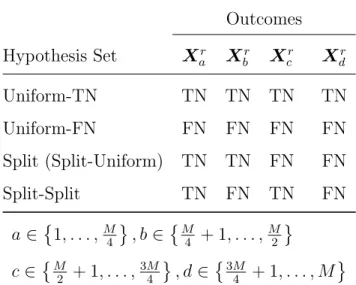
3.1 Hypothesis Sets . . . 42
3.2 Example Summary of Sensitivity and Rejected Hypothesis Count . . . 47
4.1 Example Summary of Sensitivity and Rejected Hypothesis Count . . . 70
A1 Adjusted P-Values by Method across Neuropsychological Outcomes . . . 76
A2 BS Simulation Series Parameters . . . 77
LIST OF FIGURES
2.1 Adjusted P-Values by Method across Neuropsychological Outcomes . . . 18
2.2 P-Value Adjustment Method Performance across Compound-Symmetry Cor-relation Structures
Type I Error and Power Estimates for Uniform Hypothesis Set . . . 24
2.3 P-Value Adjustment Method Performance across Compound-Symmetry Cor-relation Structures
Type I Error and Power Estimates for Split Hypothesis Set . . . 26
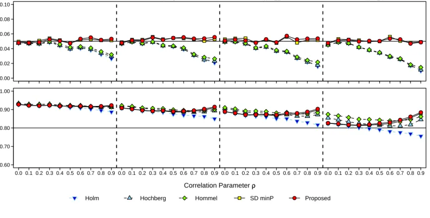
3.1 Multiple Testing Procedure Performance for the Compound Symmetry Series FWER and Average Power Estimates for Uniform Hypothesis Set. . . 45
3.2 Multiple Testing Procedure Performance for the Compound Symmetry Series FWER and Average Power Estimates for Split Hypothesis Set . . . 46
3.3 Example MTP Adjusted P-Values against SD minP P-Values . . . 48
4.1 Multiple Testing Procedure k-FWER and Average Performance for the Uni-form Hypothesis Set, Low k= M4 . . . 64
4.2 Multiple Testing Procedure k-FWER and Power Performance for the Uniform Hypothesis Set, Moderatek = M2 . . . 65
4.3 Multiple Testing Procedure k-FWER and Power Performance for the Uniform Hypothesis Set, High k= 3M4 . . . 66
4.4 Multiple Testing Procedure k-FWER and Power Performance for the Split Hypothesis Set . . . 67
4.5 Example MTP Adjusted P-Values against Step-Down k-minP P-Values . . . 69
A1 Bootstrap Empirical MinP Null Distributions for the Illustrative Example . . 75
A2 P-Value Adjustment Method Performance across Block-Symmetry Correlation Structures
Type I Error and Power Estimates for Uniform Hypothesis Set . . . 78
A3 P-Value Adjustment Method Performance across Block-Symmetry Correlation Structures
Type I Error and Power Estimates for Split - Uniform Hypothesis Set . . . . 79
A4 P-Value Adjustment Method Performance across Block-Symmetry Correlation Structures
Type I Error and Power Estimates for Split - Split Hypothesis Set . . . 80
B1 Multiple Testing Procedure Performance for the Block Symmetry and Decreas-ing Dependence Series
FWER and Average Power Estimates for the Uniform Hypothesis Set . . . . 82
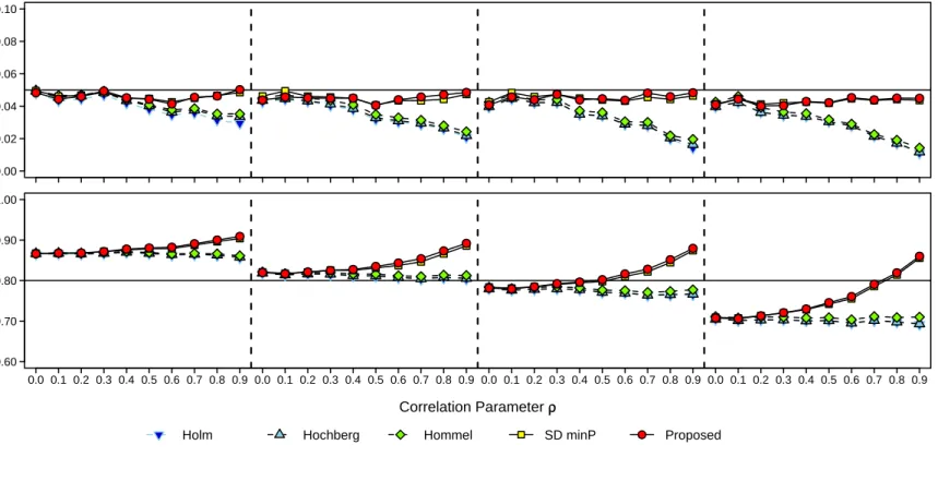
B2 Multiple Testing Procedure Performance for the Block Symmetry Series FWER and Average Power Estimates for the Split-Uniform and Split-Split Hypothesis Sets . . . 83
PREFACE
I am grateful for all the learning opportunities provided to me, including delving into re-search, engaging in real data analyses, contending with homework, or observing the task approaches of others. The supervisors, members of my committee, course faculty, collabo-rators, and students with whom I have interacted have all had small parts in shaping my way of the statistician. Through the challenging process, my friends and family have kept me focused through their love and support. For all of this, I am thankful.
This research was supported by the National Institute of Mental Health (NIMH) T32 MH073451, the NIMH P30 MH071944, the NIMH R01 MH072947, and the National Institute on Aging P01 AG020677.
1.0 INTRODUCTION
1.1 THE MULTIPLE HYPOTHESIS TESTING PROBLEM
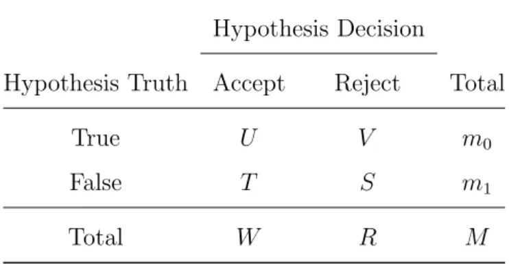
As scientific research advances, so does the complexity of data analysis. Increasingly, re-searchers collect data with multiple, correlated outcomes measures and/or multiple compar-ison groups, from which arises the problem of multiplicity (Pocock,1997). Such informative studies increase the risk of making a Type I error, defined as an erroneous, hypothesis test decision to reject a null hypothesis. As we do not know the actual truth of the hypotheses, we use hypothesis testing to make decisions to reject or accept (not reject) a null hypothesis. Table 1.1 summarizes the possibilities of hypothesis truths and decisions.
Table 1.1: Hypothesis Truth vs. Hypothesis Decisions
Hypothesis Decision
Hypothesis Truth Accept Reject Total
True U V m0
False T S m1
Total W R M
This table denotes the counts of outcomes types with regard to the (unknown) hypothesis truth and the decision reached after hypothesis testing.
Researchers are concerned primarily with count of Type I errors, denoted by V. Many multiple testing procedures (MTPs) exist which attempt to control one of several functions
of V, including the familywise error rate (FWER), the generalized familywise error rate (k-FWER), the false discovery proportion (FDP), and the false discovery rate (FDR). We define these probabilities, or error rates, as follows:
FWER =P [V ≥1] (1.1) k-FWER =P [V ≥k] (1.2) FDP = V /R R >0 0 R= 0 (1.3) FDR =E[FDP] (1.4)
Many MTPs exist to control these error rates, often assuming independent p-values, or uncorrelated outcomes. Real data are rarely uncorrelated, such as our motivating data exam-ple, a study of neuropsychological performance among 100 depressed and 40 non-depressed elderly subjects (Butters et al., 2004). This study examined 17 correlated, neuropsycho-logical tests obtained from the 140 subjects using Bonferroni-adjusted t-test p-values. The Bonferroni method, a simple, conservative MTP, controls the FWER at the cost of reduced power. Furthermore, it is known to become more conservative with increasedp-value depen-dence. While other MTPs exist, their use in the literature is rare. These concerns prompted our initial research to understand the performance of the existing MTPs with regard to the correlation seen in real data. From this research, new ideas spurred the development of new parametric MTPs, designed to control the FWER and the k-FWER with dependent
p-values, or correlated outcomes, without sacrificing power. This dissertation documents the research and examination, through simulation studies and biometric examples, of both the proposed and existing MTPs.
1.2 OVERVIEW AND AIMS
The primary objective of this dissertation was to examine the properties of the existing and proposed FWER andk-FWER MTPs in the presence of correlated outcomes. Three specific aims are described briefly as follows:
Aim 1: Compare existing FWER MTPs with a sensitivity analysis (using neuropsycholog-ical data) and a simulation study.
Aim 2: Develop a stepwise, FWER MTP designed to account for p-value dependence, and compare the proposed and a selection of existing FWER MTPs using a microarray data example and a simulation study.
Aim 3: Extend the proposed FWER MTP, developed in Aim 2, to the k-FWER setting and compare the proposed and existingk-FWER MTPs using a microarray example and a simulation study.
We examined the MTP properties primarily by simulation in the context of two-sample, multivariate normal data and hypothesis testing by two-sample, equal-variance t-tests. We did not examine the MTP robustness in this dissertation, leaving this for future research. This includes robustness with regard to nonnormality, unequal variances, alternate test statistics, and/or multigroup comparisons.
This dissertation is organized into three self-contained manuscripts. Each manuscript addresses one specific aim, and is presented in Chapters 2,3, and4, respectively. Chapter5
offers some concluding thoughts and future directions.
1.2.1 Aim 1: Comparisons of Methods for Multiple Hypothesis Testing in Neu-ropsychological Research
There exist several MTPs designed to control the FWER, grouped into three classes. The Bonferroni-class methods comprise the Bonferroni,Holm(1979),Hochberg(1988), and Hom-mel (1988) methods. These parametric MTPs derive from the Bonferroni method or the global test ofSimes(1986), which also stems from the Bonferroni method. The three deriva-tives of the Bonferroni method incorporate stepwise features to improve power. The Sidak-class methods comprise the Sidak, Tukey-Ciminera-Heyse (TCH), Dubey/Armitage-Parmar (D/AP), and R2 Adjustment (RSA) methods (Sankoh et al., 1997). The parametric Sidak
method assumes uniform, independentp-values. The three derivatives, while sharing similar basic forms, deviate in the magnitude of multiplicity adjustment. Particularly, the D/AP and RSA methods incorporate measures of correlation under the notion of adjusting less
when the outcomes (and p-values) are correlated more strongly. The resampling-class meth-ods include the minP and step-down (SD) minP methmeth-ods (Westfall and Young,1993). These nonparametric MTPs use a bootstrap procedure to approximate the minimum p-value dis-tribution, from which adjusted p-values are calculated.
In neuropsychological research, multiple hypothesis testing with correlated outcomes is common, but frequently, the conservative Bonferroni method is the only MTP used by researchers. In this chapter, we sought to enhance understanding of the breadth of methods available with detailed explanations, an illustrative example, and a sensitivity analysis that elucidates the relative performance of the methods. We conducted a simulation study to examine the true FWER and power rates of the MTPs under a variety of conditions. We processed our findings into a set of guidelines for the use of these MTPs.
Manuscript/Presentation Status: A portion of this research was presented at the Western Psychiatric Institute and Clinic 6th Annual Research Day (Blakesley-Ball et al., 2006). The manuscript entitled ”Comparisons of Methods for Multiple Hypothesis Testing in Neuropsychological Research” is in press in Neuropsychology. Chapter 2 replicates this manuscript, with appropriate formatting modifications for the dissertation.
1.2.2 Aim 2: Considering P-Value Dependence in a Stepwise Multiple Testing Procedure
While nonparametric MTPs control the FWER while incorporating correlation information (Westfall and Young, 1993), the parametric D/AP and RSA methods, which attempt to incorporate correlation information, have not demonstrated the desired FWER control in simulation studies (Sankoh et al., 1997;Blakesley et al.,in press). We propose a parametric approximation that addresses several perceived issues with existing methods. We examined the properties of selected MTPs in a simulation study, and demonstrated their use with a biometric example.
Manuscript/Presentation Status: Earlier versions of this research have been pre-sented locally (Blakesley et al.,2008a), and at major statistical conferences (Blakesley et al.,
2007, 2008b). The manuscript in progress is presented in Chapter 3.
1.2.3 Aim 3: Controlling the Generalized Familywise Error Rate with P-Value Dependence
Several FWER MTPs have been extended to the k-FWER setting (Lehmann and Romano,
2005; Sarkar, 2005; Guo and Romano, 2007; Korn and Freidlin, 2008). The existing para-metric MTPs that incorporate correlation information had not been generalized, likely due to their unstable FWER control as demonstrated in previous simulations (Sankoh et al.,
1997; Blakesley et al., in press). By employing a theorem regarding the probability of u or more event occurrences (Feller, 1968), we adapt the parametric FWER in Aim 2, to the
k-FWER setting. Similarly, we examined the estimatedk-FWER and power of the proposed and existing k-FWER MTPs in both a simulation study and biometric example.
Manuscript/Presentation Status: This research has not yet been presented. Chapter
4 comprises the manuscript in progress.
2.0 COMPARISONS OF METHODS FOR MULTIPLE HYPOTHESIS TESTING IN NEUROPSYCHOLOGICAL RESEARCH
Richard E. Blakesley, BS 1, Sati Mazumdar, PhD1,2, Mary Amanda Dew, PhD 2,3, Patricia
R. Houck, MSH 2, Gong Tang, PhD 1, Charles F. Reynolds III, MD 2, Meryl A. Butters, PhD 2
1 Department of Biostatistics, University of Pittsburgh
2 Department of Psychiatry, University of Pittsburgh School of Medicine 3 Departments of Epidemiology and Psychology, University of Pittsburgh
Manuscript in Press: Neuropsychology This chapter retains the content and notation of the in press manuscript, but modifies some formatting, e.g., section and figure labeling, per ETD guidelines. Note that some notation introduced in this chapter differs from Chapters
3 and 4.
2.1 ABSTRACT
Hypothesis testing with multiple outcomes requires adjustments to control Type I error in-flation, which reduces power to detect significant differences. Maintaining the pre-chosen Type I error level is challenging when outcomes are correlated. This problem concerns many research areas, including neuropsychological research where multiple, interrelated assessment measures are common. Standard p-value adjustment methods include Bonferroni-, Sidak-, and resampling-class methods. In this report, the authors aimed to develop a multiple hy-pothesis testing strategy to maximize power while controlling Type I error. The authors conducted a sensitivity analysis, using a neuropsychological dataset, to offer a relative com-parison of the methods, and a simulation study to compare the robustness of the methods with respect to varying patterns and magnitudes of correlation between outcomes. The re-sults lead us to recommend the Hochberg and Hommel methods (step-up modifications of the Bonferroni method) for mildly correlated outcomes, and the step-down minP method (a resampling-based method) for highly correlated outcomes. The authors note caveats regard-ing the implementation of these methods usregard-ing available software.
Key words: Multiple hypothesis testing, correlated outcomes, familywise error rate, p -value adjustment, neuropsychological test performance data
2.2 INTRODUCTION
Neuropsychological datasets are typically comprised of multiple, partially-overlapping mea-sures, henceforth termed outcomes. A given neuropsychological domain, e.g., executive function, is composed of multiple interrelated sub-functions, and frequently, all sub-function outcomes of interest are subject to hypothesis testing. At a given α (critical threshold), the risk of incorrectly rejecting a null hypothesis, a Type I error, increases as more hypotheses are tested. This applies to all types of hypotheses, including a set of two-group compar-isons across multiple outcomes (e.g. differences between two groups across several cognitive measures), or multiple group comparisons within an analysis of variance framework (e.g. cognitive performance differences between several treatment groups and a control group). Collectively, we define these issues as the multiplicity problem (Pocock,1997).
Controlling Type I error at a desired level is a statistical challenge, further complicated by the correlated outcomes prevalent in neuropsychological data. By making adjustments to control Type I error, we increase the risk of incorrectly accepting a null hypothesis, a Type II error. In other words, we reduce power. Failure to control Type I error when examining multiple outcomes may yield false inferences, which may slow or sidetrack research progress. Researchers need strategies that maximize power while ensuring an acceptable Type I error rate.
Many methods exist to manage the multiplicity problem. Several methods are based on the Bonferroni and Sidak inequalities (Sidak, 1967; Simes, 1986). These methods ad-justα-values orp-values using simple functions of the number of tested hypotheses (Sankoh et al., 1997;Westfall and Young,1993). Holm (1979),Hochberg(1988), and Hommel(1988) developed Bonferroni derivatives incorporating stepwise components. Using rank-ordered
p-values, stepwise methods alter the magnitude of change as a function of p-value order. Mathematical proofs order these methods, from least to most power, as Bonferroni, Holm, Hochberg, and Hommel (Hochberg, 1988; Holm, 1979; Sankoh et al., 1997). The Tukey-Ciminera-Heyse (TCH), Dubey/Armitage-Parmar (D/AP) and R2 adjustment (RSA) meth-ods are single-step Sidak derivatives (Sankoh et al., 1997). Another class of methods uses resampling methodology. The bootstrap (single-step) minP and step-down minP methods
adjust p-values using the nonparametrically-estimated null distribution of the minimum p -value (Westfall and Young, 1993).
The Bonferroni-class methods and the Sidak method are theoretically valid with indepen-dent, uncorrelated outcomes only (Hochberg,1988;Holm,1979;Hommel,1988;Westfall and Young, 1993). The D/AP and RSA methods incorporate measures of correlation (Sankoh et al., 1997), and the resampling-class methods incorporate correlational characteristics via bootstrapping procedures (Westfall and Young,1993). However, it is unclear which methods perform better when analyzing correlated outcomes. Theoretical and empirical comparisons of these p-value adjustment methods have been limited in the breadth of methods compared and correlation structures explored (Hochberg and Benjamini, 1990; Hommel, 1988, 1989;
Sankoh et al., 1997, 2003; Simes, 1986). We aimed to identify the optimal method(s) for multiple hypothesis testing in neuropsychological research.
We organized this manuscript into several sections. First, we provide definitions and illustrations of ten p-value adjustment methods. Next, we describe a sensitivity analysis, defined as using statistical techniques in parallel to compare estimates, hypothesis inferences, and relative plausibility of the inferences (Saltelli et al., 2000; Verbeke and Molenberghs,
2001). Using a neuropsychological dataset, we compare the p-value adjustment methods by the adjusted p-value and inferences patterns. Following the sensitivity analysis, we detail a simulation study, which, by definition, permits the examination of measures of interest under controlled conditions. We examined the Type I error and power rates of the p-value adjustment methods under a systematic series of correlation and null hypothesis conditions. This allows us to compare the methods’ performance relative to simulation conditions, i.e., when the truth is known. Lastly, we offer guidelines for using these methods when analyzing multiple correlated outcomes.
2.3 P-VALUE ADJUSTMENT METHODS
Multiple testing adjustment methods may be formulated as either p-value adjustment (with higher adjusted p-values) or α-value adjustment (with lower adjusted α-values). We focus
on p-value adjustment method formulae as adjusted p-values allow direct interpretation against a chosen α-value, and eliminate the need for lookup tables or knowledge of complex hypothesis rejection rules (Westfall and Young,1993; Wright,1992). Furthermore, adjusted α-values are not supported by statistical software.
We describe the methods assuming a neuropsychological dataset with N subjects, be-longing to one of two groups, with M outcomes observed for each subject. The objective is to determine which outcomes are different between groups using two-sample t-tests. For the jth outcome, where j = {1,2, . . . , M}, there exists a null hypothesis, and an observed
p-valueresulting from testing the null hypothesis, denotedV(j),H0j, andpj, respectively.
The observedp-values are arranged such thatp1 ≥. . .≥pj ≥. . .≥pM. For each outcome,
we test the null hypothesis of no difference between the groups, i.e., the groups come from the same population. For any method, we calculate a sequence of adjusted p-values where we denotepaj as the adjustedp-value corresponding to pj.
2.3.1 Bonferroni-Class Methods
The parametric Bonferroni-class methods comprise the Bonferroni method and its deriva-tives. The Bonferroni method, defined as paj = min{M pj,1}, increases each p-value by
a factor of M to a maximum value of 1. Holm (1979) and Hochberg (1988) enhanced this single-step approach with stepwise adjustments which adjustp-values sequentially and main-tain the observedp-value order. Holm’s step-down approach begins by adjusting the smallest
p-value pM as paM = min{M pM,1}. For each subsequent pj, j = {M −1, M−2, . . . ,1},
paj is defined asmin{jpj,1}ifmin{jpj,1}is greater than or equal to all previously adjusted
p-values, paM through pa(j+1). Otherwise, it is the maximum of these previously adjustedp
-values. Therefore, we define Holmp-values aspaj =min{1, max[jpj,(j+ 1)pj+1, . . . , M pM]},
all of which are between 0 and 1. Hochberg’s method uses a step-up approach, such that paj = min{1p1,2p2, . . . , jpj}. Converse to Holm’s method, adjustment begins with the
largestp-value,pa1 = 1p1, and steps up to more significant p-values, where each subsequent
paj is the minimum ofjpj and the previously adjusted p-values, pa1 throughpa(j−1).
Hommel’s (1988) method is a derivative of Simes’ (1986) global test, which is derived from the Bonferroni method. For a subset of S null hypotheses, 1 ≤ S ≤ M, we define pSimes = min{(S/S)p1, . . . ,(S/[S−i+ 1])pi, . . . ,(S/1)pS}, for i ={1,2, . . . , S}, where the
pi’s are the ordered p-values corresponding to the S hypotheses within the subset.
Hom-mel extended this method, permitting individual adjusted p-values, defining paj as the
maximum pSimes calculated for all subsets of hypotheses containing the jth null
hypothe-sis, H0j. Consider a simple case of M = 2 hypotheses, H01 and H02. We calculate pa1
as the maximum of the Simes p-values for the subsets {H01} and {H01, H02}, such that
pa1 = max[(1/1)p1, min{(2/2)p1,(2/1)p2}]. We calculate pa2 similarly with subsets {H02}
and {H01, H02}. Wright (1992) provides an illustrative example and an efficient algorithm
for Hommel p-value calculations.
2.3.2 Sidak-Class Methods
The Sidak method and its derivatives comprise the parametric Sidak-class methods. The Sidak method defines paj = 1−(1−pj)M, which is approximately equal to M pj for small
values of pj, resembling the Bonferroni method (Westfall and Young, 1993). Like the
Bon-ferroni method, the Sidak method reduces Type I error in the presence of M hypothesis tests with independent outcomes. The Sidak derivatives have the general adjusted p-value form, paj = 1−(1−pj)g(j), where g(j) is some function defined per each method with
1≤g(j)≤M. Some Sidak derivatives define g(j) to depend on measures of correlation be-tween outcomes, whereg(j) would range betweenM, for completely uncorrelated outcomes, and 1, for completely correlated outcomes. In turn, the magnitude of p-value adjustment would range from the maximum adjustment (Sidak level) to no adjustment at all.
The Tukey, Ciminera, and Heyse (TCH) method defines g(j) = √M (Sankoh et al.,
1997). The Dubey and Armitage-Parmar (D/AP) and the R2 adjustment (RSA) methods incorporate measures of correlation between outcomes (Sankoh et al.,1997). Thejthadjusted
D/AP p-value is calculated using the mean correlation between the jth outcome and the remaining M −1 outcomes, denoted mean.ρ(j), such that g(j) = M1−mean.ρ(j). The jth
adjusted RSA p-value uses the value ofR2 from an intercept-free linear regression with the
jth variable as the outcome and the remaining M −1 variables as the predictors, denoted
R2(j), such that g(j) =M1−R2(j).
2.3.3 Resampling-Class Methods
Resampling-class methods use a non-parametric approach to adjusting p-values. We exam-ined the bootstrap variants of the minP and step-down minP (sd.minP) methods proposed by
Westfall and Young(1993). The minP method definespaj =P [X ≤pj|X ∼minP (1, . . . , M)],
the probability of observing a random variableX as extreme as pj, where X follows the
em-pirical null distribution of the minimum p-value. This is similar to the calculation of a
p-value using a z-test statistic against the standard normal distribution, except that the distribution of X is derived through resampling. We generate the distribution of X by the following algorithm. Assume the original dataset hasM outcomes for each of theN subjects. We transform the original dataset by centering all observations by the group- and outcome-specific means. Next, we generate a bootstrap sample with N observations by sampling observation vectors with replacement from this mean-centered dataset. We then calculate
p-values by conducting hypothesis tests on each bootstrap sample. These M p-values are considered an observation vector of a matrix comprised of outcomes B(1) through B(M), whereB(j) arep-values corresponding to outcomeV(j) of the bootstrap dataset. Unlike the
p-values calculated from the original dataset, these p-values are not reordered by rank. A total ofNbootbootstrap datasets are generated, creatingNboot observations in eachB(j). The
minimum p-value from each observation vector defines the Nboot values of empirical minP
null distribution for the minP method, from which the adjusted p-values are calculated. The sd.minP method alters this general algorithm by using different empirical distribu-tions for each pj. The matrix with outcomesB(1) throughB(j) are calculated as before. For pj, we form an empirical minP null distribution from the minimump-values, not from the
en-tire observation vectors with outcomesB(1) throughB(M), but the subset corresponding to outcomes B(1) through B(j), and determine the values of P [X ≤pj|X ∼minP(1, . . . , j)].
The last step of the sd.minP method is a stepwise procedure that ensures the observed p -value order as in the Holm method. That is, paj is the maximum of the value
P [X ≤pj|X ∼minP(1, . . . , j)] and the valuesP [X ≤pj+1|X ∼minP (1, . . . , j+ 1)] through
P [X ≤pM|X∼minP (1, . . . , M)].
2.3.4 Illustrative Example
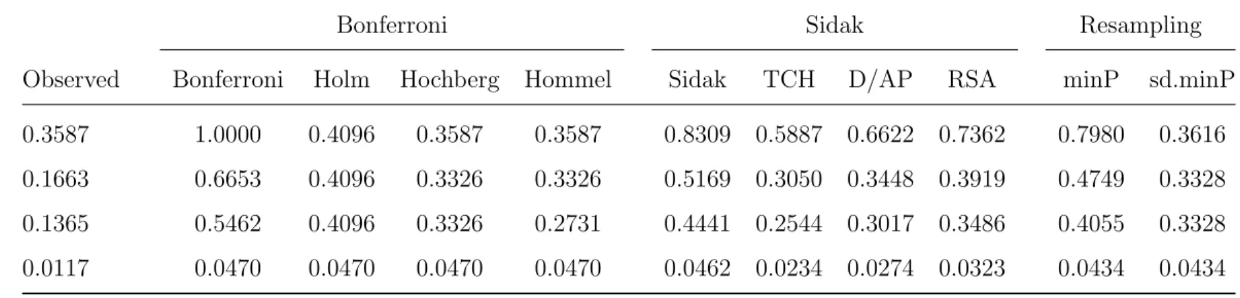
We demonstrate these methods with an illustrative example, with values summarized in Table 2.1. In practice, we would calculate most of these adjusted p-values via efficient com-puter algorithms available in several statistical packages, including R (R Development Core Team, 2008) and SAS/STAT software (SAS Institute Inc., 2002-2006). Suppose we conduct two-sample t-tests with M = 4 outcomes and observe ordered p-values p1 = 0.3587, p2 =
0.1663, p3 = 0.1365, and p4 = 0.0117. Using the Bonferroni method, these unadjusted p-values are each multiplied by 4, producing the values 1.4348, 0.6653, 0.5462, and 0.0470, respectively. By the minimum function, pa1 is set to 1 rather than 1.4348, ensuring adjusted p-values between 0 and 1.
The Holm and Hochberg methods begin by computing the values where jpj, which are
0.3587, 0.3326, 0.4096, and 0.0470. These are potential adjusted p-values, determined ulti-mately by the stepwise procedures. Per the Holm method, we note 0.3326 <0.4096. Since the method requires that pa2 ≥ pa3, we set pa2 = 0.4096, not the initial potential value
0.3326. Similarly, with the requirementpa1 ≥pa2, we setpa1 = 0.4096, resulting in the Holm p-values, 0.4096, 0.4096, 0.4096, and 0.0470. Per the Hochberg method, we again note that 0.3326 < 0.4096, and that the requirement pa2 ≥ pa3 exists. Under the Hochberg method,
we set pa3 = 0.3326 rather than the initial potential value 0.4096, resulting in the Hochberg p-values 0.3587, 0.3326, 0.3326, and 0.0470.
The Hommel method requires the calculation of Simesp-values for subsets of hypotheses for each adjusted p-value. For example, pa3 requires the calculation of Simes p-values for
the following four hypothesis subsets: {H01, H02, H03, H04},{H01, H02, H03},{H01, H03}, and
{H03}. The Simes p-values for these subsets are 0.0470, 0.2495, 0.2731, and 0.1365, where
pa3is the maximum of these values, 0.2731. The Hommelp-values are 0.3587, 0.3326, 0.2731,
and 0.0470.
Table 2.1: Illustrative Example: Observed P-Values and AdjustedP-Values by Class and Method
Bonferroni Sidak Resampling
Observed Bonferroni Holm Hochberg Hommel Sidak TCH D/AP RSA minP sd.minP
0.3587 1.0000 0.4096 0.3587 0.3587 0.8309 0.5887 0.6622 0.7362 0.7980 0.3616 0.1663 0.6653 0.4096 0.3326 0.3326 0.5169 0.3050 0.3448 0.3919 0.4749 0.3328 0.1365 0.5462 0.4096 0.3326 0.2731 0.4441 0.2544 0.3017 0.3486 0.4055 0.3328 0.0117 0.0470 0.0470 0.0470 0.0470 0.0462 0.0234 0.0274 0.0323 0.0434 0.0434
Note. TCH = Tukey-Ciminera-Heyse; D/AP = Dubey/Armitage-Parmar; RSA = R2 adjustment.
The Sidak-class methods have the same general form,paj = 1−(1−pj)g(j). Usingg(j) =
M = 4, the Sidak p-values are 0.8309, 0.5169, 0.4441, and 0.0462. Using g(j) = √M = 2, the TCH p-values are 0.5887, 0.3050, 0.2544, and 0.0234. The D/AP and RSA methods require correlation information. Suppose the values of mean.ρ(j), the mean correlation for thejthoutcome with all other outcomes, are 0.3558, 0.3915, 0.3546, and 0.3841 for outcomes
V(1)-V(4), respectively. Using the D/AP formula, the adjustedp-values are 0.6622, 0.3448, 0.3017, and 0.0274. Similarly, with R2(j) values of 0.2077, 0.2744, 0.2271, and 0.2618, the RSA p-values are 0.7362, 0.3919, 0.3486, and 0.0323.
The resampling-class methods rely on the empirical minP null distributions. We gen-erated the distributions based on Nboot = 100,000 resamples. By the minP method, paj
is the probability of observing a value X ≤ pj, where X follows the empirical minP null
distribution derived using all four outcomes. In a graphical representation, this corresponds to the area under the empirical distribution plot to the left of the value of pj. The minP
p-values based on our generated distribution are 0.7980, 0.4748, 0.4055, and 0.0434. Per the sd.minP method, we compare only p4, the smallestp-value, against this distribution. Recall
that each pj is compared to the distribution derived from using only outcomes B(1)-B(j).
Thus,pa3 is calculated using the distribution based only on B(1)-B(3), and so forth. Based
on these distributions, the potential value for eachpaj is the area to the left ofpj and below
the appropriate distribution curve. These potential values are 0.3616, 0.2925, 0.3328, and 0.0434. Similar to the Holm method, we note 0.2925<0.3328, and thus adjust pa2 upward
to the value of pa3, resulting in sd.minP p-values 0.3616, 0.3328, 0.3328, and 0.0434. We
provide a graphical representation in Figure A1 of the Supplementary Materials.
2.4 SENSITIVITY ANALYSIS
2.4.1 Data
We used a dataset from a study of neuropsychological performance conducted through the University of Pittsburgh’s Advanced Center for Interventions and Services Research for
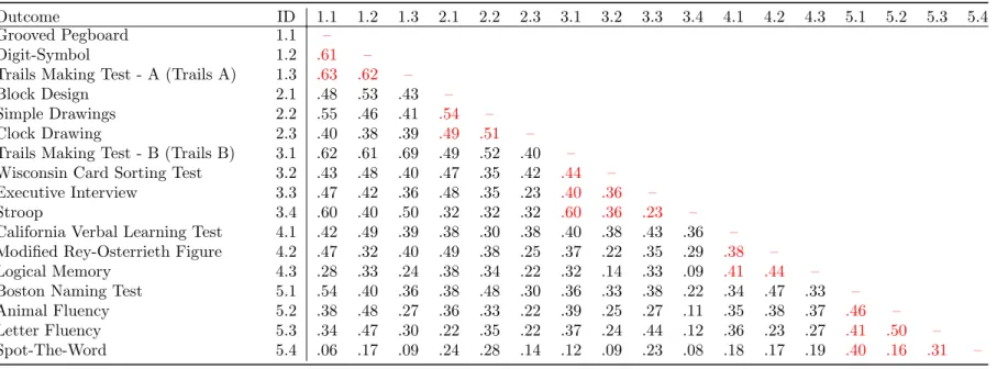
Life Mood Disorders, Western Psychiatric Institute and Clinic in Pittsburgh, PA (Butters et al., 2004). The study used a group of 140 subjects (100 depressed, 40 non-depressed comparison subjects), ages 60 and above, group-matched in terms of age and education. We conducted our sensitivity analysis with respect to 17 interrelated neuropsychological tests (i.e. outcome measures) from this dataset, with tests detailed and cited in Butters et al. These outcome measures were grouped into five theoretical domains. The outcome correlation matrix is shown in Table 2.2
2.4.2 Analysis
The sensitivity analysis was performed to compare the ten adjustment methods, described in the P-Value Adjustment Methods section, with respect to patterns of hypothesis rejection and inference. We conducted two-sample t-tests to test the null hypothesis of no differ-ence between the depressed and comparison groups for each of the 17 outcome measures. The p-value adjustment methods were applied using the multtest procedure, available in the SAS/STAT software (SAS Institute Inc., 2002-2006). This procedure allowed for the computation of adjusted p-values for the Bonferroni- and resampling-class methods, as well as the Sidak method. For the resampling methods, 100,000 bootstrap samples were used in the calculations. The Sidak derivatives (TCH, D/AP, and RSA) were programmed in a SAS macro (available upon request).
2.4.3 Results
Figure2.1 compares the adjustedp-values for each method across all outcomes. The legend indicates the total number of rejected hypotheses per method. We used a square-root scale for the y-axis to reduce the quantity of overlapping points. Adjusted p-values based on the smaller unadjusted p-values, primarily in the information processing speed and visuospatial ability domains, remained difficult to distinguish; the numerical values are shown in Ta-ble A1 in the Supplementary Materials. Among Bonferroni-class methods, the Bonferroni method had the largest p-values, and thus was the most conservative, followed by Holm, Hochberg, and Hommel being the least conservative of the methods. The Sidak method
Table 2.2: Neuropsychological Outcome Correlation Matrix
Outcome ID 1.1 1.2 1.3 2.1 2.2 2.3 3.1 3.2 3.3 3.4 4.1 4.2 4.3 5.1 5.2 5.3 5.4
Grooved Pegboard 1.1 –
Digit-Symbol 1.2 .61 –
Trails Making Test - A (Trails A) 1.3 .63 .62 –
Block Design 2.1 .48 .53 .43 –
Simple Drawings 2.2 .55 .46 .41 .54 –
Clock Drawing 2.3 .40 .38 .39 .49 .51 –
Trails Making Test - B (Trails B) 3.1 .62 .61 .69 .49 .52 .40 –
Wisconsin Card Sorting Test 3.2 .43 .48 .40 .47 .35 .42 .44 –
Executive Interview 3.3 .47 .42 .36 .48 .35 .23 .40 .36 –
Stroop 3.4 .60 .40 .50 .32 .32 .32 .60 .36 .23 –
California Verbal Learning Test 4.1 .42 .49 .39 .38 .30 .38 .40 .38 .43 .36 –
Modified Rey-Osterrieth Figure 4.2 .47 .32 .40 .49 .38 .25 .37 .22 .35 .29 .38 –
Logical Memory 4.3 .28 .33 .24 .38 .34 .22 .32 .14 .33 .09 .41 .44 –
Boston Naming Test 5.1 .54 .40 .36 .38 .48 .30 .36 .33 .38 .22 .34 .47 .33 –
Animal Fluency 5.2 .38 .48 .27 .36 .33 .22 .39 .25 .27 .11 .35 .38 .37 .46 –
Letter Fluency 5.3 .34 .47 .30 .22 .35 .22 .37 .24 .44 .12 .36 .23 .27 .41 .50 –
Spot-The-Word 5.4 .06 .17 .09 .24 .28 .14 .12 .09 .23 .08 .18 .17 .19 .40 .16 .31 –
For ID, x.y indicates the yth outcome of domain x. Domain 1 = Information Processing Speed; Domain 2 = Visuospatial; Domain 3 =
Executive; Domain 4 = Memory; Domain 5 = Language.
0.00 0.05 0.10 0.20 0.30 0.40 0.50 0.60 0.70 0.80 0.90 1.00 Grooved Pegboard Digit−
Symbol Trails A Block Design Simple
Drawings Clock Drawing Trails B WCST EXIT Stroop CVLT Modified Rey− Osterrieth
Logical Memory Boston Naming
Test
Animal Fluency Letter Fluency Spot− The− Word
+ + + + + o + o o x o o o x
Information Processing Speed Visuospatial Executive Memory Language
Adjusted P−Value Outcome Domain ● ● ● ● ● ● ● ● ● ● ● ● ● ● ● ● ● ● ● ● ● ● ● ● ● ● ● ● ● ● ● ● ● ● ● ● ● ● ● ● ● ● ● ● ● ● ● ● ● ● ● ● ● ● Bonferroni−Class Bonferroni (8) Holm (10) Hochberg (10) Hommel (12) Sidak−Class Sidak (8) TCH (12) D/AP (11) RSA (12) Resampling−Class MinP (6) Step−down MinP (7) No Adjustment (14)
Figure 2.1: Adjusted P-Values by Method across Neuropsychological Outcomes
Seventeen observedp-values for a set of 17 neuropsychological measures, and adjustedp-values per each method. A square-root scale is
used to reduce overlapping points. Numbers in parentheses in the legend indicate the number of rejected hypotheses for that method. Symbols for outcomes with a null hypothesis rejected without adjustment indicate the following: + = null hypothesis rejected using
each adjustment method; × = null hypothesis not rejected using any adjustment method; o = hypothesis rejected by some adjustment
methods. Note. WCST = Wisconsin Card Sorting Test, EXIT = Executive Interview, CVLT = California Verbal Learning Test.
Adapted from Table 2 of Butters et al. (2004),Archives of General Psychiatry,61(6), 587–595. Copyright c(2004), American Medical
Association. All rights reserved.
produced similar results to the Bonferroni method. The Sidak derivatives were more liberal, all producing results similar to the Hochberg and Hommel methods; D/AP was most con-servative of the three. Generally, TCH was the least concon-servative, though RSA produced some smaller p-values, mostly when the observedp-value was also quite small.
The resampling methods produced relatively conservative results, with overall inferences similar to the Bonferroni and Sidak methods. The sd.minP method rejected the null hy-pothesis for the Clock Drawing Test, which was not rejected by the Bonferroni or Sidak methods. Whereas the order relations of the Bonferroni- and Sidak-class adjusted p-values were highly consistent, this failed to hold for the resampling-class methods. The adjusted resampling-class p-values were smaller than the Hommel counterpart for some outcomes, and larger than the Bonferroni counterpart for others. Compared against each other, the sd.minP p-values were smaller than the minPp-values.
These results highlight the importance of multiple hypothesis testing. We rejected 14 of the 17 hypotheses without any adjustment. Of these 14, the null hypotheses regarding Animal Fluency and Stroop were not rejected using any p-value adjustment method, sug-gesting the unadjusted hypothesis decisions were Type I errors. Six of these 14 hypotheses were rejected using every method. Though the truth is unknown, the consistency of rejection across methods adds a degree of believability in these decisions. The remaining hypotheses were rejected by varying subsets of the methods. Without knowing the true differences (or lack thereof) between the populations regarding these outcomes, this comparison underscores the need to evaluate and understand the Type I error and power properties of these p-value adjustment methods.
2.5 SIMULATION STUDY
2.5.1 Methods
The premise of the simulation study, conducted using the R statistical package (R Develop-ment Core Team, 2008), was to assess adjustment method performance across two series of
trials. Performance included both Type I error protection and power to detect true effects. We defined each trial by a combination of hypothesis set and correlation structure condi-tions, defined below and summarized in Table 2.3. In a given trial, we generated 10,000 random datasets, termed replicates, with two groups of sizeN = 100 observations each. We chose to generateM = 4 outcome variables, termedV1 through V4, to represent an average neuropsychological domain. Outcomes were generated to follow multivariate normal distri-bution using the mvrnorm function (Venables and Ripley, 2002). Type I error and power estimates were calculated using the method-specific adjustedp-values, based on two-sample, equal-variance, two-sided t-test p-values from each replicate. The number of resampled datasets,Nboot, nontrivially impacts computation time, but has less impact on performance
estimation accuracy compared to the number of replicates (Westfall and Young,1993). We setNboot = 500 for efficiency.
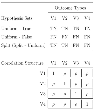
Table 2.3: CS Simulation Series Parameters
Outcome Types
Hypothesis Sets V1 V2 V3 V4
Uniform - True TN TN TN TN Uniform - False FN FN FN FN Split (Split - Uniform) TN TN FN FN
Correlation Structure V1 V2 V3 V4
V1 1 ρ ρ ρ
V2 ρ 1 ρ ρ
V3 ρ ρ 1 ρ
V4 ρ ρ ρ 1
Note. Outcome types: TN = true null; FN = false null; V1-V4 = outcomes 1-4. Compound
symmetry: ρ={0.0,0.1, . . . ,0.9}.
We defined atrue null (TN) as a simulated outcome with no difference between groups. The null hypothesis is actually true, and the p-value for the hypothesis test should be non-significant. True null outcomes were simulated with an effect size of 0.0 between the two groups, and were used for Type I error estimation. We defined a false null (FN) as a simulated outcome with a significant difference between the groups, or alternatively, the null hypothesis is false. False null outcomes were simulated with an effect size of 0.5 between groups, and were used for power estimation. Varying combinations of TNs and FNs, termed hypothesis sets, defined the outcomesV1-V4. The uniform hypothesis sets defined all four outcomes to be the same type, either all true or all false nulls, allowing only Type I error or power estimation, respectively. The split hypothesis set defined two outcomes as TNs, and the other two as FNs, and allows both Type I error and power estimation using the relevant simulated outcomes. These hypothesis sets defined the truth in a given trial, allowing for absolute comparisons of the p-value adjustment methods against the truth instead of only the relative comparisons afforded by the sensitivity analysis.
For all trials, we defined the significance threshold for all p-values at α =.05. We used several performance measures detailed by Dudoit et al. (2003) with adapted nomenclature. Using TN outcomes, we defined Type I error as the family-wise error rate, meaning the probability of rejecting at least one TN hypothesis. We defined minimal power as the probability of rejecting at least one FN hypothesis. We defined maximal power as the probability of rejecting all FN hypotheses. These performance measures were calculated as the proportion of replicates satisfying the respective conditions. We definedaverage power as the average probability of rejecting the FN hypotheses across outcomes. This measure was calculated as the mean proportion of rejected FN hypotheses across outcomes.
To examine the effect of correlation between outcomes on p-value adjustment method performance, we varied the correlation levels in the two simulation series systematically. The first simulation series, the compound-symmetry (CS) series, used a CS correlation structure where all outcomes were equicorrelated with each other. We varied the correlation parameterρ from 0.0-0.9 with an interval of 0.1 for ten possible values. With three specified hypothesis sets (uniform-true, uniform-false, and split) and ten CS structures, 30 trials were conducted in this series, summarized in Table 2.3.
The second simulation series, block-symmetry (BS), defined the outcomes V1-V2 and V3-V4 to constitute Blocks 1 and 2. Outcomes were equicorrelated within and between blocks, but with different levels. Within- and between-block correlation parameters W and B were varied among the values 0.0, 0.2, 0.5, and 0.8 (no, low, moderate, and high correla-tion), where within-block correlation was held strictly greater than between-block correlation, that is, W > B. The correlation structure of the sensitivity analysis data indicated higher correlation magnitude between outcomes within a block (domain) than between outcomes from different blocks. The BS correlation structure allows for the variation of these magni-tudes in a simpler, four-outcome, two-block setting. In addition, the split-split hypothesis set was used, which defined a mix of outcome types overall and within blocks. This differed from the split, or split-uniform, hypothesis set where block-specific hypothesis subsets were uniform. With four hypothesis sets and six correlation structures, 24 trials were conducted in this series. Table A2 in theSupplementary Materials summarizes the BS series parameters. These structures represent correlation patterns observed between outcomes within and across several domains in the sensitivity analysis data. The CS structure is relevant to studies that focus on a single domain, e.g., visuospatial ability, with multiple outcomes, e.g., block design, simple drawings, clock drawing. While less intuitive compared to the CS structure, the BS structure is relevant for studies with multiple domains, e.g., visuospatial ability and memory. While correlation structures of real data are more complicated, these structures provided a relevant and convenient basis for evaluating the p-value adjustment methods.
2.5.2 Results
For brevity, we report the simulation results for the CS series in full. BS series results exhibited similar patterns, and thus, we provide BS series performance results in Figures
A2, A3, and A4 in the Supplementary Materials. We also note the primary purpose of the
p-value adjustment methods is to control Type I error, that is, they maintain Type I error near or belowα =.05. When viewing the power plots, take note of Type I error as well, as methods with power greater than others but with insufficient Type I error control fail the primary purpose and render them suboptimal.
2.5.2.1 Compound-Symmetry - Uniform Hypothesis Set
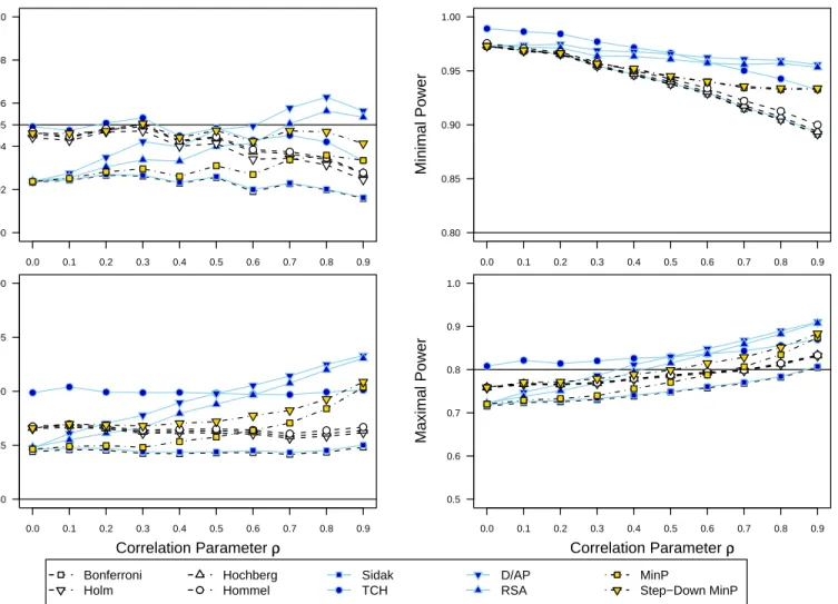
In Figure 2.2, we show the performance across CS correlation structures for the p-value adjustment methods under the uniform hypothesis sets (4 TNs for Type I error, 4 FNs for power). Type I error performance is shown in the upper-left panel. The resampling-class methods demonstrated stable Type I error around α = .05 as the CS correlation ρ increased. The Bonferroni-class methods demonstrated a decreasing trend in Type I error with increasing correlation between outcomes. The Bonferroni and Holm methods showed the lowest Type I error, whereas the Hochberg and Hommel methods allowed more error, but were still conservative when ρ exceeded 0.5. The Sidak method exhibited marginally higher Type I error than the Bonferroni method. The TCH method followed a decreasing, but elevated trend; in the case of independence, it demonstrated high Type I error with values nearly double the threshold α = .05. However, in the case of high correlation, ρ = 0.9, it was the only method that reasonably approached α = .05. The D/AP and RSA methods followed liberal non-monotonic trends. These methods showed increasing Type I error up to point around ρ = 0.6-0.7, after which the trends decreased.
For average power, shown in the lower-left panel, all the methods exhibited acceptable rates >0.8. The Bonferroni and Sidak methods exhibited low, stable power near 0.85. The stepwise Bonferroni derivatives exhibited high power that decreased slowly with increasing correlation. The Hommel method was slightly more powerful than Hochberg, which was more powerful than Holm. The TCH method showed reasonably stable power around 0.9. The D/AP and RSA methods increased in average power asρ increased, and at high correlation, were more powerful than the Bonferroni derivatives. However, as noted before, the power for the Sidak derivatives is irrelevant considering the Type I error rates well aboveα=.05. The minP method showed an increasing trend in average power with increasing correlation. The sd.minP method demonstrated an increase in power associated with a stepwise approach.
For minimal power, shown in the upper-right panel, all methods were able to detect a difference between groups for at least one of four outcomes across all correlations with power > 0.9. The original Bonferroni and Sidak methods had the least power, followed by the Bonferroni derivatives, the resampling-class methods, and finally the Sidak derivatives.
● ● Bonferroni Holm Hochberg Hommel Sidak TCH D/AP RSA MinP Step−Down MinP Type I Error 0.00 0.02 0.04 0.05 0.06 0.08 0.10 0.0 0.1 0.2 0.3 0.4 0.5 0.6 0.7 0.8 0.9 ● ● ● ● ● ● ● ● ● ● ● ● ● ● ● ● ● ● ● ● Average Power 0.80 0.85 0.90 0.95 1.00 Correlation Parameter ρρ 0.0 0.1 0.2 0.3 0.4 0.5 0.6 0.7 0.8 0.9 ● ● ● ● ● ● ● ● ● ● ● ● ● ● ● ● ● ● ● ● Minimal Power 0.80 0.85 0.90 0.95 1.00 0.0 0.1 0.2 0.3 0.4 0.5 0.6 0.7 0.8 0.9 ● ● ● ● ● ● ● ● ● ● ● ● ● ● ● ● ● ● ● ● Maximal Power 0.5 0.6 0.7 0.8 0.9 1.0 Correlation Parameter ρρ 0.0 0.1 0.2 0.3 0.4 0.5 0.6 0.7 0.8 0.9 ● ● ● ● ● ● ● ● ● ● ● ● ● ● ● ● ● ● ● ●
Figure 2.2: P-Value Adjustment Method Performance across Compound-Symmetry Correlation Structures Type I Error and Power Estimates for Uniform Hypothesis Set
The upper-left panel shows Type I error rates of thep-value adjustment methods across increasing values of the CS correlation parameter
ρ. In this case, all M = 4 hypotheses are simulated to be true. Values near α = .05 are optimal. Values well above α =.05 indicate
failure to protect Type I error atα. The remaining panels show different measures of power, where the 4 hypotheses are simulated to be
false. Higher power is optimal, conditional upon Type I error not exceedingα.
For maximal power, shown in the lower-right panel, all methods exhibited less power in comparison to the minimal and average power, and demonstrated monotonic increasing trends with higher correlation with differing rates of change. The Bonferroni and Sidak methods again demonstrated the least power. The Bonferroni derivatives and the sd.minP performed generally well, ranging from just below 0.8 for low correlation and approach 0.9 for high correlation. As before, Holm was less powerful than Hochberg, which was equivalent to Hommel, with the sd.minP method inbetween. Again, the TCH method followed the Sidak pattern in an elevated fashion. The D/AP and RSA methods demonstrated a steep rate of increase with increasing correlation, with power levels near Sidak with low correlation, and power similar to the Bonferroni derivatives and the sd.minP method at high correlation.
2.5.2.2 Compound-Symmetry - Split Hypothesis Set
Figure 3 shows the results for the split hypothesis set across compound-symmetry correlation structures. Similar relationships were found in comparison to the uniform hypothesis set, though the overall magnitudes decreased for all methods. Of note is the relative lack of decrease seen among stepwise methods, the Bonferroni derivatives and the sd.minP methods. The Type I error rates of the other methods were nearly halved in many instances. The D/AP and RSA methods exceeded α =.05 for high values of ρ.
Compared to the uniform hypothesis set power estimates, the Bonferroni derivatives exhibited lower average power, whereas the other methods performed similarly. The sd.minP method also showed a decrease in average power, though it increased with correlation. For minimal power, all methods exhibited a small reduction in power, though less pronounced for the Sidak derivatives. In terms of maximal power, the results for the Bonferroni derivatives were similar to the uniform hypothesis set counterparts, and all other methods exhibited greater power. The Bonferroni and Sidak methods continued to be the most conservative, but the Sidak derivatives exhibited higher power than all other methods for CS correlation ρ >0.3.
● ● Bonferroni Holm Hochberg Hommel Sidak TCH D/AP RSA MinP Step−Down MinP Type I Error 0.00 0.02 0.04 0.05 0.06 0.08 0.10 0.0 0.1 0.2 0.3 0.4 0.5 0.6 0.7 0.8 0.9 ● ● ● ● ● ● ● ● ● ● ● ● ● ● ● ● ● ● ● ● Average Power 0.80 0.85 0.90 0.95 1.00 Correlation Parameter ρρ 0.0 0.1 0.2 0.3 0.4 0.5 0.6 0.7 0.8 0.9 ● ● ● ● ● ● ● ● ● ● ● ● ● ● ● ● ● ● ● ● Minimal Power 0.80 0.85 0.90 0.95 1.00 0.0 0.1 0.2 0.3 0.4 0.5 0.6 0.7 0.8 0.9 ● ● ● ● ● ● ● ● ● ● ● ● ● ● ● ● ● ● ● ● Maximal Power 0.5 0.6 0.7 0.8 0.9 1.0 Correlation Parameter ρρ 0.0 0.1 0.2 0.3 0.4 0.5 0.6 0.7 0.8 0.9 ● ● ● ● ● ● ● ● ● ● ● ● ● ● ● ● ● ● ● ●
Figure 2.3: P-Value Adjustment Method Performance across Compound-Symmetry Correlation Structures Type I Error and Power Estimates for Split Hypothesis Set
The upper-left panel shows Type I error rates of thep-value adjustment methods across increasing values of the CS correlation parameter
ρ. In this case, all only 2 of the M = 4 hypotheses are simulated to be true. Values nearα=.05 are optimal. Values well above α=.05
indicate failure to protect Type I error atα. The remaining panels show different measures of power, using the two hypotheses simulated
to be false. Higher power is optimal, conditional upon Type I error not exceedingα.
2.6 DISCUSSION
The simulation results indicated that the Bonferroni and Sidak methods, while protecting Type I error, became increasingly conservative with high correlation between outcomes, and were underpowered, particularly with regard to maximal power. The Bonferroni derivatives, while not improving the Type I error issue, notably improved average and maximal power. The single-step Sidak derivatives did not exhibit power similar to the stepwise methods. The average power of the D/AP and RSA methods increased with increasing correlation. How-ever, these methods did not maintain acceptable Type I error. The resampling-class methods demonstrated consistent Type I error across the correlation structures and levels explored. The sd.minP method again demonstrated the advantage of a stepwise approach with similar power to the Bonferroni-derivatives. Among methods examined, the Hochberg, Hommel, and sd.minP methods exhibited the best performance, with considerable power and reasonable Type I error protection. With higher outcome correlation, the sd.minP method demonstrated higher power, particularly in the split hypothesis experiments. Thus, for lower correla-tion between neuropsychological outcomes, i.e. average ρ <0.5, we recommend either the Hochberg or Hommel methods for reasons of easy implementation and exact replicability. For higher correlation between neuropsychological outcomes, we recommend the sd.minP method for increased power.
However, we must note a caveat to this simple guideline. With the implementation of the SAS/STAT multtest procedure (SAS Institute Inc., 2002-2006), the equal-variance assumption was the only option for the test statistics used with the minP and sd.minP methods. When the equal-variance assumption is violated, using equal-variancet-tests may yield inaccurate observed p-values and inaccurate empirical minP null distributions, thus producing the conservative results shown in our sensitivity analysis.
Ideally, one might wish to use the sd.minP method without assuming equal variances for all outcomes, though to our knowledge, current statistical software packages do not support this feature. Whereas the parametric methods are simple formulae that produce identical results across packages, the resampling-class methods may vary in their implementation from package to package, specifically with respect to the Type of tests that may be conducted. If
equality-of-variance tests are rejected for many outcomes, current software implementations may yield lower power. In this case, for averageρ≥0.5, we prefer the Hochberg and Hommel methods. For the neuropsychological data examined in the sensitivity analysis, with high correlation between outcomes and many outcomes with unequal variances between groups, the Hochberg and Hommel methods are most appropriate.
Another important caveat with regard to the resampling-class methods is the number of Nboot samples used to generate the empirically-derived null minimum p-value
distribu-tions. Westfall and Young (1993) recommend at least 10,000. In practice, this may not be enough. One cannot estimate small p-values with a reasonable amount of precision without enough samples to estimate the tails of the distribution. With too few resamples, repeated applications of these methods may yield different inferences. While we used 100,000 for our sensitivity analysis, admittedly, the smallest unadjusted p-value could not have been pre-cisely estimated with 100,000, though the adjusted counterpart was still quite belowα=.05. The D/AP and RSA methods, designed to incorporate correlation into the adjustment, proved insufficient in protecting Type I error. The average power of these methods was adequate, but maximal power was weak for low correlation between outcomes. Further research in this area may yield another function that overcomes these deficiencies.
More methods may have been considered in this investigation. Dunnett and Tamhane
(1992) and Rom (1990) both developed stepwise procedures with the motivation of lowering Type II error. Both methods make strong distributional assumptions and require compli-cated, iterative calculation. Furthermore, neither method has been implemented in any statistical software. The resampling-class methods also include permutation methods, which yield similar results to bootstrap methods when both methods can be easily applied, but are extremely complicated to apply in many analytical situations (Westfall and Young, 1993). Thus, we excluded these methods from consideration.
We chose to simulate only four outcomes to obtain a perspective of the performance of these methods. It is likely that the trends would simply become more pronounced and exaggerated with a higher number of outcomes, though this could be confirmed by another extensive simulation study.
The sensitivity analysis and simulation study were conducted in SAS and R as many of the methods used were built into the software and the remaining methods could be pro-grammed with relative ease. SPSS and Stata, software preferred by some researchers, have a limited selection of methods available for ANOVA-type comparisons, and none for multi-ple, two-sample tests as explored in this study (SPSS Inc., 2006; Stata Press, 2007). The Hochberg method could be programmed with relative ease in either package; in fact, it could be programmed in spreadsheet software. The Hommel and sd.minP methods, however, would be more complicated. Reprogramming these methods for SPSS or Stata would likely be less efficient than learning the comparatively few commands necessary to conduct the p-value adjustments in SAS or R.
Currently, there exists no perfect adjustment method for multiple hypothesis testing with neuropsychological data. The sd.minP, Hochberg, and Hommel methods demonstrated Type I error protection with good power, though new research may yield methods that surpass their performance.
2.7 ACKNOWLEDGEMENTS
This research was supported by the National Institute of Mental Health (NIMH) T32 MH073451, the NIMH P30 MH071944, the NIMH R01 MH072947, and the National Institute on Aging P01 AG020677. We thank Dr. Sanat Sarkar of Temple University for his input for this manuscript.
3.0 CONSIDERING P-VALUE DEPENDENCE IN A STEPWISE MULTIPLE TESTING PROCEDURE
Richard E. Blakesley, BS 1
1 Department of Biostatistics, University of Pittsburgh
Manuscript in Progress
3.1 ABSTRACT
Controlling the familywise error rate (FWER) with correlated outcome variables has proven challenging. Several parametric multiple testing procedures (MTPs) control the FWER under independence, but have shown conservative FWER control when independence is vi-olated. Nonparametric, resampling-based MTPs have demonstrated FWER control with good power, regardless of outcome correlation, though implementation can be an obstacle. The Dubey/Armitage-Parmar and R2 Adjustment methods, parametric MTPs that
incor-porate correlation information, have demonstrated unstable FWER protection. We propose a parametric MTP to address issues of the existing MTPs to control the FWER with corre-lated outcomes. We conducted a simulation study to estimate the FWER and power of the proposed method and selected existing MTPs across many combinations of simulation trial parameters, with a desired FWER α= 0.05. The proposed and the step-down minP meth-ods demonstrated similar FWER and power estimates across the conditions explored, with power equal to or exceeding the Hochberg and Hommel methods under moderate to high correlation conditions. Similar relative patterns were seen in a microarray dataset example. While not proven to control FWER in a theoretical context, the proposed parametric method has exhibited, through simulation, the desired properties of a multiple testing procedure.
Key words: multiple hypothesis testing, multiple testing procedure, multiple compar-isons, multiplicity adjustment, adjusted p-value, correlated outcomes, familywise error rate
3.2 INTRODUCTION
Multiplicity refers to the increasing risk of rejecting incorrectly null hypotheses, Type I errors, as the number of hypothesis tests increases (Pocock, 1997). This problem arises when conducting several hypothesis tests, such as two-samplet-tests with respect to multiple outcome variables, or multiple analysis of variance contrasts. A specific measure of Type I error is the familywise error rate (FWER), the probability of rejecting incorrectly one or more null hypothesis. When multiplicity is present, e.g., neuropsychological and genetic studies, failure to control the FWER may yield questionable results.
Blakesley et al. (in press) performed a simulation study examining ten multiple test-ing procedures (MTPs), grouped into three classes. Bonferroni-class methods include the Bonferroni method (Simes, 1986) and its derivatives, the stepwise methods developed by
Holm (1979), Hochberg(1988), andHommel (1988). Sidak-class methods include the Sidak method (Sidak, 1967) and its derivatives, which include the Tukey-Ciminera-Heyse (TCH), Dubey/Armitage-Parmar (D/AP) and R2 adjustment (RSA) methods (Sankoh et al.,1997).
Resampling-based methods include the minP and step-down (SD) minP methods (Westfall and Young, 1993). Blakesley et al. identified three methods that performed well in their simulation, though with caveats. While the SD minP method performed the best, it suffered from computation and implementation issues. The Hochberg and Hommel methods, though simpler to implement, trended conservative with increasing correlation coefficients between outcomes.
Ideally, an MTP should maintain stable FWER control at a desired critical value, α, meaning an MTP should not be more conservative or liberal depending on the number of hypotheses, the true statuses of the null hypotheses, and the level of correlation between outcomes. Also, an MTP should maintain adequate power to detect real effects by rejecting hypotheses that are actually false. In Section3.3, we propose a parametric MTP to achieve these ideal MTP characteristics, in the context of existing methods. In Sections3.4 and 3.5, we detail the design and results of the simulation study conducted to examine the FWER and power rates of the proposed and existing methods. We demonstrate these MTPs with a real data example in Section 3.6. Finally, we discuss our findings in Section 3.7.
3.3 MULTIPLE TESTING PROCEDURES
3.3.1 Notation
We denote the set of observedp-values,{pm}, with themthp-valuepm corresponding to null
hypothesisHm and outcomeXm, m∈ {1, . . . , M}. We partitionXm =
X1m X2m N×1 such
that Xam = {Xabm}n×1, a∈ {1,2}, b ∈ {1, . . . , n}, N = 2n. We denote the counterpart
set of ordered p-values, p(m) , where p(m) is the mth largest observed p-value in {pm}.
That is, p(1) ≥ p(2) ≥ . . . ≥ p(M). We denote the mth ordered null hypothesis H(m) and
ordered outcome X(m) corresponding to p(m). For a given MTP, we denote the sets of
adjusted observed p-values, {pem}, and adjusted ordered p-values,
e
p(m) . We define the
MTPs in terms of the adjusted orderedp-values; adjusted observed p-values are determined by resorting the adjusted ordered p-values by the original order.
3.3.2 Parametric FWER Control with Independent P-Values
Under the null hypothesis, we assume eachpm ∼i.i.d. U (0,1), thus we assume the minimum
p-value min
1≤m≤M pm =p(M) ∼Beta(1, M) with the CDF defined by the regularized incomplete
beta function, Ix(1, M). Comparing each pm againstα, we define the FWER as:
P [any pm ≤α] =P min 1≤m≤M pm ≤α =Iα(1, M) = M X j=1 M j αj(1−α)M−j = M X j=0 M j αj(1−α)M−j− M 0 α0(1−α)M = 1−(1−α)M (3.1) 33
Alternatively: P [any pm ≤α] = 1−P[all pm > α] = 1− M Y j=1 (1−α) = 1−(1−α)M (3.2)
Thus, controlling individual hypothesis tests atαinflates the FWER, which approaches 1 as M increases. The FWER is controlled at α by comparing hypothesis test p-values against an adjusted α-value, α. Per the method ofe Sidak (1967), we calculate:
e
α=Iα−1(1, M) = 1−(1−α)M1
(3.3)
Equivalent to comparing the observed (or ordered) p-values against the adjustedα-value, α,e one can compare adjusted p-values against the desired FWER α. Using the Sidak method, we calculate adjusted ordered p-values as:
e
p(m) = 1− 1−p(m) M
(3.4)
Relaxing the assumption of uniform p-values, the Bonferroni method adjusts p-values using a simpler formula:
e
p(m) =M p(m) (3.5)
It can be shown that the Bonferroni and Sidak methods produce similar results for small
p-values, as the Bonferroni adjusted p-value is the first term of a Taylor series expansion of the Sidak formula (Westfall and Young,1993).
These methods are categorized assingle-step (SS) methods, which apply the same level of adjustment to allp-values. In contrast,stepwise methods apply differing levels of adjustment to each ordered p-value, followed by a monotonicity-enforcing procedure. Deriving from the