Volume 12 | Issue 1
Article 26
5-1-2013
Fitting Proportional Odds Models to Educational
Data with Complex Sampling Designs in Ordinal
Logistic Regression
Xing Liu
Eastern Connecticut State University, [email protected]
Hari Koirala
Eastern Connecticut State University
Follow this and additional works at:
http://digitalcommons.wayne.edu/jmasm
Part of the
Applied Statistics Commons
,
Social and Behavioral Sciences Commons
, and the
Statistical Theory Commons
This Regular Article is brought to you for free and open access by the Open Access Journals at DigitalCommons@WayneState. It has been accepted for inclusion in Journal of Modern Applied Statistical Methods by an authorized administrator of DigitalCommons@WayneState.
Recommended Citation
Liu, Xing and Koirala, Hari (2013) "Fitting Proportional Odds Models to Educational Data with Complex Sampling Designs in Ordinal Logistic Regression,"Journal of Modern Applied Statistical Methods: Vol. 12: Iss. 1, Article 26.
Sampling Designs in Ordinal Logistic Regression
Cover Page Footnote
Previous versions of this paper were presented at the Modern Modeling Methods Conference in Storrs, CT (May, 2012), the Northeastern Educational Research Association Annual Conference in Rocky Hill, CT (Oct., 2012), and 2013 Annual Meeting of American Educational Research Association (AERA), San Francisco, CA (April, 2013)
This regular article is available in Journal of Modern Applied Statistical Methods:http://digitalcommons.wayne.edu/jmasm/vol12/ iss1/26
235
Fitting Proportional Odds Models to Educational Data
with Complex Sampling Designs in Ordinal Logistic Regression
Xing Liu
Hari Koirala
Eastern Connecticut State University, Willimantic, CT
The conventional proportional odds (PO) model assumes that data are collected using simple random sampling by which each sampling unit has the equal probability of being selected from a population. However, when complex survey sampling designs are used, such as stratified sampling, clustered sampling or unequal selection probabilities, it is inappropriate to conduct ordinal logistic regression analyses without taking sampling design into account. Failing to do so may lead to biased estimates of parameters and incorrect corresponding variances. This study illustrates the use of PO models with complex survey data to predict mathematics proficiency levels using Stata and compare the results of PO models accommodating and not accommodating survey sampling features.
Key words: Ordinal logistic regression, PO models, complex survey designs, linearization, standard errors, single sampling unit, Stata.
Introduction
Ordinal logistic regression is an extension, or a special case, of binary logistic regression when an ordinal outcome variable has more than two levels. The three commonly known models for an ordinal outcome variable include the proportional odds (PO) model, the continuation ratio (CR) model and the adjacent category (AC) logistic regression model, depending on different comparisons among the categories of the response variable. Compared to the other two models, the PO model is the most popular
Xing Liu, Ph.D., is an Associate Professor of Research and Assessment in the Education Department at Eastern Connecticut State University. His research interests include educational assessment, categorical data analysis, longitudinal data analysis and multilevel modeling. Email him at: [email protected]. Hari Koirala, Ph.D., is Professor in the Education Department at Eastern Connecticut State University. His research interests include mathematics education and assessment. Email him at: [email protected].
(Agresti, 1996, 2002, 2007, 2010; Anath & Kleinbaum, 1997; Armstrong & Sloan, 1989; Hardin & Hilbe, 2007; Hilbe, 2009; Liu, 2009; Long, 1997; Long & Freese, 2006; McCullagh, 1980; McCullagh & Nelder, 1989; O’Connell, 2000, 2006; O’Connell & Liu, 2011; Powers & Xie, 2000). The PO model is widely implemented as the default for ordinal regression analysis in general-purpose statistical software packages, such as SAS, SPSS, Stata, S-Plus and R. The PO model estimates the relationship between a set of predictor variables and an ordinal outcome variable via a logit link function. It is also known as the cumulative logit model, because it estimates the cumulative odds of being at or below a particular level of the response variable. In addition, for each predictor variable the estimated cumulative odds are assumed to be the same across all the ordinal categories, thus it is known as the proportional odds assumption.
The conventional PO model assumes that data are collected using simple random sampling by which each sampling unit has an equal probability of being selected from a population. In addition to simple random sampling, researchers also use more complex sampling techniques, such as stratified sampling and multistage cluster sampling. The National
236
Center for Education Statistics (NCES) sponsored and conducted a series of studies, such as the Early Childhood Longitudinal Study-Kindergarten (ECLS-K), National Educational Longitudinal Study of 1988 (NELS:88), and Educational Longitudinal Study of 2002 (ELS:2002), all of which applied complex sampling survey designs. These designs had the common features of using strata, clusters and unequal probability of selection in data collection.Because complex survey sampling designs involve the use of different strata (e.g., geographic areas), clustered sampling techniques and unequal selection probabilities, it is inappropriate to conduct the PO model analysis for the ordinal response variable without taking the survey sampling designs into account. Failing to do so may lead to biased estimates of parameters, incorrect variance estimates and misleading results. Therefore, it is critical for researchers to understand techniques for analyzing data with complex sampling designs.
Although multilevel modeling is a valuable tool for analyzing complex sampling survey data, it is mainly used for model-based analysis (Hahs-Vaughn, 2005; Thomas & Heck, 2001) when data structures are nested or hierarchical (O’Connell & McCoach, 2008; Raudenbush & Bryk, 2002). When the data structure only has a single level, researchers need to identify other appropriate methods which take complex sampling design features into account. Analysis that considers these design features is termed the design-based analysis (Lee & Forthofer, 2006; Levy & Lemeshow, 2008), compared to the model-based analysis (e.g., multilevel analysis). Although several strategies were commonly used for design-based analysis of survey data, using specialized software to accommodate complex sampling designs was the most desirable choice (Hahs-Vaughn, 2005; Thomas & Heck, 2001). Among a few statistical software packages that can perform statistical analyses within the context of survey sampling designs, Stata is a well-known statistical package and is capable of performing numerous statistical analyses for
complex survey data with its svy prefix
command (StataCorp, 2007, 2009, 2011).
Various methods of incorporating weights and design effects in statistical models, such as multiple regression (Hahs-Vaughn, 2005, 2006; Thomas & Heck, 2001), and structural equation modeling (Hahs-Vaughn & Lomax, 2006; Muthen & Setorra, 1995; Stapleton, 2002, 2006, 2008) have been proposed and examples were illustrated. However, the use of complex sampling designs in ordinal logistic regression analysis is scarce. In addition, although researchers are increasingly interested in conducting secondary data analysis using large-scale datasets, the lack of analytic skills makes the task intimidating. Therefore, it is imperative to help educational researchers better understand the ordinal logistic regression model with complex sampling data and utilize it in practice. This study illustrates the use of ordinal logistic regression models with complex survey data to predict mathematics proficiency levels using Stata and compares the results of PO models accommodating and not accommodating survey sampling features, such as stratification, clustering and weights. This article extends previous research which focused on different types of conventional ordinal logistic regression models (Liu, 2009; Liu, O’Connell, & Koirala, 2011, Liu & Koirala, 2012).
For demonstration purposes, ordinal regression analyses were based on data from the Educational Longitudinal Study (ELS): 2002, in which the ordinal outcome of students’ mathematics proficiency was predicted from a set of variables in students’ effort, such as, students can get no bad grades if they decide not to, they keep studying even if material is difficult, and they do best to learn.
Theoretical Framework: The Proportional Odds Model
In binary logistic regression, the outcome variable is dichotomous, with 1 = success or experiencing an event and 0 = failure or not experiencing the event. This model estimates the log odds of the outcome or the probability of success from a set of predictors. The logistic regression model (Menard, 1995) is:
237
( )
( )
( )
( )
1 1 2 2 p p ln logit ln 1 X X X Y x x x ′ = π π = − π = α + β + β +…+ β (1) where logit [π(x)] is the log odds of success, and the odds is a ratio between the probability of having an event and the probability of not having that event.When the outcome variable has more than two levels and is ordinal, the ordinal logistic regression model estimates the odds and the probabilities of being at or below a particular category. The ordinal regression model can be expressed on the logit scale as follows (Liu, 2009):
( )
( )
( )
j j j j j 1 1 2 2 p pln(Y ) logit [
x ]
x
=ln
1
x
(
X
X
X ),
′ =
π
π
− π
= α + −β
−β
−…−β
(2) where πj(x) = π(Y≤j|x1,x2,…xp), which is theprobability of being at or below category j, given a set of predictors. j =1, 2, …, J−1. αj are the cut
points, and β1, β2, …, βp are logit coefficients.
This PO model estimates different cut points, but the effect of any predictor is assumed to be the same across these cut points. Therefore, for each predictor only one logit coefficient is estimated. The proportional odds assumption can be assessed by the Brant test (Brant, 1990), which provides the omnibus test for the overall models and the univariate test for each predictor. To estimate the cumulative odds of being at or
below the jth category, this model can be
rewritten as:
(
)
(
(
1 2 p)
)
1 2 p 1 2 p j 1 1 2 2 p p π Y j|x , x ,...x logit Y j x , x ,...,x ln π Y j|x , x ,...x ( X X X ) ≤ π ≤ = > = α + −β −β −…−β (3)where logit is the log odds of being at or below a particular category relative to being beyond that category. By exponentiating the cumulative logits, we obtain the cumulative odds of being at or below the jth category. The PO model includes
a series of binary logistic regression models where the ordinal response variable is dichotomized while assuming the estimated logit coefficients are the same across these binary models.
Researchers should be aware that software packages may use different forms to express the ordinal logistic regression model and parameterize it differently (Liu, 2009). For example, unlike Stata and SPSS, which both follow the above equation; SAS does not negate the signs before logit coefficients in the equation. To estimate cumulative odds of being at or below a particular category, the SAS PROC LOGISTIC procedure can be used with the ascending option, while the descending option can be applied to the same procedure to estimate the odds of being beyond a particular category. Theoretical Framework: Variance Estimation in Complex Survey Sampling
Two techniques are widely used for unbiased variance estimation in complex sampling survey designs, including linearization and replicated sampling methods (Lee & Forthofer, 2006; Levy & Lemeshow, 2008; Lohr, 1999). The linearization method is the Taylor series approximation, also known as the delta method (Kalton, 1983); while the replicated methods estimate variance of a parameter by generating replicated subsamples and examining the variability of the subsample estimates. The replicated methods, also referred to as resampling methods, include the balanced repeated replication (BRR), the jackknife repeated replication (JRR) and the bootstrap method (Lee & Forthofer, 2006; Levy & Lemeshow, 2008). This article focuses on the Taylor series approximation method because it is implemented as the default in general purpose software packages, such as Stata, SAS, SPSS (Complex Samples Add-on Module) and in specialized software, such as SUDAAN, and AM.
238
The general Taylor series linearization is expressed as (Lee & Forthofer, 2006; Levy & Lemeshow, 2008):...
!
2
)
)(
(
)
)(
(
)
(
)
(
x
=
f
a
+
f
'a
x
−
a
+
f
''a
x
−
a
2+
f
(4) where f′ and f″ are the first and second derivatives of the function, f(x) at a. In statistics, the Taylor series linearization is used to obtain a linear approximation to the nonlinear function or statistic and then the variance of the function or statistic can be derived from the Taylor series approximation.Specifically, the variance estimation in complex survey sampling using the Taylor series expansion follows two steps. First, use the first-order Taylor series to obtain a linear approximation of the function. Second, estimate the variance of the parameter including complex survey features, such as strata, cluster and weight variables. Thus, the variance estimate is a weighted combination of the variance across primary sampling units (PSUs) within a stratum (Lee & Forthofer, 2006). In statistical software packages it is necessary to specify strata, cluster and weights before fitting a statistical model.
To estimate sampling variance of a parameter estimate in ordinal logistic regression, Binder (1983) developed a general formula for linear regression and generalized linear models with the complex survey data using the Taylor series, which is widely used and known as the sandwich variance estimator. In the sandwich form, the middle variance-covariance matrix of the weighted score function is multiplied at both the left and right sides by the inverse of the matrix of second derivatives with respect to the parameter estimate (Binder, 1983; Heeringa, West, & Berglund, 2010).
Methodology Sample
The base-year data from the Educational Longitudinal Study (ELS) of 2002 was used for the analyses. This study, conducted by the National Center for Education Statistics (NCES), longitudinally followed students from
10th grade to their postsecondary school
education and/or even in their work. ELS used a two-stage sampling design (Ingels, et al., 2004; 2005). First, using a stratified sampling strategy, 1,221 eligible public and private schools were selected from a population of approximately 25,000 schools with 10th grade students: of the
eligible schools (clusters), 752 agreed to participate in the study. Second, in each of the schools, approximately 25 students in 10th grade
were randomly selected from the enrollment list. The outcome variable of interest was students’ mathematics proficiency levels in high school, which was an ordinal categorical variable with five levels (1 = capable of doing simple arithmetical operations on whole numbers; 2 = capable of doing simple operations with decimals, fractions, powers and root; 3 = capable of doing simple problem solving; 4 = understanding intermediate-level mathematical concepts and/or finding multi-step solutions to word problems; and 5 = capable of solving complex multiple-step word problems and/or understanding advanced mathematical material) (Ingels, et al., 2004, 2005). Those students who failed to pass through level 1 were assigned to level 0. Table 1 provides the frequency of six mathematics proficiency levels (Liu, & Koirala, 2012).
Data Analysis
First the PO model was fitted without considering the complex sampling designs using the Stata ologit command. Stata SPost (Long & Freese, 2006) package was used to examine the fit statistics and the PO assumption. The same PO model was then fitted with Stata ologit with weights. Finally, svy, the Stata’s survey data command was used to fit the PO model taking all the elements of survey design features, such as strata, cluster and weight variables into account. Before using the svy prefix command, the svyset command was employed to specify the complex sampling design features; the svy: ologit command was then used to conduct the subsequent ordinal regression analysis.
When a stratum contains only a single sampling unit, standard errors of the parameters are estimated to be missing. To deal with this issue, three singleunit() options (i.e., certainty, scaled and centered) were specified separately in the svyset command and the estimated standard
239
errors from each of the three PO models were examined. The Taylor series approximation linearization method, which is the default method in Stata, was used to estimate the sampling variance. The results of the PO models accommodating and ignoring complex sampling designs were compared.Results
Proportional Odds Model with Three Explanatory Variables without Weights
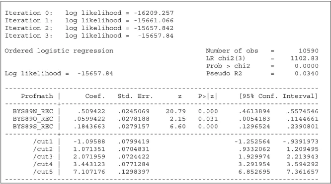
A PO model with all three predictor variables was fitted first. Stata ologit command was used for model fitting. Figures 1 and 2 show the results for the PO model without weights (Unweighted).
The log likelihood ratio chi-square test, LR χ2
(3) = 1102.83, p < 0.001, indicated that the
model with three predictors provides a better fit than the null model with no independent variables. The likelihood ratio, R2
L = 0.034,
suggested that the relationship between the
response variable, mathematics proficiency and the predictors was small.
All logit effects of the three predictors on the mathematics proficiency level were significant. The estimated logit regression coefficient for getting no bad grades if deciding to (decide), β = 0.509, z = 20.79, p < 0.001; the logit coefficient for keeping studying if material is difficult (keeplrn), β = 0.060, z = 2.15, p = 0.0311; and finally, for doing best to learn (dobest), β = 0.184, z = 6.60, p < 0.001.
To estimate the cumulative odds of being at or below a certain mathematics proficiency level, it is only necessary to substitute the values of the estimated logit coefficients into the equation (3). For the first predictor, decide, logit [π(Y≤ j | X1)] =
αj+ (−.509X1). OR = e(-.509) = .601, suggesting
that the odds of being at or below a particular proficiency level decreased by a factor of 0.601 with a one unit increase in the value of the predictor variable, getting no bad grades if Table 1: Proficiency Categories and Frequencies (Proportions)
for the Study Sample, ELS (2002) (N = 15,976) Proficiency
Category Description
Frequency (%)
0 Did not reach level 1 (5.27%) 842
1 Capable of doing simple arithmetical operations on whole numbers (24.30%) 3,882
2 Capable of doing simple operations with decimals, fractions, powers and root (21.42%) 3,422
3 Capable of doing simple problem solving (28.30%) 4,521
4
Understanding intermediate-level mathematical concepts and/or finding multi-step solutions to word problems
3,196 (20.01%) 5
Capable of solving complex multiple-step word problems and/or understanding
advanced mathematical material
113 (0.71%)
240
deciding to, holding others constant. In other words, students were more likely to be in a higher proficiency level with the increase of the frequency in the predictor, getting no bad grades if deciding to. The odds of being at or below a proficiency level for the other two predictors,keeplrn and dobest, were computed in the same way and they were 0.942 and 0.832, respectively.
The odds of being beyond a category of mathematics proficiency are the inverse of those
of being at or below a category. In equation (3), it is necessary to reverse the sign before the logit coefficients and take the exponential of the positive coefficients. All three predictors were positively associated with the odds of being beyond a proficiency level. In terms of odds ratio (OR), the odds of being beyond a proficiency level were 1.664 times greater with one unit increase in the frequency of getting no bad grades if deciding to, 1.062 times greater with one unit increase in the frequency of Figure 1: Stata Proportional Odds Model with Three Explanatory Variables without Weights
Iteration 0: log likelihood = -16209.257 Iteration 1: log likelihood = -15661.066 Iteration 2: log likelihood = -15657.842 Iteration 3: log likelihood = -15657.84
Ordered logistic regression Number of obs = 10590 LR chi2(3) = 1102.83 Prob > chi2 = 0.0000 Log likelihood = -15657.84 Pseudo R2 = 0.0340 --- Profmath | Coef. Std. Err. z P>|z| [95% Conf. Interval] ---+--- BYS89N_REC | .509422 .0245069 20.79 0.000 .4613894 .5574546 BYS89O_REC | .0599422 .0278188 2.15 0.031 .0054183 .1144661 BYS89S_REC | .1843663 .0279157 6.60 0.000 .1296524 .2390801 ---+--- /cut1 | -1.09588 .0799419 -1.252564 -.9391973 /cut2 | 1.071351 .0704831 .9332062 1.209495 /cut3 | 2.071959 .0724422 1.929974 2.213943 /cut4 | 3.443123 .0771284 3.291954 3.594292 /cut5 | 7.107176 .1298397 6.852695 7.361657
---Figure 2: Measures of Fit Statistics Using Stata SPost package . fitstat
Measures of Fit for ologit of Profmath
Log-Lik Intercept Only: -16209.257 Log-Lik Full Model: -15657.840 D(10582): 31315.680 LR(3): 1102.833 Prob > LR: 0.000 McFadden's R2: 0.034 McFadden's Adj R2: 0.034 ML (Cox-Snell) R2: 0.099 Cragg-Uhler(Nagelkerke) R2: 0.104 McKelvey & Zavoina's R2: 0.097
Variance of y*: 3.643 Variance of error: 3.290 Count R2: 0.333 Adj Count R2: 0.059 AIC: 2.959 AIC*n: 31331.680 BIC: -66754.755 BIC': -1075.030 BIC used by Stata: 31389.822 AIC used by Stata: 31331.680
241
keeping studying if material is difficult, and 1.202 times greater with a one-unit increase in the frequency of doing best to learn.Brant Test of the Proportional Odds Assumption The PO assumption of the ordinal logistic regression was tested using the brant
command of the Stata SPost package (Long & Freese, 2006). The Brant test provides results of a series of underlying binary logistic regression models across different category comparisons, the univariate test for each predictor, and the omnibus test for the overall model. Table 2 shows five associated binary logistic regression models for the full PO model where the ordinal response variable is dichotomized and each split compares Y > cat. j to Y≤ cat. j. The effects of all three variables were similar across these five binary models. Among them, the logit coefficient of doing best to learn was the most stable across these five binary logistic regression models.
The Brant test was used to identify whether the effects of each predictor were the same across five splits after the visual examination of the above models. Table 3 presents χ2 tests and p values for the full PO
model and separate predictors. The omnibus Brant test for the full model, χ2
12 = 20.51, p =
0.058, indicating that the proportional odds assumption for the full model was upheld. In addition, the univariate tests revealed that the PO assumptions were also tenable for the individual predictors.
Proportional Odds Model with Three Explanatory Variables with Weights
Next, the same PO model with weights was fitted. To fit this model, Stata ologit
command with sampling weights was used. The probability weight, BYSTUWT, which was the student weights for the base year data, was specified in the model as [pweight = BYSTUWT]. Table 4 shows the result for the PO model with the estimation of weights.
The PO model with sampling weights used the pseudolikelihood instead of the true likelihood in the maximum likelihood estimation. The Wald Chi-Square test, χ2
(3) =
744.25, p < 0.001, indicated that the model with the three predictors provided a better fit than the
null model with no independent variables. The pseudo R2= 0.035.
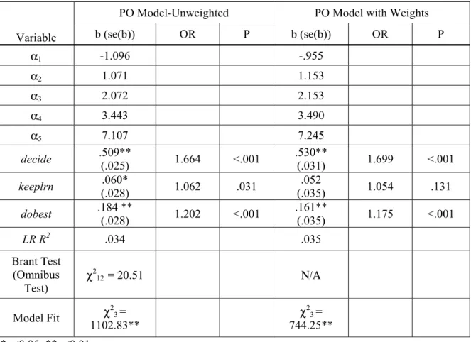
Table 4 presents a comparison of PO model results with and without weighted estimation. Compared to the unweighted PO model; all but the first cutpoints/intercepts slightly increased when sampling weights were specified in the PO model. Regarding the logit coefficients, the effect of one predictor (decide) increased and the other two, keeplrn and dobest, decreased. In addition, the standard errors of all three predictors increased. Specifically, when weights were applied to the PO model the estimated logit regression coefficient for getting no bad grades if deciding to (decide) increased by 4.1%, and its standard error increased by 24%, compared to those in the unweighted PO model; the logit coefficient for keeping studying if material is difficult (keeplrn) decreased by 15.4%, and its standard error increased by 25%; and the logit coefficient for doing best to learn (dobest) decreased by 14.3%, with its standard error increased by 25%.
In the unweighted PO model, the effects of all three predictors were significant. However, when weights were applied to the PO model, surprisingly only the first and last predictors were significant, and the second predictor (keeplrn) became insignificant, since the standard error was underestimated when weights were not applied.
Proportional Odds Model for Complex Survey Data Using Stata svy command
Finally, Stata’s survey data svy prefix command was used to fit the PO model, taking all the elements of survey design features, such as strata, cluster and weight variables into account. Before fitting the model, the svyset
command needed to be employed by specifying the complex sampling design variables and weights. In this example, the design features were specified as: svyset PSU [pweight = BYSTUWT], strata (STRAT_ID). In the svyset
command, the variable name for the primary sampling units or clusters in the data was PSU; the probability weight, pweight, was the student weight for the based year data (BYSTUWT), and the strata was START_ID. Figure 3 presents the result of the specified sampling design information.
242
Table 2: A Series (j-1=5) of Associated Binary Logistic Regression Models for the Full PO Model, where Each Split Compares Y > cat. j to Y≤ cat. j
Y > 0 Y > 1 Y > 2 Y > 3 Y > 4 Brant Test
P Value
Variable Logit (b) Logit (b) Logit (b) Logit (b) Logit (b)
Constant 1.413 -.989 -2.042 -3.639 -8.854
decide .502 .494 .507 .533 .910 .309
keeplrn -.017 .018 .060 .096 .296 .263
dobest .138 .208 .173 .187 .054 .607
Table 3: Brant Tests of the PO Assumption for Each Predictor and the Overall Model
Variable Test P Value
decide χ2 4 = 4.79 .309 keeplrn χ2 4 = 5.24 .263 dobest χ2 4 = 2.71 .607 All (Full-model) χ2 12 = 20.51 .058
Table 4: Comparison of the PO Models with and without Weighted Estimation
Variable
PO Model-Unweighted PO Model with Weights
b (se(b)) OR P b (se(b)) OR P α1 -1.096 -.955 α2 1.071 1.153 α3 2.072 2.153 α4 3.443 3.490 α5 7.107 7.245 decide .509** (.025) 1.664 <.001 .530** (.031) 1.699 <.001 keeplrn .060* (.028) 1.062 .031 .052 (.035) 1.054 .131 dobest .184 ** (.028) 1.202 <.001 .161** (.035) 1.175 <.001 LR R2 .034 .035 Brant Test (Omnibus Test) χ 2 12 = 20.51 Ν/Α Model Fit χ23 = 1102.83** χ 2 3 = 744.25** *p<0.05; **p<0.01
243
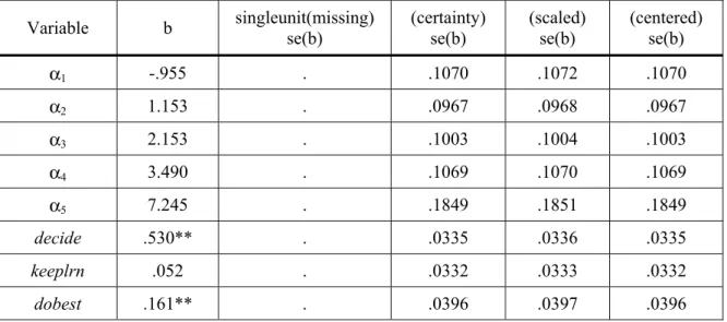
The result of the svyset output also indicated that by default missing values for the standard errors would be created when a stratum only contained a single sampling unit (single unit: missing). To deal with this singleton PSU issue, the svyset command provides the other three options (StataCorp, 2007), includingcertainty, scaled and centered. The first option,
singleunit(certainty) recognizes the single sampling unit in a stratum as a certainty unit (sampling unit chosen with 100% certainty), which contributes nothing to variance estimation across sampling units. The second option,
singleunit(scaled) is a scaled version of the first one, which uses the average variance of the strata with multiple PSUs for the stratum with a single sampling unit. The third option,
singleunit(centered) uses the grand mean across sampling units for variance estimation.
Each of these three options for the single unit was used separately in the svyset command because single sampling units resulted in missing standard errors in the model. Stata svy: ologit was then used to conduct for each survey ordinal logistic regression analysis. The results of the estimated standard errors using all singleunit options are shown in Table 5 and, because the singltunit(missing) is the default option, the missing values for standard error estimations are also provided.
The results of the standard errors estimated from all PO models were nearly the same. Therefore, only the result with the singleunit(certainty) option was reported in the following analysis. Figure 4 and Table 6 display the PO model result for complex survey data using svy: ologit.
Figure 3: Identifying the Sampling Design Variables and Weights Using the svyset Command . svyset PSU [pweight = BYSTUWT] , strata (STRAT_ID)
pweight: BYSTUWT VCE: linearized Single unit: missing Strata 1: STRAT_ID SU 1: PSU FPC 1: <zero>
Table 5: Estimated Standard Errors from the PO Models for Complex Survey Data with Four Singleunit() Options Variable b singleunit(missing) se(b) (certainty) se(b) (scaled) se(b) (centered) se(b) α1 -.955 . .1070 .1072 .1070 α2 1.153 . .0967 .0968 .0967 α3 2.153 . .1003 .1004 .1003 α4 3.490 . .1069 .1070 .1069 α5 7.245 . .1849 .1851 .1849 decide .530** . .0335 .0336 .0335 keeplrn .052 . .0332 .0333 .0332 dobest .161** . .0396 .0397 .0396
244
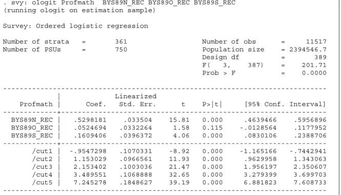
In the final PO model which accommodated sampling designs, Stata reports the the adjusted Wald test for all parameters rather than the log likelihood ratio Chi-Square test for the conventional PO model. F(3, 387) = 201.71, p < 0.001, suggested that the full model with three predictors was significant in predicting odds of being at or below a particular mathematics proficiency level.The logit effects of decide and dobest
were significant. For the predictor, decide, β = 0.530, t = 15.81, p < 0.001; and for the predictor,
dobest, β = 0.161, t = 4.06, p < 0.001. However, the effect of keeplrn was not significantly different from zero. β = 0.052, t = 1.58, p = 0.115.
Substituting the values of the estimated logit coefficients into the equation (3) resulted in logit [π(Y≤ j | X1, X2, X3)] = αj+ (−.530X1
−.052X2−.161X3). By exponentiating the
negative logit coefficients (e(-β)) the odds of
being at or below a particular proficiency level were obtained. Therefore, the odds of being at or below a particular proficiency level as opposed to being beyond that level for the three
predictors, decide, keeplrn, and dobest, were 0.589, 0.949 and 0.930, respectively.
When estimating the odds of being at or below a proficiency level, five cutpoints were used to differentiate adjacent categories of the mathematics proficiency. α1 = -0.955, which was
the cutpoint for the cumulative logit model for Y
≤ 0 (i.e., level 0 versus levels 1, 2, 3, 4, and 5); α2 was the cutpoint for the cumulative logit
model for Y ≤ 1 (i.e., levels 0 and 1 versus levels 2, 3, 4, and 5); and the final α5 was used
as the cutpoint for the logit model when Y ≤ 4. To estimate the odds of being beyond a proficiency level, equation (3) can be transformed to logit [π(Y > j | X1, X2, X3)] =
-αj+ .530X1 +.052X2 +.161X3. Odds ratios can be
calculated in the same way as above (see Table 6). In terms of odds ratio, getting no bad grades if deciding to (OR=1.699), and doing best to learn (OR = 1.175) was positively associated with the odds of being above a particular mathematics proficiency level, rather than being at or below that level. The OR for keeping learning when the material is difficult was 1.054, which was not significant.
Figure 4: PO Model for Complex Survey Data Using Stata svy: ologit
. svy: ologit Profmath BYS89N_REC BYS89O_REC BYS89S_REC (running ologit on estimation sample)
Survey: Ordered logistic regression
Number of strata = 361 Number of obs = 11517 Number of PSUs = 750 Population size = 2394546.7 Design df = 389 F( 3, 387) = 201.71 Prob > F = 0.0000 --- | Linearized
Profmath | Coef. Std. Err. t P>|t| [95% Conf. Interval] ---+--- BYS89N_REC | .5298181 .033504 15.81 0.000 .4639466 .5956896 BYS89O_REC | .0524694 .0332264 1.58 0.115 -.0128564 .1177952 BYS89S_REC | .1609406 .0396372 4.06 0.000 .0830106 .2388706 ---+--- /cut1 | -.9547298 .1070331 -8.92 0.000 -1.165166 -.7442941 /cut2 | 1.153029 .0966561 11.93 0.000 .9629958 1.343063 /cut3 | 2.153402 .1003036 21.47 0.000 1.956197 2.350607 /cut4 | 3.489551 .1068888 32.65 0.000 3.279399 3.699703 /cut5 | 7.245278 .1848627 39.19 0.000 6.881823 7.608733 --- Note: strata with single sampling unit treated as certainty units.
245
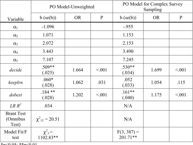
Comparison of Parameter and Standard Error Estimates from the PO model for Complex Survey Data and the Conventional Unweighted PO ModelTable 6 provides the parameter and standard error estimates obtained from the PO model for complex sampling data using Stata
svy: ologit and those from the unweighted PO model with Stata ologit. After sampling design variables and probability weights were applied to the PO model, the estimated logit coefficients and their standard errors were different from those in the unweighted PO model. The logit coefficient of the first predictor (decide) increased and those of the last two predictors (keeplrn and dobest) decreased. Further, the standard errors of all three coefficients increased tremendously.
Compared to the unweighted PO model, the estimated logit coefficient for getting no bad grades if deciding to (decide) in the PO model for complex survey data increased by 4.1%, and its standard error increased by 36%; the logit coefficient for keeping studying if material is difficult (keeplrn) decreased by 15.4%, and its standard error increased by 17.9%; and the logit coeffecit for doing best to learn (dobest) decreased by 14.3%, with its standard error increased by 42.9%.
The change of the parameter and linearized standard error estimates impacted significance tests. In the unweighted PO model, the effects of all three predictors were significant. However, when the sampling design variables and weights were applied to the PO model, only the first and last predictors were significant, and the second predictor (keeplrn) turned to be nonsignificant (p = 0.115).
Conclusion
This article explicated the use of the proportional odds models with complex survey sampling to estimate the ordinal response variable. Model fitting started from the conventional PO model without sampling weights, then the PO model with weights, and finally to the PO model for complex survey data with both weights and sampling design variables. Results of all three models were interpreted and compared. In addition, methods
of dealing with a single sampling unit within strata were illustrated and the estimated standard errors from the PO models with different single unit options were compared.
After sampling design variables and probability weights were applied to the conventional PO model, the estimated logit coefficients and their standard errors were more accurate than those in the unweighted PO model and the PO model with weights only. Specifically, first, compared to the unweighted PO model, the PO model with sampling weights impacts the accuracy of both parameter estimates and standard errors, and thus, the test statistics and the p-values; second, applying both the sampling weights and design variables to the PO model produced more accurate standard errors than the PO model with weights only, although these two models had the same parameter estimates.
This article demonstrated that ignoring weights, clusters and strata leads to biased parameter estimates and erroneous standard errors in ordinal logistic regression analysis. It extends the work by Hahs-Vaughn (2005, 2006), and Thomas and Heck (2001), which focused on the survey data analysis in multiple regression. Theories and mathematical details on how to estimate unbiased parameters and standard errors for complex survey data are well documented in literature and are beyond the scope of this article. Interested readers should refer to Binder (1983), Heeringa, West and Berglund (2010), Levy and Lemeshow (2008) and Lohr (1999) for details.
The logit coefficients in the PO model for complex survey data can be interpreted in the same way as those in the standard PO model. However, these two models may have different parameter estimates and standard errors, or even different levels of statistical significance (p-value). For example, the effect of one predictor in the above example became nonsignificant when weights and sampling design variables were applied to the conventional PO model.
In large-scale survey data, it is common to encounter a single sampling unit in a stratum, which results in the missing values of estimated standard errors in model fitting. This study suggests that any of the three single unit options, including certainty, scaled and centered, could
246
be used in the PO model to estimate standard errors.This article focused on the Taylor series approximation method for variance estimation. For future research, other variance estimation methods, such as the balanced repeated replication (BRR), the jackknife repeated replication (JRR) and the bootstrap method should be examined for ordinal logistic regression analysis. In addition, other general purpose statistical software packages, such as SPSS and SAS, may use different procedures or parameterizations in fitting PO models with complex survey data, which warrants further investigation. It is hoped that researchers will use the most appropriate models to analyze ordinal categorical dependent variables when data are collected using complex sampling designs.
Notes
Previous versions of this paper were presented at the Modern Modeling Methods Conference in Storrs, CT (May, 2012), the Northeastern Educational Research Association Annual Conference in Rocky Hill, CT (Oct., 2012), and 2013 Annual Meeting of American Educational Research Association (AERA), San Francisco, CA (April, 2013).
References
Agresti, A. (1996). An introduction to categorical data analysis. New York, NY: John Wiley & Sons.
Agresti, A. (2002). Categorical data analysis (2nd Ed.). New York, NY: John Wiley
& Sons.
Table 6: The PO Model Result for Complex Survey Data Using Stata svy:ologit Command (A Comparison with the Unweighted PO Model)
Variable
PO Model-Unweighted PO Model for Complex Survey Sampling
b (se(b)) OR P b (se(b)) OR P α1 -1.096 -.955 α2 1.071 1.153 α3 2.072 2.153 α4 3.443 3.490 α5 7.107 7.245 decide .509** (.025) 1.664 <.001 .530** (.034) 1.699 <.001 keeplrn (.028) .060* 1.062 .031 .052 (.033) 1.054 .115 dobest .184 ** (.028) 1.202 <.001 .161** (.040) 1.175 <.001 LR R2 .034 N/A Brant Test (Omnibus Test) χ 2 12 = 20.51 Ν/Α Model Fit/F test χ 2 3 = 1102.83** F(3, 387) = 201.71** *p<0.05; **p<0.01
247
Agresti, A. (2007). An introduction to categorical data analysis (2nd Ed.). New York, NY: John Wiley & Sons.Agresti, A. (2010). Analysis of ordinal categorical data (2nd Ed.). Hoboken, NJ: John
Wiley & Sons.
Allison, P.D. (1999). Logistic regression using the SAS system: Theory and application. Cary, NC: SAS Institute, Inc.
Ananth, C. V., & Kleinbaum, D. G. (1997). Regression models for ordinal responses: A review of methods and
applications. International Journal of
Epidemiology, 26, 1323-1333.
Armstrong, B. B., & Sloan, M. (1989). Ordinal regression models for epidemiological
data. American Journal of Epidemiology,
129(1), 191-204.
Binder, D. A. (1983). On the variances of asymptotically normal estimators from
complex surveys, International Statistical
Review,51, 279-292.
Brant (1990). Assessing proportionality in the proportional odds model for ordinal logistic regression. Biometrics, 46, 1171-1178.
Fienberg, S. E. (1980). The analysis of cross-classified categorical data. Cambridge, MA: The MIT Press.
Hardin, J. W., & Hilbe, J. M. (2007).
Generalized linear models and extensions (2nd Ed.). Texas: Stata Press.
Heeringa, S. G., West, B. T., & Berglund, P. A. (2010). Applied survey data analysis. Boca Raton, FL: Chapman & Hall/CRC.
Hahs-Vaughn, D. L. (2005). A primer for understanding and using weights with
national datasets. Journal of Experimental
Education, 73(3), 221-240.
Hahs-Vaughn, D. L., & Lomax, R. G. (2006). Utilization of sample weights in single level structural equation modeling. Journal of Experimental Education, 74(2), 163-190.
Hahs-Vaughn, D. L. (2006). Analysis of
data from complex samples. International
Journal of Research and Method in Education,
29(2), 163-181.
Hilbe, J. M. (2009). Logistic regression models. Boca Raton, FL: Chapman & Hall/CRC.
Hosmer, D. W., & Lemeshow, S. (2000). Applied logistic regression (2nd Ed.). New York, NY: John Wiley & Sons.
Ingels, S. J., Pratt, D. J., Roger, J., Siegel, P. H., & Stutts, E. (2004). ELS: 2002 Base Year Data File User’s Manual.
Washington, DC: NCES (NCES 2004-405). Ingels, S. J., Pratt, D. J., Roger, J., Siegel, P. H., & Stutts, E. (2005). Education Longitudinal Study: 2002/04 Public Use Base-Year to First Follow-up Data Files and Electronic Codebook System. Washington DC: NCES (NCES 2006-346).
Kalton, G. (1983). Introduction to
survey sampling. Beverly Hills, CA: Sage. Lee, E. S., & Forthofer, R. N. (2006).
Analyzing complex survey data (2nd Ed.).
Thousand Oaks, CA: Sage.
Levy, P. S., & Lemeshow, S. (2008).
Sampling of populations: Methods and application (4th Ed.). New York, NY: John
Wiley.
Liu, X. (2009). Ordinal regression analysis: Fitting the proportional odds model using Stata, SAS and SPSS. Journal of Modern Applied Statistical Methods, 8(2), 632-645.
Liu, X., O’Connell, A.A., & Koirala, H. (2011). Ordinal regression analysis: Predicting mathematics proficiency using the continuation
ratio model. Journal of Modern Applied
Statistical Methods, 10(2),513-527.
Liu, X., & Koirala, H. (2012). Ordinal regression analysis: Using generalized ordinal logistic regression models to estimate educational data. Journal of Modern Applied Statistical Methods, 11(1), 242-254.
Lohr, S. L. (1999). Sampling: Design and analysis. Pacific Grove, CA: Duxbury Press.
Long, J. S. (1997). Regression models for categorical and limited dependent variables. Thousand Oaks, CA: Sage.
Long, J. S. & Freese, J. (2006).
Regression models for categorical dependent variables using Stata (2nd Ed.). Texas: Stata
Press.
McCullagh, P. (1980). Regression models for ordinal data (with discussion).
Journal of the Royal Statistical Society Series B,
248
McCullagh, P. & Nelder, J. A. (1989).Generalized linear models (2nd Ed.). London: Chapman and Hall.
Menard, S. (1995). Applied logistic
regression analysis. Thousand Oaks, CA: Sage. Muthén, B. O., & Satorra, A. (1995). Complex sample data in structural equation modeling. Sociological Methodology, 25, 267-316.
O’Connell, A.A. (2000). Methods for modeling ordinal outcome variables.
Measurement and Evaluation in Counseling and Development, 33(3), 170-193.
O’Connell, A. A. (2006). Logistic
regression models for ordinal response variables. Thousand Oaks, CA: SAGE.
O’Connell, A. A., & McCoach, D. B. (2008). Multilevel modeling of educational data.
Charlotte, NC: IAP.
O’Connell, A.A., & Liu, X. (2011). Model diagnostics for proportional and partial proportional odds models. Journal of Modern Applied Statistical Methods, 10(1),139-175.
Powers D. A., & Xie, Y. (2000).
Statistical models for categorical data analysis. San Diego, CA: Academic Press.
Raudenbush, S. W., & Bryk, A. S.
(2002). Hierarchical linear models:
Applications and data analysis methods (2nd Ed.). Thousand Oaks, CA: Sage.
Stokes, M. E., Davis, C. S., & Koch, G. G. (2000). Categorical data analysis using the SAS system. Cary, NC: SAS Institute Inc.
Stapleton, L. M. (2002). The incorporation of sample weights into multilevel structural equation models. Structural Equation Modeling, 9(4), 475-502.
Stapleton, L. M. (2006). An assessment of practical solutions for structural equation modeling with complex sample data. Structural Equation Modeling, 13(1), 28-58.
Stapleton, L. M. (2008). Variance estimation using replication methods in structural equation modeling with complex sample data. Structural Equation Modeling,
15(2), 183-210.
StataCorp. (2007). Stata survey data reference manual. College Station, TX: Stata Press.
StataCorp. (2009). Stata survey data reference manual: Release 11. College Station, TX: Stata Press.
StataCorp. (2011). Stata survey data reference manual: Release 12. College Station, TX: Stata Press.
Thomas, S. L., & Heck, R. H. (2001). Analysis of large-scale secondary data in higher education research: Potential perils associated
with complex sampling designs. Research in