Reliability prediction based on complicated data and dynamic data

(1)

2009

Reliability prediction based on complicated data

and dynamic data

Yili Hong

Iowa State University

Follow this and additional works at:https://lib.dr.iastate.edu/etd Part of theStatistics and Probability Commons

This Dissertation is brought to you for free and open access by the Iowa State University Capstones, Theses and Dissertations at Iowa State University Digital Repository. It has been accepted for inclusion in Graduate Theses and Dissertations by an authorized administrator of Iowa State University Digital Repository. For more information, please [email protected].

Recommended Citation

Hong, Yili, "Reliability prediction based on complicated data and dynamic data" (2009).Graduate Theses and Dissertations. 10646.

(2)

by

Yili Hong

A dissertation submitted to the graduate faculty in partial fulfillment of the requirements for the degree of

DOCTOR OF PHILOSOPHY

Major: Statistics

Program of Study Committee: William Q. Meeker, Major Professor

Song Xi Chen Max D. Morris Sarah M. Ryan Huaiqing Wu

Iowa State University Ames, Iowa

2009

(3)

(4)

LIST OF TABLES

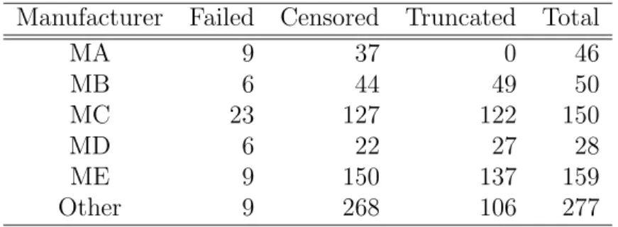
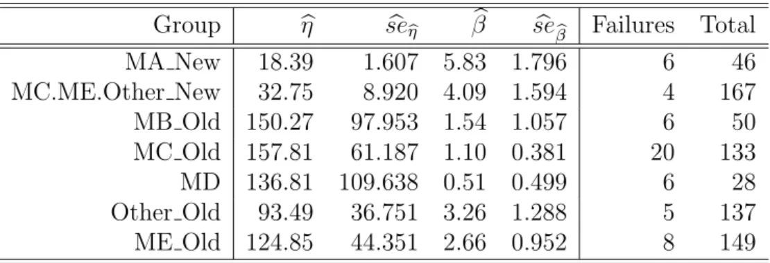
Table 2.1 Summary of the number of failed, censored, and truncated units for the different manufacturers. . . 17 Table 2.2 Weibull ML estimates of parameters and standard errors for each

group. . . 25 Table 2.3 Model comparison for the Old Group based on the Weibull

dis-tribution. . . 27 Table 2.4 Weibull ML estimates and confidence intervals for the Old group. 27 Table 2.5 Model comparison for the New Group based on the Weibull

dis-tribution. . . 28 Table 2.6 Weibull ML estimates and confidence intervals for the New Group. 29

Table 3.1 Values of the wrong-model parameters θ∗ for different censoring

times. . . 59 Table 3.2 ML estimates of the scale (η = exp(µ)) and shape (β = 1/σ)

pa-rameters of the Weibull distribution and 95% confidence intervals (CIs) based on the pooled-data and stratified-data models. . . . 68

Table 4.1 Summary of the Product D data . . . 81 Table 4.2 ML estimates and approximate confidence interval (CI) for

pa-rameters for the connected population. . . 86 Table 4.3 ML estimates and approximate CI for parameters for the

(10)

LIST OF FIGURES

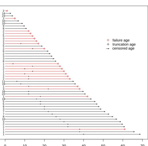
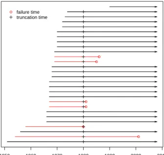
Figure 2.1 Service-time event plot of a systematic subset of the transformer lifetime data. The numbers in the left panel of the plot are counts for each line. . . 18 Figure 2.2 Weibull probability plot with the ML estimates of the cdfs for

each of the individual groups. . . 25 Figure 2.3 Weibull probability plots showing the ML estimates of the cdfs

for the Old group and the New group regression models. . . 28 Figure 2.4 Weibull distribution 90% prediction intervals for remaining life

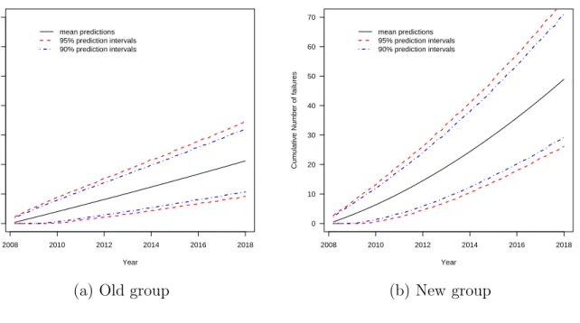
for a subset of individual at-risk transformers . . . 34 Figure 2.5 Weibull distribution predictions and prediction intervals for the

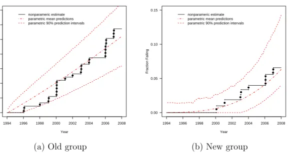
cumulative number of future failures. Number of units in risk set: Old 449, New 199. . . 37 Figure 2.6 Weibull distribution predictions and prediction intervals for the

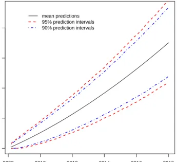
cumulative number of future failures with the Old and New groups combined. 648 units in risk set. . . 38 Figure 2.7 Weibull distribution predictions and prediction intervals for the

cumulative number of future failures for manufacturers MA and MB. Number of units in the risk set: MA 37, MB 44. . . 39 Figure 2.8 Sensitivity analysis for the effect that transformer lifetime

dis-tribution assumption has on the predicted cumulative number of future failures. . . 41

(11)

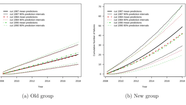
Figure 2.9 Sensitivity analysis for the effect that cutting year for the MC transformers has on the mean predicted number of failures. . . . 42 Figure 2.10 Back check of the model: parametric predictions compared with

Turnbull nonparametric estimates. . . 43 Figure 2.11 Calendar-time event plot for the MD group. . . 47 Figure 2.12 Contour plot of the Weibull distribution relative likelihood for

the MD Old group. . . 48

Figure 3.1 Comparison of hazard functions for the two sub-populations, the mixture of these two sub-populations, and the wrong model for three different values of the wrong-model parameters θ∗. . . 60

Figure 3.2 Comparison of the AMSE for the prediction based on the pooled-data and stratified-pooled-data models. . . 64 Figure 3.3 Event plot of the power transformer data. The numbers to the

right are the multiplicity of the corresponding events. . . 65 Figure 3.4 Weibull probability plot and the ML estimate based on

pooled-data model. . . 67 Figure 3.5 Weibull probability plot and the ML estimates based on the

stratified-data model. . . 67 Figure 3.6 Comparison of estimates of fraction failing extrapolated to 200

years, based on pooled-data and stratified-data models. . . 69 Figure 3.7 Comparison of the estimated AMSE for the prediction based on

the pooled-data and stratified-data models. . . 69

Figure 4.1 Histogram of use-rate for the connected units . . . 84 Figure 4.2 Lognormal probability plot for cycles-to-failure for all failure modes,

showing the corresponding ML estimates of the marginal cdfs for the connected population. . . 87

(12)

Figure 4.3 Lognormal probability plot of the system failure times along with the ML estimate of the series system failure time cdf. The ML estimates of the sub-distribution functions are also shown. . . 87 Figure 4.4 Lognormal probability plot for ML estimates for each failure

mode for the not-connected population. . . 90 Figure 4.5 shows the lognormal probability plot of the system failure times

along with the ML estimate of the series system failure time cdf. The ML estimates of the sub-distribution functions are also shown for the not-connected population. . . 91 Figure 4.6 (a) The predicted number of returns per week after the DFD due

to each failure mode for the connected population assuming the length of the warranty period is infinity.(b) Similar results but the warranty period is two years. . . 93 Figure 4.7 The predicted cumulative number of returns as a function of time

for each failure mode for the connected population and the 90% SPIs for the individual failure modes at certain time points. The vertical segments shows the SPIs for the individual failure modes. There are four segments at each time point. The x-location of these four SPIs are perturbed so that the lines will be visible. The small tick marks inside the plot at the bottom indicate the

x-locations of these SPIs. . . 94 Figure 4.8 The point predictions and pointwise PIs for the cumulative

num-ber of returns as a function of time after the DFD for the con-nected population. . . 96

(13)

Figure 4.9 The predicted cumulative number of returns as a function of time for each failure mode for the not-connected population and the 90% SPIs for the individual failure modes at certain time points. The vertical segments shows the SPIs for the individual failure modes. There are four segments at each time point. The x -location of these four SPIs are perturbed so that the lines will be visible. The small tick marks inside the plot at the bottom indicate thex-locations of these SPIs. . . 98 Figure 4.10 The point predictions and pointwise PIs for the cumulative

num-ber of returns as a function of time after the DFD for the not-connected population. . . 99 Figure 4.11 Comparison of prediction result for the failure-time data results

and cycles-to-failure data for the connected population. . . 101 Figure 4.12 Comparison of prediction result for the failure-time data results

and cycles-to-failure data for the not-connected population. . . 101 Figure 4.13 Comparisons of the asymptotic variance ratio for estimating

(14)

ACKNOWLEDGEMENTS

I would like to express my sincere gratitude to my major professor Dr. William Q. Meeker for his inspiring guidance, constructive suggestions and enthusiastic encourage-ment during my graduate study. I am also very grateful to my committee members, Drs. Songxi Chen, Max Morris, Sarah Ryan and Huaiqing Wu for their precious help. I am also very grateful to Dr. Luis A. Escobar from Department of Experimental Statistics, Louisiana State University, and Dr. James D. McCalley from Department of electri-cal and computer engineering, Iowa State University for the collaborations and help over these years. Graduate assistantships from Department of Statistics at Iowa State University and NSF Award CNS0540293 are acknowledged.

(15)

ABSTRACT

Lifetime data from the field can be complicated due to truncation, censoring, multi-ple failure modes, and the nonhomogeneity of the population. These complications lead to difficulties in reliability predictions and calibrations of the prediction intervals (PIs). Another trends in field lifetime data is the availability of the dynamic data which give in-formation dynamically on how a product being used and under which environment being used. Incorporating this information (historically not available) into statistical analyses will provide stronger statistical methods. In this dissertation, statistical models and methods motivated by real applications were developed for reliability predictions based on complicated data and dynamic data. In Chapter 2, left truncated and right censored high-voltage power transformer lifetime data are available from an energy company. The company wants to predict the remaining life of transformers and the cumulative number of failures at a future time for their transformer fleet. The population is nonhomoge-neous because transformer designs evolved over past decades. The data were stratified into relatively homogeneous groups and regression was done to incorporate the explana-tory variables. The random weighted bootstrap was used to overcome the difficulties introduced by the complicated structure of the data in the calibration of the prediction intervals. In Chapter 3, the importance of stratification when the population is nonho-mogeneous was analytically studied in the context of reliability predictions. There are two potential pitfalls for fitting a single distribution to nonhomogeneous data, which are misinterpretation of the failure mode and asymptotic biasness in prediction. These results were further illustrated by the high-voltage transformer life data. In Chapter 4,

(16)

data are available from a product which has four major failure modes. Use-rate infor-mation is available for units connected to the network. We use a cycles-to-failure model to compute predictions and prediction intervals for the number failing. We also present prediction methods for units not connected to the network.

(17)

CHAPTER 1. GENERAL INTRODUCTION

1.1 Background

Due to the expanding global marketplace and the resulting increased competition, today’s manufactures need to develop new, higher technology products while improving quality, reliability, and productivity. Manufacturers of high quality and high reliability products can have a strong competitive advantage in the market. As suggested by Condra (1993), reliability can be defined as “quality over time.” Achieving reliability requires careful focus on the time dimension. Statistical prediction of reliability of products based on reliability data is usually needed. These prediction can be used to detect product design deficiencies and to improve the product reliability of next product generation.

Because of the need of prediction, extrapolation is present in almost all applications. For example, we extrapolate in time when we have one year of data but have to pre-dict warranty returns going out three years. Parametric models, such as Weibull and lognormal, are often used for this purpose. The method of maximum likelihood and likelihood-based inference methods are used for the statistical inferences. In most appli-cations of reliability predictions, it is important to quantify statistical uncertainty (i.e., uncertainty due to limited data). Prediction intervals (PI) are the most commonly used method to do this. These PIs often need to be calibrated to provide the desired coverage probability (Meeker and Escobar 1998, Chapter 12, and Escobar and Meeker 1999).

(18)

1.1.1 Reliability Data Sources

Traditional reliability data have consisted of failure times for failed units and service times for surviving units. Laboratory life tests, field tracking studies, and warranty data bases are the three main sources of reliability data.

Accelerated life tests are often conducted to obtain information in a timely manner for a component must last for years or even decades. The basic idea is to test units at high levels of cycling rate, temperature, voltage, stress, or another accelerating variable to get reliability information quickly. Then a physically-motivated model is used to extrapolate to use conditions. See Nelson (2004) for more details on the statistical aspects of accelerated testing.

Although laboratory reliability testing is often used to make product design decisions, the “real” reliability data comes from the field, often in the form of warranty returns or, specially-designed field-tracking studies. Warranty databases provides a rich source of reliability information. Careful field tracking provides good reliability data. For example, good field data are often available for medical devices and a company’s fleet of assets.

1.1.2 Complexity of Field Data

Lifetime data from the field can be complicated due to multiple censoring, trun-cation, explanatory variables, multiple failure modes, and the non-homogeneity of the population, which lead to difficulties in reliability predictions and calibrations of pre-diction intervals (PIs). Komaki (1996) and Barndorff-Nielsen and Cox (1996) studied calibration of the naive “plug-in” PI procedure to account for statistical uncertainty using asymptotic expansions. Beran (1990), Meeker and Escobar (1998, Chapter 12), and Escobar and Meeker (1999) studied calibration of a naive PI using Monte Carlo simulation/bootstrap re-sampling methods for relatively simple situations. Lawless and

(19)

Fredette (2005) showed how to use a predictive distribution approach to provides PI that is the same as the calibrated naive PI. Statistical prediction procedures and the associated calibration needed to be developed for more complicated situations.

1.1.2.1 Censoring

Right-censored lifetime data result when unfailed units are still in service when data are analyzed. Multiple censoring resulted from staggered entry of units into the field. Methods for analyzing censored data (nonparametric estimation and maximum likeli-hood) have been well developed. See Meeker and Escobar (1998), and Lawless (2003) for more details for statistical methods for censored data.

1.1.2.2 Truncation

Truncation is different from censoring. Truncation arises when failure times are ob-served only when they take on values in a particular range. For observations that are outside the observation range, the existence of the unseen “observation” is not known. Thus, in some sense, the sample size is unknown! Ignoring truncation causes bias in es-timation. There are standard statistical methods for estimating distribution parameters with truncated data (i.e., data sampled from a truncated distribution(s)) described, for example, in Meeker and Escobar (2003), and Meeker and Escobar (1998, Chapter 11).

1.1.2.3 Explanatory variables

Explanatory variables can sometimes be used to explains why some units fail quickly and other units survive a long time. It is possible that estimates of quantities of interest could be biased seriously if important explanatory variables are ignored in an analysis. Incorporating explanatory variables can potentially explain more variabilities in field data. For details on parametric regression analysis for lifetime data, see, for example, Lawless (2003) or Meeker and Escobar (1998, Chapter 17).

(20)

1.1.2.4 Multiple failure modes

Products can fail due to different product failure modes. When the failure modes behave differently it is generally easier to find a well fitting failure-time distributions for the individual failure modes. In some applications, there is one failure mode that is of critical importance and others that are innocuous. Some failure modes are much more expensive to fix than others. This is important for forecasting warranty costs. When failure mode information is available for all failed units and when the different failure modes can be assumed to be statistically independent, the analysis of multiple failure mode data is, technically, not much more difficult than it is for analyzing a single failure mode. For single distribution applications in reliability, these methods are described and illustrated with examples in Nelson (1982, Chapter 5), and Meeker and Escobar (1998, Chapter 15). David and Moeschberger (1978), and Crowder (2001) are useful books on the subject of competing risks models and sub-distribution functions. These models are useful for modeling and predicting in reliability applications with multiple failure modes.

1.1.2.5 Population non-homogeneity

In field tracking studies, especially the studies that last a long time (e.g. several years or decades). The design of the product could evolve during the tracking period. Thus, the population is nonhomogeneous. A simple lifetime model fit to a pooled mixture of disparate populations can lead to incorrect conclusions. It is important to stratify all units into relatively homogeneous groups that have similar lifetime distributions.

1.1.3 The Next Generation of Reliability Data

Due to changes in technology, the next generation of reliability field data will be richer in information. Use rates and environmental conditions are important sources of variability in product lifetimes. The most important differences between carefully

(21)

controlled laboratory accelerated test experiments and field reliability results are due to uncontrolled field variation (unit-to-unit and temporal) in variables like use rate, load, vibration, temperature, humidity, UV intensity, and UV spectrum. Historically, use rate/environmental data has, in most applications, not been available to reliability ana-lysts. Incorporating use rate/environmental data into our analyses will provide stronger statistical methods.

Today it is possible to install sensors and smart chips in a product to measure and record use rate/environmental data over the life of the product. In addition to the time series use rate/environmental data, we also can expect to see further developments in sensors that will provide information, at the same rate, on degradation or indicators of eminent failure. Depending on the application, such information is also called “system health” and “materials state” information. In some applications (e.g., aircraft engines and power distribution transformers), system health/use rate/environmental data from a fleet of product in the field can be returned in real time to a central location for real-time process monitoring and especially for prognostic purposes. An appropriate signal in these data might provoke rapid action to avoid a serious system failure (e.g., by reducing the load on an unhealthy transformer). Also, should some issue relating to system health arise at a later date, it would be possible to use historical data that have been collected to see if there might have been a detectable signal that could be used in the future to provide an early warning of the problem.

In products that are attached to the internet (e.g., computers and high-end printers), such use rate/environmental data can, with the owner’s permission, be downloaded periodically. In some cases use/environmental data will be available on units only when they are returned for repair (although monitoring at least a sample of units to get information on unfailed units would be statistically important).

The future possibilities for using use rate/environmental data in reliability appli-cations are unbounded. Lifetime models that use rate/environmental data have the

(22)

potential to explain much more variability in field data than has been possible before. The information also can be used to predict the future environment lifetimes of individ-ual units. This knowledge can, in turn provide more precise estimates of the life time of individual products. As the cost of technology drops, cost-benefit ratios will decrease, and applications will spread.

1.2 Motivation

The main goal of purpose of this research is to develop prediction procedures that can be used to deal with data with a complicated structure and can use the dynamic information about the product use. This is research is motivated by real applications. The methodology that we developed, however, is general and can be applied to other situations. This section describes the motivation for the three projects in this disserta-tion.

1.2.1 Prediction for the Remaining Life of Power Transformers

Electrical transmission is an important part of the US energy industry. There are ap-proximately 150,000 high-voltage power transmission transformers in service in the US. Unexpected failures of transformers can cause large economic losses. Thus, prediction of remaining life of transformers is an important issue for the owners of these assets. The prediction of the remaining life can be based on historical lifetime information about the transformer population (or fleet). However, because the lifetimes of some transformers extend over several decades, transformer lifetime data are complicated.

In this project, we did the analysis of transformer lifetime data from an energy com-pany. Based on the currently available data, the company wants to know the remaining life of the healthy individual transformers in its fleet and the rate at which these trans-formers will fail over time. The energy company began careful archival record keeping

(23)

in 1980. The dataset provided to us contains complete information on all units that were installed after 1980 (i.e., the installation dates of all units and date of failure for those that failed). We also have information on units that were installed before January 1, 1980 and failed after January 1, 1980. We do not, however, have any information on units installed and failed before 1980. Thus, transformers that were installed before 1980 must be viewed as transformers sampled from truncated distribution(s). Units that are still in service have lifetimes that are right censored. Hence, the data are left truncated and right censored.

We present a statistical procedure for computing a prediction interval for remaining life for individuals and for the cumulative number failing in the future. We outline a general methodology for reliability prediction in complicated situations that involve the need for dealing with stratification, truncation, and censoring. In addition to describing our approach for dealing with these complications, we show how to produce calibrated prediction intervals by using the random weighted bootstrap and an approximation based on a refined central limit theorem.

1.2.2 The Importance of Stratification

It is well known that data from a mixture of two different distributions with in-creasing hazard functions can behave, over some period of time, like from a distribution with a decreasing hazard function (see Meeker and Escobar 1998, page 119 for a simple example). Thus, it is possible for predictions based on data from this kind of hetero-geneous population to lead to seriously incorrect conclusions. The lifetime distribution of a product is expected to have an increasing hazard function if the unit fails due to aging (wearout). For example, if a preliminary analysis of the pooled data indicates a decreasing or constant hazard function for what is known to be a wearout failure mode, it may be that one should stratify the data into relatively homogeneous subgroups and do prediction based on the stratified data.

(24)

This project was motivated by the reliability prediction problems described in Sec-tion 1.2.1. We simplified the setting by only considering the predicSec-tion of transformers manufactured by one manufacturer. The power transformer population consists of a mixture of two different designs, an old design and a new design. Both engineering knowledge and the data suggest that there is a difference between the old-design and the new-design transformers because the old transformers were often over-engineered. The life distribution estimate from the pooled data suggests a nearly constant hazard function, a result engineers who work with these transformers know to be wrong. How-ever, the estimates from stratified data suggest different increasing hazard functions for the different designs. Extrapolation to predict future failures from a constant hazard function model would, give incorrect answers.

We study the asymptotic properties of the maximum likelihood (ML) estimator under an incorrectly specified model to be used for prediction. We compare the asymptotic mean square error (AMSE) of predictions for the cumulative number of failing at a future time based both on the pooled-data model (inappropriate) and stratified-data model (appropriate). Results show that the prediction based on the pooled-data model can be seriously biased. We present an analysis of the power transformer data as an illustration.

1.2.3 Prediction Using Dynamic Use-Rate Information

In this project, we have data from a product what we will call Product D which is used in offices or residences. The use-rate (number of cycles of use per week where a cycle is a specific amount of product use, such as the typical amount of use in a day) information can be downloaded through a network if the unit is connected to the network. The use-rate information is not available for the units not connected to the network. Two specific problems arise in application. That is: “how to predict the number of warranty returns for the connected population using use-rate information?”

(25)

and “how to make similar predictions for the not-connected population using use-rate information from the connected population?”

The data were multiply censored due to staggered entry. We have cycles-to-failure information for all units that are connected to the network by taking a snapshot of the dynamic use-rate data at the data freeze date (DFD). Product D fails from causes that can be categorized into one of four major failure mode groups. In this project, we developed models and methods to incorporate the dynamic information. We used a cycles-to-failure model to compute predictions and prediction intervals for the number of returns. We also present prediction methods for units not-connected to the network. We showed that there are important advantages to using the cycles-to-failure data. That is, the prediction based on the cycles-to-failure data is more accurate and generally requires less extrapolation.

1.3 Dissertation Organization

This dissertation consists of three main chapters, preceded by the present general introduction and followed by a general conclusion. Each of these main chapter corre-sponds to a journal article. Chapter 2 presents the prediction of remaining life of power transformers and the prediction intervals based on left truncated and right censored life-time data. Chapter 3 studies the importance of identifying the components of a mixture in the context of prediction of field returns. Chapter 4 present the warranty prediction based on dynamic use-rate data.

(26)

Reference

Condra, L. W. (1993).Reliability Improvement with Design of Experiments. New York: Marcel Deeker.

Barndorff-Nielsen, O. and D. Cox (1996). Prediction and asymptotics. Bernoulli 2, 319–340.

Beran, R. (1990). Calibrating prediction regions.Journal of the American Statistical Association 85, 715–723.

Crowder, M. J. (2001). Classical Competing Risks. Boca Raton, FL: Chapman & Hall/CRC.

David, H. A. and M. L. Moeschberger (1978).The Theory of Competing Risks. London: Griffin.

Escobar, L. A. and W. Q. Meeker (1999). Statistical prediction based on censored life data. Technometrics 41, 113–124.

Komaki, F. (1996). On asymptotic properties of predictive distributions. Biometrika 83, 299–313.

Lawless, J. F. (2003). Statistical Models and Methods for Lifetime Data (2nd ed.). John Wiley and Sons Inc.

Lawless, J. F. and M. Fredette (2005). Frequentist prediction intervals and predictive distributions. Biometrika 92(3), 529–542.

(27)

Meeker, W. Q. and L. A. Escobar (1998).Statistical Methods for Reliability Data. New York: John Wiley & Sons, Inc.

Meeker, W. Q. and L. A. Escobar (2003). Use of Truncated Regression Methods to Estimate the Shelf Life of a Product from Incomplete Historical Data, Chapter 12. Case Studies in Reliability and Maintenance. John Wiley & Sons: New York.

Nelson W. (1982).Applied Life Data Analysis. New York: John Wiley & Sons, Inc.

Nelson W. (2004).Accelerated Testing: Statistical Models, Test Plans, and Data Anal-yses. New York: John Wiley & Sons, Inc (updated paperback version of the original 1990 book).

(28)

CHAPTER 2. PREDICTION OF REMAINING LIFE OF

POWER TRANSFORMERS BASED ON LEFT

TRUNCATED AND RIGHT CENSORED LIFETIME DATA

A paper published in the Annals of Applied Statistics

Yili Hong and William Q. Meeker Department of Statistics

Iowa State University Ames, IA, 50011, USA

James D. McCalley

Department of Electrical and Computer Engineering Iowa State University

Ames, IA, 50011, USA

Abstract

Prediction of the remaining life of high-voltage power transformers is an important issue for energy companies because of the need for planning maintenance and capital expendi-tures. Lifetime data for such transformers are complicated because transformer lifetimes can extend over many decades and transformer designs and manufacturing practices have evolved. We were asked to develop statistically-based predictions for the lifetimes of an

(29)

energy company’s fleet of high-voltage transmission and distribution transformers. The company’s data records begin in 1980, providing information on installation and failure dates of transformers. Although the dataset contains many units that were installed before 1980, there is no information about units that were installed and failed before 1980. Thus, the data are left truncated and right censored. We use a parametric lifetime model to describe the lifetime distribution of individual transformers. We develop a sta-tistical procedure, based on age-adjusted life distributions, for computing a prediction interval for remaining life for individual transformers now in service. We then extend these ideas to provide predictions and prediction intervals for the cumulative number of failures, over a range of time, for the overall fleet of transformers.

Key Words: Maximum likelihood; random weighted bootstrap; reliability; regres-sion analysis; transformer maintenance.

2.1 Introduction

2.1.1 Background

Electrical transmission is an important part of the US energy industry. There are ap-proximately 150,000 high-voltage power transmission transformers in service in the US. Unexpected failures of transformers can cause large economic losses. Thus, prediction of remaining life of transformers is an important issue for the owners of these assets. The prediction of the remaining life can be based on historical lifetime information about the transformer population (or fleet). However, because the lifetimes of some transformers extend over several decades, transformer lifetime data are complicated.

This paper describes the analysis of transformer lifetime data from an energy com-pany. Based on the currently available data, the company wants to know the remaining life of the healthy individual transformers in its fleet and the rate at which these trans-formers will fail over time. To protect sensitive and proprietary information, we will not

(30)

use the name of the company. We also code the name of the transformer manufacturers and modify the serial numbers of the transformers in the data. We use a parametric life-time model to describe the lifelife-time distribution of individual transformers. We present a statistical procedure for computing a prediction interval for remaining life for individuals and for the cumulative number failing in the future.

The energy company began careful archival record keeping in 1980. The dataset provided to us contains complete information on all units that were installed after 1980 (i.e., the installation dates of all units and date of failure for those that failed). We also have information on units that were installed before January 1, 1980 and failed afterJanuary 1, 1980. We do not, however, have any information on units installed and failed before 1980. Thus, transformers that were installed before 1980 must be viewed as transformers sampled from truncated distribution(s). Units that are still in service have lifetimes that are right censored. Hence, the data are left truncated and right censored. For those units that are left truncated or right censored (or both), the truncation times and censoring times differ from unit-to-unit because of the staggered entry of the units into service.

There are standard statistical methods for estimating distribution parameters with truncated data described, for example, in Meeker and Escobar (2003), and Meeker and Escobar (1998, Chapter 11) but such methods appear not to be available in commercial software. Meeker and Escobar (2008), a free package for reliability data analysis, does allow for truncated data. Most of the computations needed to complete this paper, however,required extending this software.

In this paper, we outline a general methodology for reliability prediction in compli-cated situations that involve the need for dealing with stratification, truncation, and censoring. In addition to describing our approach for dealing with these complications, we show how to produce calibrated prediction intervals by using the random weighted bootstrap and an approximation based on a refined central limit theorem.

(31)

2.1.2 A General Approach to Statistical Prediction of Transformer Life

Our approach to the prediction problem will be divided into the following steps. 1.Stratification: A simple lifetime model fit to a pooled mixture of disparate pop-ulations can lead to incorrect conclusions. For example, engineering knowledge suggests that there is an important difference between old transformers and new transformers because old transformers were over-engineered. Thus, we first stratify all transform-ers into relatively homogeneous groups that have similar lifetime distributions. This grouping will be based on manufacturer and date of installation. The groupings will be determined from a combination of knowledge of transformer failure mechanisms, man-ufacturing history, and data analysis. Each group will have its own set of parameters. The parameters will be estimated from the available lifetime data by using the maximum likelihood (ML) method. We may, however, be able to reduce the number of parameters needed to be estimated by, for example, assuming a common shape parameter across some of the groups (from physics of failure, we know that similar failure modes can often be expected to be described by distributions with similar shape parameters).

2. Lifetime Distribution: Estimate the lifetime probability distribution for each group of transformers from the available lifetime data.

3. Remaining Life Distribution: Identify all transformers that are at risk to fail (the “risk set”). Each of these transformers belongs to one of the above-mentioned groups of transformers. For each transformer in the risk set, compute an estimate of the distribution of remaining life (this is the conditional distribution of remaining life, given the age of the individual transformer).

4. Expected Number of Transformers Failing: Having the distribution of re-maining life on each transformer that is at risk allows the computation of the estimated expected number of transformers failing in each future interval of time (e.g., future months). We use this estimated expected number failing as a prediction of population

(32)

behavior.

5. Prediction Intervals: It is also important to compute prediction intervals to account for the statistical uncertainty in the predictions (statistical uncertainty accounts for the uncertainty due to the limited sample size and the variability in future failures, but assumes that the statistical model describing transformer life is correct).

6.Sensitivity Analysis: To compute our predictions we need to make assumptions about the stratification and lifetime distributions. There is not enough information in the data or from the engineers at the company to be certain that these assumptions are correct. Thus, it is important to perturb the assumptions to assess their effect on answers.

2.1.3 Overview

The rest of the paper is organized as follows. Section 2.2 describes our exploratory analysis of the transformer lifetime data and several potentially important explanatory variables. Section 2.3 describes the model and methods for estimating the transformer lifetime distributions. Section 2.4 gives details on stratifying the data into relatively homogeneous groups and our regression analyses. Section 2.5 shows how estimates of the transformer lifetime distributions lead to age-adjusted distributions of remaining life for individual transformers and how these distributions can be used as a basis for com-puting a prediction interval for remaining life for individual transformers. Section 2.6 provides predictions for the cumulative number of failures for the overall population of transformers now in service, as a function of time. Section 2.7 presents sensitivity anal-ysis on the prediction results. Section 2.8 concludes with some discussion and describes areas for future research.

(33)

Table 2.1 Summary of the number of failed, censored, and truncated units for the different manufacturers.

Manufacturer Failed Censored Truncated Total

MA 9 37 0 46 MB 6 44 49 50 MC 23 127 122 150 MD 6 22 27 28 ME 9 150 137 159 Other 9 268 106 277

2.2 The Transformer Lifetime Data

The dataset used in our study contains 710 observations with 62 failures. Table 2.1 gives a summary of the number of failed, censored, and truncated units for the different manufacturers. Figure 3.3 is an event plot of a systematic subset of the data.

2.2.1 Failure Mechanism

Transformers, for the most part, fail when voltage stress exceeds the dielectric strength of the insulation. The insulation in a transformer is made of a special kind of paper. Over time, the paper will chemically degrade, leading to a loss in dielectric strength, and eventual failure. The rate of degradation depends primarily on operating temperature. Thus, all other things being equal, transformers that tend to run at higher load, with correspondingly higher temperatures, would be expected to fail sooner than those running at lower loads. Events such as short circuits on the transmission grid can cause momentary thermal spikes that can be especially damaging to the insulation.

2.2.2 Early Failures

Seven units failed within the first 5 years of installation. The lifetimes for these units are short compared with the vast majority of units that failed or will fail with age

(34)

Years of Service 0 10 20 30 40 50 60 70 1 1 1 1 2 3 108 7 7 3 9 5 5 191 22 163 1 16 112 2 1 1 2 1 1 8 3 3 2 6 2 5 3 2 3 5 2 2 8 9 10 102 23 142 failure age truncation age censored age

Figure 2.1 Service-time event plot of a systematic subset of the transformer lifetime data. The numbers in the left panel of the plot are counts for each line.

(35)

greater than 10 years. These early failures are believed to have been due to a defect related failure mode that is different from all of the other failures. The inclusion of these early failures in the analysis leads to an indication of an approximately constant hazard function for transformer life, which is inconsistent with the known predominant aging failure mode. Thus, we considered these early failures to be right censored at the time of failure. This is justified because the primary goal of our analysis is to model the failure mode for the future failures for the remaining units. It is reasonable to assume that there are no more defective units in the population for which predictions are to be generated.

2.2.3 Explanatory Variables

Engineering knowledge suggests that the insulation type and cooling classes may have an effect on the lifetime of transformers. Thus, the effects that these two variables have on lifetime are studied in this paper.

2.2.3.1 Insulation

The transformers are rated at either 55 or 65 degree rise. This variable defines the average temperature rise of the winding, above ambient, at which the transformer can operate in continuous service. For example, a 55 degree-rise rated transformer operated at a winding temperature of 95 degrees should, if the engineering model describing this phenomena is adequate, have the same life as a 65 degree-rise rated transformer operated at a winding temperature of 105 degrees. The two categories of the insulation class are denoted by “d55” and “d65”, respectively.

2.2.3.2 Cooling

A transformer’s cooling system consists of internal and external subsystems. The internal subsystem uses either natural or forced flow of oil. Forced flow is more efficient.

(36)

The external cooling system uses either air or water cooling. Water cooling is more efficient. The external cooling media circulation is again either natural or forced. Forced circulation is usually used on larger units and is more efficient but is activated only when temperature is above a certain threshold. The cooling methods for the transformers in the data are categorized into four groups: natural internal oil and natural external air/water (NINE), natural internal oil and forced external air/water (NIFE), forced internal oil and forced external air/water (FIFE), and unknown.

2.3 Statistical Lifetime Model for Left Truncated and Right

Censored Data

2.3.1 The Lifetime Model

We denote the lifetime of a transformer byT and model this time with a log-location-scale distribution. The most commonly used distributions for lifetime, the Weibull and lognormal, are members of this family. The cumulative distribution function (cdf) of a log-location-scale distributions can be expressed as

F(t;µ, σ) = Φ

log(t)₋µ σ

where Φ is the standard cdf for the location-scale family of distributions (location 0 and scale 1), µ is the location parameter, and σ is the scale parameter. The corresponding probability density function (pdf) is the first derivative of the cdf with respect to time and is given by f(t;µ, σ) = 1 σtφ log(t)₋µ σ

where φ is the standard pdf for the location-scale family of distributions. The hazard function ish(t;µ, σ) =f(t;µ, σ)/[1₋F(t;µ, σ)]. For the lognormal distribution, replace Φ and φ above with Φnor and φnor, the standard normal cdf and pdf, respectively. The

(37)

cdf and pdf of the Weibull random variable T are F(t;µ, σ) = Φsev log(t)₋µ σ and f(t;µ, σ) = 1 σtφsev log(t)₋µ σ

where Φsev(z) = 1−exp[−exp(z)] and φsev(z) = exp[z −exp(z)] are the standard (i.e., µ= 0, σ = 1) smallest extreme value cdf and pdf, respectively. The cdf and pdf of the Weibull random variable T can also be expressed as

F(t;η, β) = 1₋exp " − t η β# and f(t;η, β) = β η t η β−1 exp " − t η β#

where η = exp(µ) is the scale parameter and β = 1/σ is the shape parameter. If the Weibull shape parameterβ >1, the Weibull hazard function is increasing (corresponding to wearout); if β = 1, the hazard function is a constant; and if β < 1, the hazard function is decreasing. The location-scale parametrization is, however, more convenient for regression analysis.

2.3.2 Censoring and Truncation

Right-censored lifetime data result when unfailed units are still in service (unfailed) when data are analyzed. A transformer still in service in March 2008 (the “data-freeze” point) is considered as a censored unit in this study.

Truncation, which is similar to but different from censoring, arises when failure times are observed only when they take on values in a particular range. When the existence of the unseen “observation” is not known for observations that fall outside the particular range, the data that are observed are said to be truncated. Because we have no informa-tion about transformers that were installed and failed before 1980, the units that were installed before 1980 and failed after 1980 should be modeled as having been sampled from a left-truncated distribution. Ignoring truncation causes bias in estimation.

(38)

2.3.3 Maximum Likelihood Estimation

Let ti denote the lifetime or survival time of transformer i, giving the number of

years of service between the time the transformer was installed until it failed (for a failed transformer) or until the data-freeze point (for a surviving transformer). Here,

i = 1,_{· · ·}, n, where n is the number of transformers in the dataset. Let τL

i be the

left truncation time, giving the time at which the life distribution of transformer i was truncated on the left. More precisely,τL

i is the number of years between the transformer’s

manufacturing date and 1980 for transformers installed before 1980. Let νi be the

truncation indicator. In particular, νi = 0 if transformer i is truncated (installed before

1980) and νi = 1 if transformer i is not truncated (installed after 1980). Let ci be

the censoring time (time that a transformer has survived) and let δi be the censoring

indicator. In particular, δi = 1 if transformer i failed andδi = 0 if it was censored (not

yet failed).

The likelihood function for the transformer lifetime data is

L(θ_|DAT A) = n Y i=1 f(ti;θ)δiνi× f(ti;θ) 1₋F(τL i ;θ) δi(1−νi) (2.1) ×[1₋F(ci;θ)](1−δi)νi× 1₋F(ci;θ) 1₋F(τL i ;θ) (1−δi)(1−νi) .

Here θ is a vector that gives the location parameter (µi) and scale parameters (σi) for

each transformer. The exact structure of θ depends on the context of the model. For example, in Section 2.4.1, we stratify the data into J groups with nj transformers in

group j and fit a single distribution to each group. For this model we assume that observations from group j have the same location (µj) and scale parameters (σj). Thus,

θ = (µ1,· · · , µ1 | {z } Group 1 ,_{· · ·} , µJ,· · · , µJ | {z } GroupJ , σ1,· · · , σ1 | {z } Group 1 ,_{· · ·}, σJ,· · · , σJ | {z } GroupJ )′_.

For notational simplicity, we also use F(ti;θ) = F(ti;µi, σi) and f(ti;θ) = f(ti;µi, σi).

(39)

ML estimate bθ is obtained by finding the values of the parameters that maximize the likelihood function in (2.1).

2.4 Stratification and Regression Analysis

2.4.1 Stratification

As described in Section 2.1.2, we need to stratify the data into relatively homoge-neous groups. Manufacturer and installation year were used as preliminary stratification variables. The choice of installation year as the stratification variable is strongly moti-vated by the design change of transformers. There is a big difference between the old transformers and new transformers. The engineers indicate that old transformers were over-engineered and can last a long time. For example, there are transformers installed in 1930s that are still in service, as shown in Figure 3.3. Due to the competition in the transformer manufacture industry and the need of reducing manufacturing costs, the new transformers are not as “strong” as old ones.

The transformers manufactured by the same manufacturer were divided into two groups (New and Old) based on age (installation year). We chose the cutting year for this partitioning to be 1987. In Section 2.7.1, we give the results of a sensitivity analysis that investigated the effects of changing the cutting year. There are only one or two failures in some groups (i.e., MC New, ME New, and Other New). These groups were combined together as MC.ME.Other New. Note that all MA units were installed after 1990 and all MB units were installed before 1987.

Figure 2.2 is a multiple Weibull probability plot showing the nonparametric and the Weibull ML estimates of the cdf for all of the individual groups. The nonparametric estimates (those points in Figure 2.2) are based on the method for truncated/censored data described in Turnbull (1976). The points in Figure 2.2 were plotted at each observed lifetime (censored units were not plotted) and at the midpoint of the step of the Turnbull

(40)

cdf estimates, as suggested in Meeker and Escobar (1998, Section 6.4.2) and Lawless (2003, Section 3.3). Table 2.2 gives the ML estimates and standard errors of the Weibull distribution parameters for each group.

Note that the nonparametric and the parametric estimates in Figure 2.2 do not agree well for the Old groups. This is due to the truncation in these groups. When sampling from a truncated distribution, the ML estimator based on the likelihood in (2.1) is consistent. The nonparametric estimator used in the probability plots, however, is not consistent if all observations are truncated. Because almost all of the observations are truncated in the Old groups, we would not expect the parametric and nonparametric estimates to agree well, even in moderately large finite samples.

Based on the ML estimates for the individual groups, the dataset was partitioned into two large groups: the Old group with slowly increasing hazard rate (βb_≈2), and the New group with a more rapidly increasing hazard rate (βb_≈5). The Old group consists of MB Old, MC Old, Other Old and ME Old, and the New group consists of MA New and MC.ME.Other New. When we do regression analyses in Section 2.4.4, we assume that there is a common shape parameter for all of the transformers in theOld groupand a different common shape parameter for all of the transformers in the New group. This assumption is supported by the lifetime data as can be seen in Figure 2.2 and by doing likelihood ratio tests (details not given here).

2.4.2 Distribution Choice

We also fit individual lognormal distributions and made a lognormal probability plot (not shown here) that is similar to Figure 2.2. Generally, the Weibull distributions fit somewhat better, both visually in the probability plot and in terms of the loglikelihood values of the ML estimates. There is a physical/probabilistic explanation for this con-clusion. In the transformer, there are many potential locations where the voltage stress could exceed the dielectric stress. The transformer will fail the first time such an event

(41)

Years .001 .003 .005 .01 .02 .03 .05 .1 .2 .3 .5 .7 .9 5 10 20 50 100 200 Fraction Failing MA_New MB_Old MC.ME.Other_New MC_Old MD_Old Other_Old ME_Old

Figure 2.2 Weibull probability plot with the ML estimates of the cdfs for each of the individual groups.

Table 2.2 Weibull ML estimates of parameters and standard errors for each group.

Group η_b se_bη_b βb sebβb Failures Total

MA New 18.39 1.607 5.83 1.796 6 46 MC.ME.Other New 32.75 8.920 4.09 1.594 4 167 MB Old 150.27 97.953 1.54 1.057 6 50 MC Old 157.81 61.187 1.10 0.381 20 133 MD 136.81 109.638 0.51 0.499 6 28 Other Old 93.49 36.751 3.26 1.288 5 137 ME Old 124.85 44.351 2.66 0.952 8 149

(42)

occurs. That is, a transformer’s lifetime is controlled by the distribution of a minimum. The Weibull distribution is one of the limiting distribution of minima.

2.4.3 A Problem with the MD Group Data

As shown in Table 2.2, the estimate of the Weibull shape parameter for the MD group is βb= 0.51, implying a strongly decreasing hazard function. Such a decreasing hazard is not consistent with the known aging failure mode of the transformer insulation. This problem with the estimation is caused by the extremely heavy truncation. More details about this estimation problem are available in the supplemental materials of this paper. As a remedy, in the estimation and modeling stage, we exclude the MD units. When we make the predictions, however, we include the MD Old units that are currently in service in the Old group and the single MD New unit in the New group based on engineering knowledge about the designs.

2.4.4 Regression Analysis

In this section, we extend the single distribution models fit in Section 2.4.1 to re-gression models. For details on parametric rere-gression analysis for lifetime data, see, for example, Lawless (2003) or Meeker and Escobar (1998, Chapter 17). In our models, the location parameter µis treated as a function of explanatory variable x, denoted by

µ(x) = g(x,β) where x = (x1, x2,· · · , xp)′ and β = (β0, β1,· · · , βp)′. In the case of

linear regression g(x,β) =x′β.

We fit separate regression models for the strata identified in Section 2.4.1 in the next two sections. The explanatory variables considered in the regression modeling are

(43)

Table 2.3 Model comparison for the Old Group based on the Weibull dis-tribution.

Model loglikelihood

1 µ(x) = Cooling -103.663

2 µ(x) = Manufacturer + Cooling -100.268

3 µ(x) = Manufacturer+Cooling+Insulation -100.198

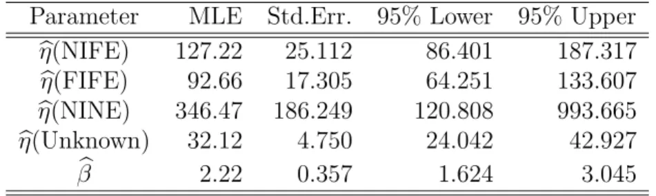
Table 2.4 Weibull ML estimates and confidence intervals for the Old group.

Parameter MLE Std.Err. 95% Lower 95% Upper b η(NIFE) 127.22 25.112 86.401 187.317 b η(FIFE) 92.66 17.305 64.251 133.607 b η(NINE) 346.47 186.249 120.808 993.665 b η(Unknown) 32.12 4.750 24.042 42.927 b β 2.22 0.357 1.624 3.045

2.4.4.1 The Old group

Table 2.3 compares the loglikelihood values for the Weibull regression models fit to the Old group. Likelihood ratio tests show that Manufacturer and Insulation are not statistically important (i.e., the values of the loglikelihood for Models 2 and 3 are only slightly larger then that for Model 1). Hence, the final model for the Old group is

µ(x)=Cooling. Table 2.4 gives ML estimates and confidence intervals for parameters for the final model for the Old group. Figure 2.3a gives the Weibull probability plot showing the Weibull regression estimate of the cdfs for the different cooling categories. The slopes of the fitted lines are the same because of the constant shape parameter assumption in our model.

(44)

Years .001 .003 .005 .01 .02 .03 .05 .1 .2 .3 .5 .7 .9 5 10 20 50 100 200 Fraction Failing NIFE FIFE NINE Unknown Years .001 .003 .005 .01 .02 .03 .05 .1 .2 .3 .5 .7 .9 5 10 20 50 100 200 Fraction Failing MA_New MC.ME.Other_New

(a) Old group (b) New group

Figure 2.3 Weibull probability plots showing the ML estimates of the cdfs for the Old group and the New group regression models.

Table 2.5 Model comparison for the New Group based on the Weibull dis-tribution.

Model loglikelihood

4 µ(x) = µ -25.268

5 µ(x) = Manufacturer -20.138

6 µ(x) = Manufacturer + Cooling -18.089

2.4.4.2 The New group

Table 2.5 compares the loglikelihood values for the Weibull regression models fit to the New group. Insulation is not in the model because it only has one level in the

New group. Likelihood ratio tests show that Manufacturer is statistically important. Hence, the final model for the New group is µ(x) =Manufacturer. Table 2.6 gives ML estimates and confidence intervals for the final regression model parameters for the New group. Figure 2.3b is a Weibull probability plot showing the ML estimates of the cdfs for the two manufacturers in this group.

(45)

Table 2.6 Weibull ML estimates and confidence intervals for the New Group.

Parameter MLE Std.Err. 95% Lower 95% Upper b η(MA New) 18.94 1.850 15.641 22.936 b η(MC.ME.Other New) 29.29 4.548 21.602 39.706 b β 5.01 1.229 3.098 8.104

2.5 Predictions for the Remaining Life of Individual

Transformers

In this section, we develop a prediction interval procedure to capture, with 100(1₋

α)% confidence, the future failure time of an individual transformer, conditional on survival until its present age,ti. The prediction interval is denoted by

h

T

ei, Tei i

.The

cdf for the lifetime of a transformer, conditional on surviving until time ti, is

F(t_|ti;θ) = Pr(T ≤t|T > ti) =

F(t;θ)₋F(ti;θ)

1₋F(ti;θ)

, t_≥ti. (2.2)

This conditional cdf provides the basis of our predictions and prediction intervals.

2.5.1 The Naive Prediction Interval Procedure

A simple naive prediction interval procedure (also known as the “plug-in” method) provides an approximate interval that we use as a start toward obtaining a more refined interval. The procedure simply takes the ML estimates of the parameters and substitutes them into the estimated conditional probability distributions in (2.2) (one distribution for each transformer). The estimated probability distributions can then be used as a basis for computing predictions and prediction intervals. Let 100(1 ₋α)% be the nominal coverage probability. The coverage probability is defined as the probability that the prediction interval procedure will produce an interval that captures what it is intended to capture.

(46)

The naive 100(1₋α)% prediction interval for a transformer having agetiis h T ei, Tei i whereT

eiandTeisatisfyF(Tei|ti,bθ) =αl, F(Tei|ti,bθ) = 1−αu.Hereαlandαuare the lower and upper tail probabilities, respectively and αl+αu =α. We choose αl = αu = α/2.

This simple procedure ignores the uncertainty in bθ. Thus, the interval coverage prob-ability of this simple procedure is generally smaller than the nominal confidence level. The procedure needs to be calibrated so that it will have a coverage probability that is closer to the nominal confidence level.

2.5.2 Calibration of the Naive Prediction Interval

Calibration of the naive prediction interval procedure to account for statistical un-certainty can be done through asymptotic expansions (Komaki 1996, Barndorff-Nielsen and Cox 1996) or by using Monte Carlo simulation/bootstrap re-sampling methods (Be-ran 1990 and Escobar and Meeker 1999). Lawless and Fredette (2005) show how to use a predictive distribution approach that provides intervals that are the same as the calibrated naive prediction interval.

In practice, simulation is much easier and is more commonly used to calibrate naive prediction interval procedures. In either case, the basic idea is to find an input value for the coverage probability (usually larger than the nominal value) that gives a proce-dure that has the desired nominal coverage probability. In general the actual coverage probability of a procedure employing calibration is still only approximately equal to the nominal confidence level. The calibrated procedure, if it is not exact (i.e. actual cov-erage probability is equal to the nominal), can be expected to provide a much better approximation than the naive procedure.

(47)

2.5.3 The Random Weighted Bootstrap

Discussion of traditional bootstrap resampling methods for lifetime/survival data can be found, for example, in Davison and Hinkley (1997). Due to the complicated data structure and sparsity of failures over the combinations of different levels of explana-tory variables, however, the traditional bootstrap method is not easy to implement and may not perform well. Bootstrapping with the commonly used simple random sampling with replacement with heavy censoring can be problematic as it can result in bootstrap samples without enough failures for the estimation of parameters (only about 9% of the transformers had failed). A parametric bootstrap would require distribution assump-tions on the truncation time and censoring time and this information is not available. The stratification, regression modeling, and especially the left truncation, lead to other difficulties with bootstrapping. The random weighted likelihood bootstrap procedure, introduced by Newton and Raftery (1994), provides a versatile, effective, and easy-to-use method to generate bootstrap samples for such more complicated problems. The procedure uses the following steps:

1. Simulate random valuesZi, i= 1,2,· · · , nthat arei.i.d. from a distribution having

the property E(Zi) = [Var(Zi)]1/2.

2. The random weighted likelihood is L∗₍_θ

|DAT A) = Qn_i₌₁[Li(θ|DAT A)]Zi where

Li(θ|DAT A) is the likelihood contribution from an individual observation.

3. Obtain the ML estimate bθ∗ by maximizing L∗₍_θ

|DAT A).

4. Repeat step 1-3 B times, to getB bootstrap samples bθ∗_b, b= 1,2,_{· · ·} , B.

Barbe and Bertail (1995, Chapter 2) discuss how to choose the random weights by using an Edgeworth expansion. Jin, Ying, and Wei (2001) showed that the distribution of √_n₍_θ_b∗

(48)

√

n(θb₋θ), if one uses i.i.d. positive random weights generated from continuous dis-tribution with E(Zi) = [Var(Zi)]1/2. They pointed out that the resampling method is

rather robust for different choices of the distribution of Zi, under this condition. We

used Zi ∼ Gamma(1,1) in this paper. We also tried alternative distributions, such as

the Gamma(1,0.5), Gamma(1,2), and Beta(√2₋1,1). The resulting intervals were insensitive to the distribution used, showing similar robustness for our particular appli-cation.

2.5.4 Calibrated Prediction Intervals

For an individual transformer with age ti, the calibrated prediction interval of

re-maining life can be obtained by using the following procedure. Lawless and Fredette’s predictive distribution (Lawless and Fredette 2005) are used here.

1. Simulate T∗ ib, b = 1,· · · , B from distribution F(t|ti,bθ). 2. Compute U∗ ib=F(Tib∗|ti,bθ ∗ b), b = 1,· · · , B. 3. Let ul

i, uui be, respectively, the lower and upper α/2 sample quantiles of Uib∗, b =

1,_{· · ·}, B. The 100(1₋ α)% calibrated prediction interval can be obtained by solving for T

ei and Tei inF(Tei|tiθb) =u

l

i and F(Tei|ti,bθ) = uui, respectively. 2.5.5 Prediction Results

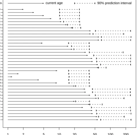
In this section, we present prediction intervals for the remaining life for individual transformers based on using the Weibull distribution and a stratification cutting at year 1987. Figure 2.4 shows 90% prediction intervals for remaining life for a subset of individual transformers that are at risk. The Years axis is logarithmic.

There are some interesting patterns in these results. In particular, for a group of relatively young transformers in the same group (young relative to expected life) and

(49)

with the same values of the explanatory variable(s), the prediction intervals are similar (but not exactly the same because of the conditioning on actual age). For a unit in such a group (i.e., one that has been in service long enough to have its age fall within the prediction intervals for the younger units), however, the lower endpoints of the interval are very close to the current age of the unit. Intervals for such units can be rather short, indicating that, according to our model, they are at high risk to failure. See, for example, unit MA New200 in Figure 2.4. Interestingly, as we were finishing this work, we learned of a recent failure of a transformer that had such a prediction interval.

Units, like MA New200, that are predicted to be at especially high risk for failure in the near term are sometimes outfitted with special equipment to continuously (hourly) monitor, communicate, and archive transformer condition measurements that are useful for detecting faults that may lead to failure. These measurements are taken from the transformer insulating oil and most commonly indicate the presence of dissolved gases but also may indicate other attributes including moisture content and loss of dielectric strength. Dissolved gas analysis (DGA) is automatically-performed by these monitors and is important in the transformer maintenance process, because it can be used to predict anomalous and dangerous conditions such as winding overheating, partial dis-charge, or arcing in the transformer. Without such a monitor, DGA is performed by sending an oil sample to a laboratory. These lab tests are routinely performed on a 6-12 month basis for healthy transformers but more frequently if a test indicates a potential problem. If an imminent failure can be detected early enough, the transformer can be operated under reduced loading until replaced, to avoid costly catastrophic failures that sometimes cause explosions. Lab testing, although generally useful, exposes the trans-former to possible rapidly deteriorating failure conditions between tests. Continuous monitoring eliminates this exposure but incurs the investment price of the monitoring equipment. Although this price is typically less than 1% of the transformer cost, the large number of transformers in a company’s fleet prohibits monitoring of all of them.

(50)

Years 1 2 5 10 20 50 100 200 ME_Old225 ME_Old555 ME_Old480 ME_Old696 ME_Old452 ME_Old635 ME_New380 Other_Old657 Other_Old125 Other_Old217 Other_Old596 Other_New612 Other_New174 Other_New548 Other_New236 Other_New361 Other_New387 MC_Old563 MC_Old422 MC_Old651 MC_Old115 MC_Old502 MC_Old554 MC_New364 MC_New568 MC_New644 MB_Old602 MB_Old170 MB_Old591 MB_Old527 MA_New200 MA_New243 MA_New535 MA_New182 MA_New597 MA_New521 MA_New183

Serial No. current age 90% prediction interval

Figure 2.4 Weibull distribution 90% prediction intervals for remaining life for a subset of individual at-risk transformers