The Beta-Hyperbolic Secant (BHS) Distribution

econ

stor

www.econstor.eu

Der Open-Access-Publikationsserver der ZBW – Leibniz-Informationszentrum Wirtschaft

The Open Access Publication Server of the ZBW – Leibniz Information Centre for Economics

Nutzungsbedingungen:

Die ZBW räumt Ihnen als Nutzerin/Nutzer das unentgeltliche, räumlich unbeschränkte und zeitlich auf die Dauer des Schutzrechts beschränkte einfache Recht ein, das ausgewählte Werk im Rahmen der unter

→ http://www.econstor.eu/dspace/Nutzungsbedingungen nachzulesenden vollständigen Nutzungsbedingungen zu vervielfältigen, mit denen die Nutzerin/der Nutzer sich durch die erste Nutzung einverstanden erklärt.

Terms of use:

The ZBW grants you, the user, the non-exclusive right to use the selected work free of charge, territorially unrestricted and within the time limit of the term of the property rights according to the terms specified at

→ http://www.econstor.eu/dspace/Nutzungsbedingungen By the first use of the selected work the user agrees and declares to comply with these terms of use.

zbw

Fischer, Matthias J.; Vaughan, David

Working Paper

The Beta-Hyperbolic Secant (BHS)

Distribution

Diskussionspapiere // Friedrich-Alexander-Universität Erlangen-Nürnberg, Lehrstuhl für Statistik und Ökonometrie, No. 64/2004

Provided in cooperation with:

Friedrich-Alexander-Universität Erlangen-Nürnberg (FAU)

Suggested citation: Fischer, Matthias J.; Vaughan, David (2004) : The Beta-Hyperbolic Secant (BHS) Distribution, Diskussionspapiere // Friedrich-Alexander-Universität Erlangen-Nürnberg, Lehrstuhl für Statistik und Ökonometrie, No. 64/2004, http://hdl.handle.net/10419/29617

Mar 2007

The Beta-Hyperbolic Secant (BHS) Distribution

Matthias J. Fischer1_{, David Vaughan}2

1 _{Department of Statistics. University of Erlangen-N¨urnberg, N¨urnberg, Germany} 2 _{Department of Mathematics, Wilfrid Laurier University, Waterloo, Ontario, Canada}

Abstract The shape of a probability distribution is often summarized by the distribution’s skewness and kurtosis. Starting from a symmetric ”par-ent” densityf on the real line, we can modify its shape (i.e. introduce skew-ness and in-/decrease kurtosis) iff is appropriately weighted. In particular, every densitywon the interval (0,1) is a specific weighting function. Within this work, we follow up a proposal of Jones (2004) and choose the Beta dis-tribution as underlying weighting function w. ”Parent” distributions like the Student-t, the logistic and the normal distribution have already been investigated in the literature. Based on the assumption that f is the den-sity of a hyperbolic secant distribution, we introduce the Beta-hyperbolic secant (BHS) distribution. In contrast to the Beta-normal distribution and the to Beta-Student-t distribution, BHS densities are always unimodal and all moments exist. In contrast to the Beta-logistic distribution, the BHS distribution is more flexible regarding the range of skewness and leptokur-tosis combinations. Moreover, we propose a generalization which nests both the Beta-logistic and the BHS distribution. Finally, the goodness-of-fit be-tween all above-mentioned distributions is compared for glass fibre data and aluminium returns.

1 Introduction

Several techniques can be applied to symmetric distributions in order to generate asymmetric ones with possibly lighter or heavier tails. In terms of density functions — provided their existence — most of these methods can be represented by

g(x;θ) =f(x)w(F(x);θ), (1)

wheregdenotes the transformed density,f andF the (symmetric) pdf and cdf, respectively, of the original (”parent”) distribution andwis an appro-priate weighting function on the interval (0,1) with parameter vectorθ(see, for instance, Ferreira and Steel, 2004). Choosingw(u;λ) = 2F(λF−1_(u)),

the skewing mechanism of Azzalini (1985, 1986) is recovered. Similarly, us-ing w(u;λ) = 2 λ+ 1 λ f(λsign(0.5−u)_F−1_(u)) f(F−1_(u)) (2)

corresponds to applying different parameters of scale to the positive and the negative part of a symmetric density (see, for example, Fern´andez, Osiewal-ski and Steel, 1995 and Theodossiou, 1998).

In particular, every probability density on (0,1) which is not uniform can be used either to introduce skewness and/or to modify the kurtosis of

the parent distribution. A very attractive choice (due to its flexibility) is the density of a Beta distribution, i.e.

w(x;β1, β2) = 1

B(β1, β2)x

β1−1_(1−x)β2−1_{, β}

1, β2>0, (3)

where B(a, b) = R₀1ta−1_(1−t)b−1_{dt denotes the Beta function (cf. Jones,}

2004). Examples where (3) has been used in the literature are the following:

– Aroian (1941), Prentice (1975): Beta-logistic distribution (which is also termed as exponential generalized beta of the second kind or EGB2 distribution, or logF distribution),

– Eugene et al. (2002): Beta-normal (BN) distribution,

– Jones and Faddy (2003): Beta-Student-t distribution.

Within this work we introduce the BHS (Beta-hyperbolic secant) distrib-ution as a weighted hyperbolic secant distribdistrib-ution with weights from (3). The hyperbolic secant distribution itself dates back to Perks (1932). It is symmetric, more leptokurtic than the normal, even more than the logistic distribution but still with existing moments. Both the cumulative distribu-tion funcdistribu-tion and the inverse cumulative distribudistribu-tion funcdistribu-tion are given in closed form. Despite its interesting properties, the hyperbolic secant distri-bution has not received sufficient attention in the literature so far.

Whereas both Beta-normal and Beta-Student-t distribution do not guar-antee unimodality — except for a special parameterization given in Ferreira and Steel (2004) — the BHS distribution does. In contrast to the Beta-Student-t distribution, all moments of the BHS distribution exist. Although the Beta-logistic and the BHS distribution are very similar, the BHS dis-tribution will be seen to be more flexible regarding skew and leptokurtic data. In order to discriminate between both distribution models, a gener-alized Beta-GSH model — based on Vaughan’s (2002) genergener-alized secant hyperbolic (GSH) distribution — is proposed that includes both candidate distributions as special case.

The paper is structured as follows: The BHS distribution and some fun-damental properties are introduced in section 2. Section 3 is devoted to the parameter estimation of the BHS distribution. A generalization of both the Beta-logistic distribution and the BHS distribution is proposed in section 4. In section 5, the BHS distribution is compared with its competitors derived from alternative parent distributions.

2 Definition and Properties

2.1 Definition of the Beta-Hyperbolic Secant Distribution

The probability density function of a standardized (i.e. zero mean and unit variance) hyperbolic secant distribution is given by

f(x) = 1

πcosh(x) =

2

π(ex_+e−x₎, x∈R. (4)

It is symmetric and the corresponding cumulative distribution function is

F(x) =2 arctan(e

x₎

π . (5)

The inverse cumulative distribution function is F−1_{(u) = log(tan(}πu

2 )).

Combining (1), (3), (4) and (5), the density of the Beta-hyperbolic secant (BHS) distribution is defined by g(x;β1, β2) = B(β1, β2) −1 πcosh(x) £₂ πarctan(exp(x)) ¤β1−1 £ 1− 2 πarctan(exp(x)) ¤1−β2, (6)

where β1 > 0 andβ2 > 0 determine the shape of the density. The

corre-sponding cumulative distribution function is

G(x;β1, β2) = BF−1_(x)(β₁, β₂) B(β1, β2) with Bu(p, q) = Z _u 0 tp−1(1−t)q−1dt.

Introducing a location parameter µ∈Rand a scale parameter σ >0, the BHS density from (6) generalizes to

g(x) = B(β1, β2)−1 σπcosh(x−_σµ) · 2 πarctan(e x−µ σ ) ¸β1−1 · 1− 2 πarctan(e x−µ σ ) ¸β2−1 .

Different densities and their corresponding log-densities with µ= 0, σ= 1 and varyingβ1, β2 are plotted in figure 1.

−4 −3 −2 −1 0 1 2 3 4 0 0.05 0.1 0.15 0.2 0.25 0.3 0.35 0.4 β₂=3 β₂=2 β2=1.25 β2=1 (a) Density −4 −3 −2 −1 0 1 2 3 4 −12 −10 −8 −6 −4 −2 0 β₂=1 β2=1.25 β2=2 β₂=3 (b) Log-density Fig. 1.Density and log-density forβ1= 1

Defineθ≡ β1−β2

2 andβ ≡

β1+β2

2 >0. Thenβ+θ=β1andβ−θ=β2, and

equation (3) can be rewritten as

w(x;β, θ) = 1 B(β+θ, β−θ)x β+θ−1_(1−x)β−θ−1 =C(β, θ)·xβ−1(1−x)β−1 B(β, β) · sin(πθ)xθ_(1−x)−θ πθ , (7)

where C(β, θ) = 1 only ifβ = 1. Thus, the weighting density can be par-titioned into two parts, where the first part essentially governs the amount of kurtosis and the second part the amount of skewness (see figure 2, where both parts are plotted separately). Consequently, a second parameterization of BHS density is given by g(x) = 1 πcosh(x) B(β+θ, β−θ) · 2 arctan(ex₎ π ¸β+θ−1 · 1−2 arctan(ex) π ¸β−θ−1 ,

(a) Kurtosis part (b) Skewness part Fig. 2.Decomposition of the weighting density

In order to ensure the existence of the Beta function in the last equation, bothβ+θandβ−θhave to be positive. Hence, it is required that|θ|< β, i.e. highly leptokurtic data (that means smallβ) induce higher restrictions onθ. It also becomes obvious from the above parameterization thatβ1 and

β2 commonly determine skewness and kurtosis (measured by the third and

fourth standardized moment within this work).

2.2 Properties of the BHS distribution

Lemma 1 (Asymmetry and kurtosis). The BHS distribution with

pa-rametersµ, σ, β1, β2 is symmetric about µforβ ≡β1=β2. Moreover, it is

skewed to the right forβ1> β2 and skewed to the left for β1< β2. Assume

that β1=β2≡β. Then, kurtosis increases ifβ decreases and vice versa.

Lemma 2 (Tail behavior). The BHS distribution has exponentially

de-caying tails. In particular, the log-density is asymptotically linear with slope determined byβ1 andβ2, respectively.

Proof. Assumeµ= 0,σ= 1 and focus on the right tail of the BHS

distrib-ution. From lim x→∞ µ 1 cosh(x)−2 exp(−x) ¶ = 0, lim x→∞ · 2 πarctan(e x₎ ¸β1−1 = 1, and · 1−2 πarctan(e x₎ ¸β2−1 ∼ Cexp((1−β2)x)

we conclude that for largex

g(x;β1, β2) ∼ Cexp(−x) exp((1−β2)x) =Cexp(−β2x), C= (2/π)

β2

B(β1, β2).

In particular,β2 <1 corresponds to distributions with heavier than plain

exponential tails,β2 >1 distributions with lighter than plain exponential

tails. The same argument is true for the left tail.

Additionally, the score function for the BHS distribution is derived which plays an important role in the theory of rank test (see, e.g. Kravchuk, 2005, forβ1=β2= 1)

Lemma 3 (Score function). With ζ(x)≡arctan (ex_{) the score function}

of a BHS variable is given by ψ(x;β1, β2) =− g0_(x;β 1, β2) g(x;β1, β2) = tanh (x)ζ(x)(e 2x_{+ 1)(2ζ(x)−π) +e}x_β 1(π−2ζ(x)) (1 +e2x_{)ζ(x) (2ζ(x)−π)} − e x_π−2ex_ζ(x)(2−β 2) (1 +e2x_{)ζ(x) (2ζ(x)−π)}.

Settingβ1=β2= 1, the last equation reduces toψ(x; 1,1) = tanh(x).

Finally, it can be shown (see Appendix A for a detailed proof) that BHS densities are unimodal for all β1, β2 > 0. This is not valid for the

Beta-normal and the Beta-Student-t distribution, in general.

Lemma 4 (Unimodality).The BHS distribution is unimodal forβ1, β2>

0.

2.3 Special and limiting cases

First of all, forβ1=β2= 1 the hyperbolic secant distribution is recovered.

Setting β2 = 1 or β1 = 1, skew hyperbolic secant distributions can be

obtained. A generalized symmetric family of hyperbolic secant distributions is achieved forβ1=β2=β, whereβ governs the amount of kurtosis. Like

the Beta-logistic distribution and the Beta-normal distribution, the BHS distribution converges to the normal distribution forβ1, β2→ ∞.

2.4 Moments of the BHS distribution

Obviously, the exponential tail behaviour of the BHS distribution guaran-tees the existence of all moments. In particular, themth_{non-central moment}

of a BHS density is given by E(Xm) = 1 B(β1, β2) Z ₁ 0 lnm(tan(π 2u))u β1−1_(1−u)β2−1_du.

From Gradshteyn and Ryhzik (1994), formula 1.518.3 and 9.616 we can write tan(π 2u) = ln( π 2u) + ∞ X k=1 (22k−1_−1)ζ(2k) k22k−1 u 2k_{= ln(}π 2u) +u 2 ∞ X k=0 aku2k

with the usual Riemann zeta function ζ(2k) = ∞ X l=1 1 l2k andak = (22k+1_{−1)ζ(2k+ 2)} (k+ 1)22k+1 . (8)

Using the notation ∂v

∂pvB(p, q)≡B

v,0_{(p, q), B}0,0_{(p, q) =B(p, q),}

the following lemma can be derived.

Lemma 5 (Moments of the BHS distribution). Assume thatm >0.

E(Xm_{) =} 1 B(β1, β2)   m X j=0 µ m j ¶ lnm−j(π 2)B j,0_(β 1, β2)+ + ∞ X k=0 m X j=1 µ m j ¶ a(_kj) m_X−j i=0 µ m−j i ¶ lnm−j−i(π 2)B i,0_{(2k+ 2j+β} 1, β2)  _, where a(₀j)=aj₀, a(_kj)= 1 ka0 k X i=1 (ij−k+i)aia(_kj₋)_i, k≥1.

In particular, the mean of the BHS distribution is given by E(X) = ln(π 2) +ψ(β1)−ψ(β1+β2) + ∞ X k=0 akB(2k+ 2 +β1, β2) B(β1, β2) . (9)

with ak from (8). Note that ψ denotes the digamma function in the last

equation. In contrast to (9), the corresponding formula for the Beta-logistic distribution is given by

E(X) =ψ(β1)−ψ(β2).

From the first four moments we can deduce the skewness and kurtosis co-efficients M3 andM4 (i.e the third and fourth standardized moments) for

different parameter combinations of the BHS distribution. 2.5 Moment ratio diagrams

Moment ratio diagrams have been introduced for Pearson-type distributions by Elderton and Johnson (1969) in order to provide a useful visual assess-ment of skewness and kurtosis. The classical moassess-ment ratio plot consists of all possible pairs (M3, M4) that can be obtained through different

combi-nations of the shape parameters of the underlying distributions. In general, the relationM2

3 < M4−1 forM4>0 holds, i.e. for a given level of kurtosis

only a finite range of skewness may be spanned.

Due to the bi-modality of the Beta-normal distribution and the

non-existence of some moments for the Beta-Student-t distribution we only

compare the BHS distribution with the Beta-logistic (EGB2) distribution in figure 3, below.

(a) EGB2 distribution

(b) BHS distribution Fig. 3.Moment ratio diagrams

The possible combinations of skewness and kurtosis (for a given dis-tribution) are indicated by the black area which was generated using a

large number of random numbers from the domain of the shape parameters (β1, β2). The dashed line (encompassing the black area) corresponds to the

boundary mentioned above. Note that we plotted theexponentiatedkurtosis against the skewness in order to highlight the differences between EGB2 dis-tribution and BHS disdis-tribution. It then becomes visible that the achievable area of the BHS distribution includes that of the EGB2 distribution.

3 Parameter estimation using maximum likelihood

Suppose thatX1, . . . , Xnare aniidrandom sample from a BHS distribution.

Introducing a scale parameter σ >0 and a location parameterµ∈R, the log-likelihood function is given by

`(θ) =nlog µ (2/π)β1+β2−2 B(β1, β2)πσ ¶ + n X i=1 {(β1−1) log(arctan(exp(x∗i))) +(β2−1) log ³_π 2 −arctan(exp(x ∗ i)) ´ −log(cosh(x∗i)) o . wherex∗

i = (xi−µ)/σand θ= (µ, σ, β1, β2). Taking the partial derivative

of the log-likelihood with respect to the parametersµ, σ, β1, β2 we obtain

0 = ∂` ∂µ= 1 σ n X i=1 µ tanh(x∗ i) + (1−β1) exp(x∗i) (1 +e2x∗ i) arctan(ex∗i) + (β2−1) exp(x ∗ i) (1 +e2x∗ i)(π/2−arctan(ex∗i)) ¶ , 0 = ∂` ∂σ =− à (2/π)b1+b2−2 B(β1, β2)πσ !n n σ + 1 σ2 n X i=1 (xi−µ) µ tanh(x∗i) + (1−β1) exp(x∗i) (1 +e2x∗ i) arctan(ex∗i) + (β2−1) exp(x∗i) (1 +e2x∗ i)(π/2−arctan(ex∗i)) ¶ 0 = ∂` ∂β1 = n 4n à ¡₂ π ¢β1+β2 π B(β1, β2)σ !n_µ log µ 2 π ¶ −B (1,0)_(β 1, β2) B(β1, β2) ¶ + n X i=1 log(arctan(exp(x∗ i))),

0 = ∂` ∂β2 = n 4n à ¡₂ π ¢β1+β2 π B(β1, β2)σ !n_µ log µ 2 π ¶ −B(0,1)(β1, β2) B(β1, β2) ¶ + n X i=1 log(π/2−arctan(exp(x∗i))).

We solve the equations above iteratively to obtain ˆβ1,βˆ2,µ,ˆ σ.ˆ

4 Generalizations: EGB2 versus BHS distribution

In order to discriminate between Beta-logistic (EGB2) and BHS distribu-tion we can plug a parent distribudistribu-tion into (3) which includes both logistic distribution and hyperbolic secant distribution. A promising choice is the GSH distribution of Vaughan (2002) with kurtosis parametertand density

fGSH(x;t) =c1(t)· exp(x)

exp(2x) + 2a(t) exp(x) + 1, x∈R (10)

with

(

a(t) = cos(t), c1(t) = sin(_tt) for −π < t≤0,

a(t) = cosh(t), c1(t) = sinh(_t t) fort >0

.

The GSH distribution includes the logistic distribution (t= 0) and the hy-perbolic secant distribution (t=−π/2) as special cases and has cumulative distribution function given by

FGSH(x;t) =          1 + 1 tarccot ³

−exp(_sin(x)+cos(_t) t)

´ fort∈(−π,0), exp(πx/√3) 1+exp(πx/√3) fort= 0, 1−1 tarccoth ³ exp(x)+cosh(t) sinh(t) ´ fort >0. Thus, we can apply a simple likelihood ratio test to the hypothesis

5 Applications

5.1 Strength of glass fibre

Our first example corresponds to that of Jones and Faddy (2003) who ana-lyzed the strengths of glass fibre. This data set is ’sample 1’ of Smith and Naylor (1987) and deals with the breaking strength ofn= 63 glass fibres of length 1.5 cm, originally obtained by workers at the UK National Physical Laboratory. Due the apparent skewness in the data set (see figure 4(a) for a histogram of the data), Jones and Faddy (2003) fitted a Beta-Student-t distribution – using a reparameterized version – to the data, estimating the unknown parameters by means of maximum likelihood.

(a) Histogram (b) Fitted densities

Fig. 4.Strength of glass fibre

Additionally, we fitted a normal, a logistic (EGB2), a Beta-hyperbolic secant (BHS) and a Beta-GSH distribution to the data. The estimation results are summarized in table 1, below. Graphs of the fitted densities are provided by figure 4(b).

Regarding the log-likelihood valueL, the Beta-normal distribution seems to fit worse. Both Beta-logistic and Beta-hyperbolic secant distribution outperform the Beta-Student-t distribution, in particular, if we account for the number of parameters k and focus on the criterion of Akaike, i.e. AIC =−2L+ 2k. Moreover, the log-likelihood value of the BHS distribu-tion is higher than that of the EGB2 distribudistribu-tion. Finally, the Beta-GSH distribution provides evidence in favor of the BHS distribution against the EGB2 distribution.

Table 1.Estimation results for the glass fibre data set . Distribution µb bσ βb1 βb2 bν/bt L AIC Normal 1.51 [0.0409] [00..0287]322 - - - −17.91 39.82 Beta-Normal 2.60 [0.2005] [00..1558]475 0[0.5946.37] [423.7340].66 - −14.06 36.11 Beta-Logistic 1.67 [0.0460] [00..0393]041 0[0.1450.14] [00.3085].31 - −10.49 28.99 BHS 1.65 [0.0400] [00..0662]043 0[0.1451.23] [00.4638].28 - −10.02 28.03 Beta-Student-t 1.70 [0.0695] [00..2099]621 49[43.345.4] [4656..484]83 [00.0688].12 −11.41 32.82 Beta-Student-t2 1.70 [0.0763] [00..0958]226 1[0.1073.60] [12.1947].08 −11.93 33.86 Beta-GSH 1.65 [0.0383] [00..0861]071 0[0.2270.26] [00.4761].43 [0−.25939].00 −9.90 29.80

Concerning the estimation results of the Student-t, the parametersβ1, β2, ν

seem to be poorly identified. We therefore fix the number of degrees at 2 as in Jones and Faddy (2003). Note that the 6th column of table 1 contains the estimated shape parameter beyondβb1andβb2, i.e. the estimated degrees

of freedom bν for a Beta-Student-t distribution and the estimated t of the Beta-GSH distribution, respectively.

5.2 Returns aluminium

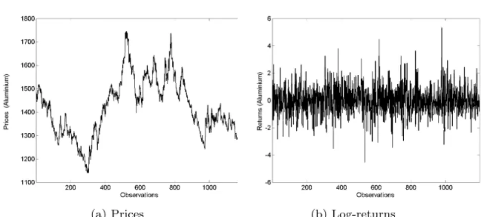
Secondly, we focus on the series of the daily aluminium prices (in

US-Dollar/Tonne) from January 1999 to September 2002 (N = 1195

obser-vations) which can be obtained from the LME (London Metal Exchange).1

The series of prices and corresponding log-returns (i.e. difference of consec-utive log-prices) are displayed in figure 5.

The (sample) mean of the log-returns is−0.0139 with a (sample) standard deviation of 1.0560. Moreover, there seems to be a certain amount of skew-ness in the data set (the skewskew-ness coefficient – measured by the third stan-dardized moments – is given by by 0.2398), whereas the kurtosis coefficient – in terms of the fourth standardized moments – is 4.4250, reflecting the leptokurtosis of the data. The results of a maximum likelihood estimation are summarized in table 2, below.

(a) Prices (b) Log-returns Fig. 5.Prices and log-returns of aluminium 05/01/98 to 30/09/02

Table 2.Unconditional fit to the aluminium returns

Distribution µb σb βb1 βb2 ν/bbt L AIC Normal −0.014 [0.031] [01..056022] - - - −1758.8 3521.5 Beta-Normal −1.218 [0.697] [01..728586] [33..980058] [01..520792] - −1753.0 3514.0 Beta-Logistic −0.248 [0.087] [00..497091] [00..932243] [00..719182] - −1733.6 3475.2 BHS −0.282 [0.099] [00..921156] [01..738445] [01..355336] - −1733.5 3474.9 Beta-Student-t −0.331 [0.167] [33..874310] [12849.65.1] [12647.013.384] [00..473]26 −1734.0 3478.0 Beta-Student-t2 −0.294 [0.285] [01..643563] [33..804013] [23..146171] −1734.3 3478.7 Beta-GHS −0.286 [0.089] [00..966895] [11..819517] [11..419285] −[1.1026].63 −1733.5 3476.9

Though this data set is totally different to the glass fibre data, the results are nearly identical (concerning the order of the log-likelihood val-ues). Again, the Beta-GSH distribution favors the BHS distribution against the Beta-Logistic distribution with bt = −1.63, both of which outperform normal and Student-t. Again, the shape parameters of the Beta-Student-t seem to be unidentified.

6 Summary

A new class of probability densities (the so-called BHS-distribution family) is introduced which arises as special case from the general family explored by Jones (2004) if the hyperbolic secant distribution is chosen as ”parent distribution”. It exhibits similar behavior and properties like the log-F or EGB2 distribution. In particular, the range of possible skewness and kur-tosis combinations of the BHS distribution includes that of the EGB2 dis-tribution. Moreover, a generalized distribution model is introduced which includes both EGB2 and BHS distribution. Application to glass fibre data and aluminium returns provides empirical evidence in favor of the BHS distribution.

7 Appendix: Proof of uni-modality

In the Jones and Faddy formulation, the density function for a family of Skew Generalized Secant Hyperbolic Distributions is given by

g(x) = 1

B(β1, β2)f(x)[F(x)]

a_[1−F(x)]b

where f(x) = 1

πcosh(x) so that F(x) = 2/πarctan(exp(x)), and we assume

a, b > −1. We want to show this density is unimodal for all choices of a and b. Since the functions are all continuous and continuously differen-tiable, the only critical points for the functiong satisfyg0_{(x) = 0. Thus we}

want to prove that this has exactly one root, and that this yields a relative maximum. Since limx→±∞g(x) = 0, then if there is one critical point, it

must yield the absolute maximum, so we need to prove there is exactly one root to the derivative equation. After simplification, this can be seen to be equivalent to proving −sinh(x) + a 2 tan−1_(exp(x))− b π(1− 2 πtan−1(exp(x)) = 0

has exactly one root. Note that if we setu= tan−1_{(exp(x)), the last}

state-ment is equivalent to showing

−(tan(u)−cot(u))u(π/2−u) =−πa

2 + (a+b)u

has exactly one root in (0, π/2). Define

h(u) =−(tan(u)−cot(u))u(π/2−u)

on (0, π/2). Note that h(u+π/4) is odd on (−π/4, π/4). Also,h(π/4) = 0 and we set h(0) = limu→0+h(u) =π/2, andh(π/2) = limu→(π/2)−h(u) =

−π/2. Note that

h0_{(u) =−} u(π/2−u)

sin2(u) cos2_(u)−(tan(u)−cot(u))(π/2−2u)

and

h00_{(u) =} 4

sin3(2u)[4 cos(2u)u(π/2−u)−2 sin(2u)(π/2−2u)−cos(2u) sin

2_(2u)].

We want to prove that his concave down on (0, π/4) and concave up on

(π/4, π/2). The second fact will follow from the first, and the symmetry property of h noted earlier. Thus, we want to prove that h00_{(u) < 0 on}

(0, π/4). By using trigonometric identities, we can show this is equivalent to proving the functionk(v) =v(π−v) cosv−2(π/2−v) sinv−cosvsin2v <0

on (0, π/2). Now k(0) = 0, k(π/2) = 0. Note that k0_{(v) = sinv[v}2_−πv+

3 sin2_(v)].

Set z(v) = 3 sin2v+v2_{−πv, and note that z(0) = 0 and z(π/2) =}

3−π2_{/4>0. We havez}0_{(v) = 3 sin(2v) + 2v−πandz}00_{(v) = 6 cos(2v) + 2.}

Clearly, z00 _{> 0 if cos(2v) > −1/3 and z}00 _{< 0 if cos(2v) < −1/3. In the}

interval (0, π/2) there is a unique value, sayα0so that cos(2α0) =−1/3 and

hence on (0, α0),z00(v)>0 and on (α0, π/2),z00(v)<0. Becausez0(0) =−π

andz0_{(π/2) = 0, there is a unique valueα}

1∈(0, α0) for whichz0(α1) = 0.

We then have z0_{(v) < 0 on (0, α}

1) and z0(v) > 0 on (α1, π/2). From the

valuesz(0) = 0 and z(π/2)>0, and the properties ofz0_{, there is a unique}

valueα2∈(0, π/2) for whichz(α2) = 0.

The above shows that k0 _{has exactly one root in (0, π/2), call it β}

0. It

is clear that k0_{(v)<0 on (0, β}

0), andk0(v)>0 on (β0, π/2). This in turn

impliesk(v)<0 on (0, π/2), sincek(0) = 0 =k(π/2).

The above argument establishes that h00_{(u)<0 on (0, π/4), and}

there-fore h is concave down on (0, π/4) and concave up on (π/4, π/2). Set

w(u) = −πa

2 + (a+b)u on (0, π/2). Since w(0) = −πa2 < h(0) = π/2

andw(π/2) = πb

2 > h(π/2) =π/2, then wand hintersect. If these curves

intersect on (0, π/4), they cannot intersect a second time on (0, π/4) (oth-erwise, since h is concave down, the line through the intersection points cannot intersectha third time on this interval. This means the vertical axis intercept for the line is> π/2, and this is not possible, given the line must intersect the vertical axis at (0,−πa

2 )). Further, the linewcannot intersect

hon (π/4, π/2) in this case, since w’s slope is greater than −2, and −2 is the slope of the liney =π/2−2ujoining the points (0, π/2), (π/4,0) and (π/2,−π/2) onh. Hencewandy have a unique intersection point, so that if w intersects h on (π/4, π/2), this will force w and y to intersect again, a contradiction. A similar analysis shows that if w and h do intersect on (π/4, π/2), they do so uniquely, and do not intersect on (0, π/4).

Altogether, this means thatg0 _{has exactly one root in (−∞,∞). It then}

also follows this yields a relative maximum (and hence absolute maximum) sinceg0 _{is positive to the left of the root, and negative to the right.2}

References

Aroian LA (1941) A Study of R. A. Fisher’s z Distribution and the Related f Distribu-tion. Annals of Mathematical Statistics12: 429-448

Azzalini A (1985) A Class of Distributions which includes the Normal Ones. Scandina-vian Journal of Statistics12: 171-178.

Azzalini A (1986) Further Results on a Class of Distributions which includes the Normal Ones. Statistica46: 199-208.

Elderton WP, Johnson NL (1969)Systems of Frequency Curves. Addison Wesley, Read-ing.

Fern´andez C, Osiewalski J, Steel MFJ (1995) Modelling and Inference withν-spherical Distributions. Journal of the American Statistical Society90: 1331-1340.

Eugene N, Lee C, Famoye F (2002) Beta-Normal Distribution and its Applications. Communications in Statistics, Theory and Methods31(4): 497-512.

Ferreira JTAS, Steel, MFJ (2004) A Constructive Representation of Univariate Skewed Distributions. Working Paper, Department of Statistics, University of Warwick. Gradshteyn IS, Ryhzik IM (1994)Tables of Integrals, Series, and Products. Academic Press, New York.

Jones MC (2004) Families of Distributions Arising from Distributions of Order Statis-tics. Test13(1): 1-43.

Jones MC, Faddy, MJ (2004) A Skew Extension of the t-distribution, with Applications. Journal of the Royal Statistical Society, Series B65(1): 159-174.

Kravchuk, OY (2005) Rank Test of Location Optimal for Hyperbolic Secant Distribu-tion. Communications in Statistics (Theory and Methods),34(7): 1617-1630.

Perks, WF (1932) On Some Experiments in the Graduation of Mortality Statistics. Institute of Actuaries Journals, Series B58: 12-57.

Prentice RL (1975) Discrimination among some Parametric Models. Biometrika 62: 607-614.

Smith RL, Naylor JC (1987) A Comparison of Maximum Likelihood and Bayesian Estimators for the Three-Parameter Weibull Distribution. Applied Statistics36(3): 358-369.

Theodossiou P (1998) Financial data and the skewed generalized t distribution. Math-ematical Science44(12): 1650-1660.

Vaughan DC (2002) The Generalized Hyperbolic Secant Distribution and its Applica-tion. Communications in Statistics, Theory and Methods31(2): 219-238.