Learning Robust Representations via Multi-View Information Bottleneck

LEARNING

ROBUST

REPRESENTATIONS VIA

MULTI-VIEW

INFORMATION

BOTTLENECK

Marco Federici University of Amsterdam [email protected] Anjan Dutta University of Exeter [email protected] Patrick Forr´e University of Amsterdam [email protected] Nate Kushmann

Microsoft Research Cambridge [email protected]

Zeynep Akata University of T¨ubingen

[email protected]

A

The information bottleneck method Tishby et al. (2000) provides an information-theoretic method for representation learning, by training an encoder to retain all in-formation which is relevant for predicting the label, while minimizing the amount of other, superfluous information in the representation. The original formulation, however, requires labeled data in order to identify which information is superflu-ous. In this work, we extend this ability to the multi-view unsupervised setting, in which two views of the same underlying entity are provided but the label in unknown. This enables us to identify superfluous information as that which is not shared by both views. A theoretical analysis leads to the definition of a new multi-view model which produces state-of-the-art results on the Sketchy dataset and on label-limited versions of the MIR-Flickr dataset. We also extend our the-ory to the single-view setting by taking advantage of standard data augmentation techniques, empirically showing better generalization capabilities when compared to traditional unsupervised approaches for representation learning.

1

I

The goal of deep representation learning (LeCun et al., 2015) is to transform a raw observational input,x, into a representation,z, to extract useful information. Significant progress has been made in deep learning via supervised representation learning, where the labels, y, for the downstream task are known whilep(y|x)is learned directly (Sutskever et al., 2012; Hinton et al., 2012). Due to the cost of acquiring large labeled datasets, a recently renewed focus on unsupervised represen-tation learning seeks to generate represenrepresen-tations,z, that allow learning of (a priori unknown) target supervised tasks more efficiently, i.e. with fewer labels (Devlin et al., 2018; Radford et al., 2019). Our work is based on the information bottleneck principle (Tishby et al., 2000) stating that whenever a data representation discards information from the input which is not useful for a given task, it becomes less affected by nuisances, resulting in increased robustness for downstream tasks. In the supervised setting, one can directly apply the information bottleneck method by minimizing the mutual information betweenzandxwhile simultaneously maximizing the mutual information betweenz andy (Alemi et al., 2017). In the unsupervised setting, discarding only superfluous information is more challenging as without labels one cannot directly identify the relevant informa-tion. Recent literature (Devon Hjelm et al., 2019; van den Oord et al., 2018) has instead focused on the InfoMax objectivemaximizingthe mutual information betweenxandz,I(x,z), instead of minimizing it.

In this paper, we extend the information bottleneck method to the unsupervised multi-view setting. To do this, we rely on a basic assumption of the multi-view literature – that each view provides the sametask relevant information(Zhao et al., 2017). Hence, one can improve generalization by discarding from the representation all information which is not shared by both views. We do this through an objective which maximizes the mutual information between the representations of the

two views (Multi-View InfoMax) while at the same time reducing the mutual information between each view and its corresponding representation (as with the information bottleneck). The resulting representation contains only the information shared by both views, eliminating the effect of inde-pendent factors of variations.

Our contributions are three-fold: (1) We extend the information bottleneck principle to the unsuper-vised multi-view setting and provide a rigorous theoretical analysis of its application. (2) We define a new model that empirically leads to state-of-the-art results in the low-data setting on two standard multi-view datasets, Sketchy and MIR-Flickr. (3) By exploiting standard data augmentation tech-niques, we empirically show that the representations obtained with our model in single-view settings are more robust than other popular unsupervised approaches for representation learning, connecting our theory to the choice of augmentation function class.

2

P

F

The challenge of representation learning can be formulated as finding a distributionp(z|x)that maps data observationsx∈Xinto a code spacez∈Z. Whenever the end goal involves predicting a label

y, we consider only thezthat are discriminative enough to identify the label. This requirement can be quantified by considering the amount of target information that remains accessible after encoding the data, and is known in literature as sufficiency ofzfory(Achille & Soatto, 2018):

Definition 1. Sufficiency: A representationzofxis sufficient foryif and only ifI(x;y|z) = 0 Any model that has access to a sufficient representationz must be able to predict y at least as accurately as if it has access to the original data x instead. In fact,z is sufficient for y if and only if the amount of information regarding the task is unchanged by the encoding procedure (see Proposition B.1 in the Appendix):

I(x;y|z) = 0 ⇐⇒ I(x;y) =I(y;z). (1) Among sufficient representations, the ones that result in better generalization for unlabeled data in-stances are particularly appealing. Whenxhas higher information content thany, some of the infor-mation inxmust be irrelevant for the prediction task. This can be better understood by subdividing I(x;z)into three components by using the chain rule of mutual information (see Appendix A):

I(x;z) = I(x;z|y) | {z } superfluous information + I(x;y) | {z } predictive information − I(x;y|z) | {z } predictive information not inz

. (2)

Conditional mutual informationI(x;z|y)represents the information inzthat is not predictive of y, i.e. superfluous information. While I(x;y)is a constant determined by how much label in-formation is accessible from the raw observations; the last termI(x;y|z)represents the amount of information regardingythat is lost by encodingxintoz. Note that this last term is zero whenever zis sufficient forx. Since the amount of predictive informationI(x;y)is fixed,

Proposition 2.1. A sufficient representationzofxforyis minimal wheneverI(x;z|y)is minimal. Minimizing the amount of superfluous information can be done directly only in supervised settings. In fact, reducingI(x;z) without violating the sufficiency constraint necessarily requires making some additional assumptions on the predictive task (see Theorem B.1 in the Appendix). In Section 3 we describe a strategy to safely reduce the information content of a representation even when the labelyis not observed, by exploiting redundant information in the form of an additional view on the data.

3

M

-V

I

B

Letv1andv2be two images of the same object from different view-points andybe its label.

As-suming that the object is clearly distinguishable from bothv1andv2, any representationzwith all

the information that is accessible from both views would also contain the necessary label informa-tion. Furthermore, ifzcaptures only the details that are visible from both pictures, it would reduce the total information content, discarding the view-specific details and reducing the sensitivity of the representation to view-changes. The theory to support this intuition is described in the following wherev1andv2are jointly observed and referred to as data-views.

3.1 SUFFICIENCY ANDROBUSTNESS IN THEMULTI-VIEW SETTING

In this section we extend our analysis of sufficiency and robustness to the multi-view setting. Intuitively, we can guarantee thatzis sufficient for predictingy even without knowingy by en-suring thatzmaintains all information which is shared by v1 andv2. This intuition relies on a

basic assumption of the multi-view environment – that each view provides the same task relevant information. To formalize this we defineredundancy.

Definition 2. Redundancy:v1is redundant with respect tov2foryif and only ifI(y;v1|v2) = 0

Intuitively, a viewv1is redundant for a task whenever it is irrelevant for the prediction ofywhen

v2is already observed. Wheneverv1andv2aremutually redundant(v1is redundant with respect

tov2fory, and vice-versa), we can show the following:

Corollary 1. Letv1andv2be two mutually redundant views for a targetyand letz1be a

repre-sentation ofv1. Ifz1is sufficient forv2(I(v1;v2|z1) = 0) thenz1is as predictive foryas the joint

observation of the two views (I(v1v2;y) =I(y;z1)).

In other words, whenever it is possible to assume mutual redundancy, any representation which contains all the information shared by both views (the redundant information) is as useful as their joint observation for predicting the labely.

By factorizing the mutual information betweenv1andz1analogously to Equation 2, we can identify

3 components: I(z1;v1) = I(v1;z1|v2) | {z } superfluous information + I(v1;v2) | {z } shared information − I(v1;v2|z1) | {z }

shared information not inz1 .

SinceI(v1;v2)is a constant that depends only on the two views andI(v1;v2|z1)must be zero if

we want the representation to be sufficient for the label, we conclude thatI(v1;z1)can be reduced

by minimizingI(v1;z1|v2). This term intuitively represents the informationz1contains which is

unique tov1and not shared byv2. Since we assumed mutual redundancy between the two views,

this information must be irrelevant for the predictive task and, therefore, it can be safely discarded. The proofs and formal assertions for the above statements and Corollary 1 can be found in Appendix B.

The less the two views have in common, the moreI(z1;v1)can be reduced without violating

suf-ficiency for the label, the more robust the resulting representation. At the extreme, v1 andv2

share only label information, in which case we can show thatz1is minimal foryand our method

is identical to the supervised information bottleneck method without needing to access the labels. Conversely, ifv1andv2are identical, then our method degenerates to the InfoMax principle since

no information can be safely discarded (see Appendix E).

3.2 THEMULTI-VIEWINFORMATIONBOTTLENECKLOSSFUNCTION

Givenv1andv2that satisfy the mutual redundancy condition for a labely, we would like to define

an objective function for the representationz1ofv1that discards as much information as possible

without losing any label information. In Section 3.1 we showed that we can maintain sufficiency for yby ensuring thatI(v1;v2|z1) = 0, and that decreasingI(z1;v1|v2)will increase the robustness

of the representation by discarding irrelevant information. So if we combine these two terms using a relaxed Lagrangian objective, then we obtain:

L1(θ;λ1) = Iθ(z1;v1|v2)

| {z }

superfluous information

+ λ1Iθ(v1;v2|z1)

| {z }

sufficiency ofz1for predictingy

, (3)

whereθ denotes the dependency on the parameters of the encoder pθ(z1|v1), and λ1 represents

the Lagrangian multiplier introduced by the constrained optimization. Symmetrically, we define a lossL2 to optimize the parametersψof a conditional distributionpψ(z2|v2)that defines a robust

sufficient representationz2of the second viewv2:

L2(ψ;λ2) = Iψ(z2;v2|v1)

| {z }

superfluous information

+ λ2Iψ(v1;v2|z2)

| {z }

sufficiency ofz2for predictingy

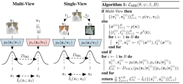
Multi-View Single-View v1 v2 pθ(z1|v1) pψ(z2|v2) ∼ ∼ z1 z2 DSKL ˆ Iξ(z1;z2) x v1 v2 pθ(z1|v1) pθ(z2|v2) ∼ ∼ z1 z2 DSKL ˆ Iξ(z1;z2) t1 t2 Algorithm 1:LMIB(θ, ψ;β, B) ifMulti-Viewthen {(v(1i),v (i) 2 )} B i=1∼p(v1,v2); else {x(i)}B i=1∼p(x); {(t(₁i), t(₂i))}B i=1∼p2(t); fori←1toBdo v₁(i),v₂(i)←t₁(i)(x(i)_{), t}(i) 2 (x (i)_); end for end if fori←1toBdo z1(i),z (i) 2 ∼pθ(z1|v(1i)), pψ(z2|v2(i)); L(mi)←DSKL(pθ(z1|v (i) 1 )||pψ(z2|v (i) 2 )); end for return_Bβ PB i=1L (i) m −Iˆξ({(z (i) 1 ,z (i) 2 )} B i=1)

Figure 1: Visualizing our Multi-View Information Bottleneck model for both multi-view and single-view settings. Wheneverp(v1)andp(v2)have the same distribution, the two encoders can share

their parameters.

AlthoughL1andL2can not be computed directly, by definingz1andz2on the same domainZand

re-parametrizing the Lagrangian multipliers, their sum can be upper bounded as follows:

LM IB(θ, ψ;β) =− Iθψ(z1;z2) | {z }

sufficiency ofz1andz2for predictingy

+β DSKL(pθ(z1|v1)||pψ(z2|v2))

| {z }

superfluous information

, (5) whereDSKLis the symmetrized KL divergence obtained by averagingDKL(pθ(z1|v1)||pψ(z2|v2))

andDKL(pψ(z2|v2)||pθ(z1|v1)), while the coefficientβdefines the trade-off between sufficiency

and robustness of the representation, which is a hyper-parameter in this work. The resulting Multi-View Infomation Bottleneck (MIB) model (Equation 5) is visualized in Figure 1, while the batch-based computation of the loss function is summarized in Algorithm 1.

The symmetrized KL divergenceDSKL(pθ(z1|v1)||pψ(z2|v2))can be computed directly

when-everpθ(z1|v1)andpψ(z2|v2)have a known density, while the mutual information between the two

representationsIθψ(z1;z2)can be maximized by using any sample-based differentiable mutual

in-formation lower bound. Both the Jensen-ShannonIJS(Devon Hjelm et al., 2019; Poole et al., 2019)

and the InfoNCEINCE(van den Oord et al., 2018) estimators used in this work require introducing

an auxiliary parameteric modelCξ(z1,z2), which is jointly optimized during the training procedure.

The full derivation for the MIB loss function can be found in Appendix F. 3.3 SELF-SUPERVISION ANDINVARIANCE

In this section, we introduce a methodology to build mutually redundant views starting from single observationsxwith domainXby exploiting known symmetries of the task.

By picking a class_Tof functionst : _X → _Wthat do not affect label information, it is possible to artificially build views that satisfy mutual redundancy fory with a procedure similar to data-augmentation. Lett1andt2be two random variables overT, thenv1 :=t1(x)andv2 :=t2(x)

must be mutually redundant fory. Since no function in_Taffects label information (I(v1;y) =

I(v2;y) =I(x;y)), a representationz1ofv1that is sufficient forv2must contain same amount of

predictive information asx. Formal proofs can be found in Appendix B.4.

Whenever the two transformations for the same observations are independent (I(t1;t2|x) = 0),

they introduce uncorrelated variations in the two views. As an example, if_Trepresents a set of small translations, the two views will differ by a small shift. Since this information is not shared,z1that

contains only common information betweenv1andv2will discard fine-grained details regarding

For single-view datasets, we generate the two views v1 and v2 by independently sampling two

functions from the same function classTwith uniform probability. Since the resultingt1andt2

have the same distribution, the two generated views will also have the same marginals. For this reason, the two conditional distributionspθ(z1|v1)andpψ(z2|v2)can share their parameters and

only one encoder can be used. Full (or partial) parameter sharing can be also applied in the multi-view settings whenever the two multi-views have the same (or similar) marginal distributions.

4

R

W

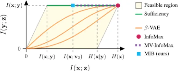
The space of all the possible representationszof xfor a predictive tasky can be represented as a region in the Information Plane (Tishby et al., 2000). Each representation is characterised by the amount of information regarding the raw observationI(x;z)and the corresponding measure of accessible predictive informationI(y;z)(xandy axis respectively on Figure 2). Ideally, a good representation would be maximally informative about the label while retaining a minimal amount of information from the observations (top left corner of the parallelogram). Further details on the Information Plane and the bounds visualized in Figure 2 are described in Appendix C.

0 0 I(x;y) H(x) I(x;y) I(x;v2) H(x|y) I ( y ; z ) I(x;z) Feasible region Sufficiency InfoMax MV-InfoMax β-VAE MIB (ours)

Figure 2: Information Plane determined by I(x;z)(x-axis) andI(y;z)(y-axis). Different ob-jectives are compared based on their target. Thanks to recent progress in mutual

informa-tion estimainforma-tion (Nguyen et al., 2008; Ishmael Belghazi et al., 2018; Poole et al., 2019), the InfoMax principle (Linsker, 1988) has gained attention for unsupervised representation learn-ing (Devon Hjelm et al., 2019; van den Oord et al., 2018). Since the InfoMax objective in-volves maximizingI(x;z), the resulting repre-sentation aims to preserve all the information regarding the raw observations (top right cor-ner in Figure 2). Despite their success, Tschan-nen et al. (2019) has shown that the effective-ness of the InfoMax models is due to inductive biases introduced by the architecture and esti-mators rather than the training objective itself,

since the InfoMax objective can be trivially maximized by using invertible encoders.

On the other hand, Variational Autoencoders (VAEs) (Kingma & Welling, 2014) define a train-ing objective that balances compression and reconstruction error (Alemi et al., 2018) through an hyper-parameterβ. Wheneverβis close to 0, the VAE objective aims for a lossless representation, approaching the same region of the Information Plane as the one targeted by InfoMax (Barber & Agakov, 2003). Whenβ approaches large values, the representation becomes more compressed, showing increased generalization and disentanglement (Higgins et al., 2017; Burgess et al., 2018), and, asβapproaches infinity,I(z;x)goes to zero. During this transition from low to highβ, how-ever, there are no guarantees that VAEs will retain label information (Theorem B.1 in the Appendix). The path between the two regimes depends on how well the label information aligns with the induc-tive bias introduced by encoder (Jimenez Rezende & Mohamed, 2015; Kingma et al., 2016), prior (Tomczak & Welling, 2018) and decoder architectures (Gulrajani et al., 2017; Chen et al., 2017). Concurrent work applies the InfoMax principle in Multi-View settings (Ji et al., 2019; H´enaff et al., 2019; Tian et al., 2019; Bachman et al., 2019), aiming to maximize mutual information between the representationzof a first data-viewxand a second onev2. The target representation for the

Multi-View InfoMax (MV-InfoMax) models should contain at least the amount of information inxthat is predictive forv2, targeting the regionI(z;x) ≥I(x;v2)on the Information Plane. Wheneverx

is redundant with respect tov2fory, the representation must be also sufficient fory(Corollary 1).

Sincezhas no incentive in discarding any information regarding x, a representation that is opti-mal according to the InfoMax principle is also optiopti-mal for MV-InfoMax. Our model withβ = 0 (Equation 5) belong to this family of objectives since the minimality term is discarded.

In contrast to all of the above, our work is the first to explicitly identify and discard superfluous information from the representation in the unsupervised multi-view setting. The idea of discarding irrelevant information was introduced in Tishby et al. (2000) and identified as one of the possible reasons behind the generalization capabilities of deep neural networks by Tishby & Zaslavsky (2015)

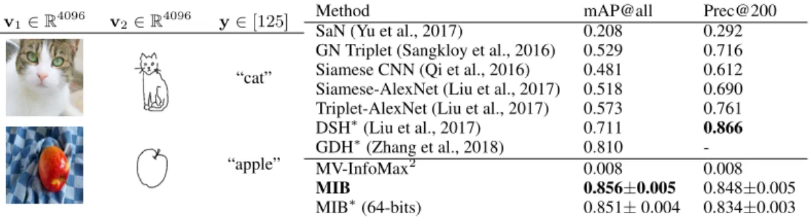
v1∈R4096 v2∈R4096 y∈[125]

“cat”

“apple”

Method mAP@all Prec@200

SaN (Yu et al., 2017) 0.208 0.292

GN Triplet (Sangkloy et al., 2016) 0.529 0.716

Siamese CNN (Qi et al., 2016) 0.481 0.612

Siamese-AlexNet (Liu et al., 2017) 0.518 0.690 Triplet-AlexNet (Liu et al., 2017) 0.573 0.761

DSH∗(Liu et al., 2017) 0.711 0.866

GDH∗(Zhang et al., 2018) 0.810

-MV-InfoMax2 0.008 0.008

MIB 0.856±0.005 0.848±0.005

MIB∗(64-bits) 0.851±0.004 0.834±0.003

Table 1: Examples of the two views and class label from the Sketchy dataset (on the left) and comparison between MIB and other popular models in literature on the sketch-based image retrieval task (on the right). ∗denotes models that use a 64-bits binary representation. The results for MIB corresponds toβ = 1.

and Achille & Soatto (2018). The direct removal of superfluous information has, so far, been done only in supervised settings (Alemi et al., 2017). Conversely, β-VAE models remove information indiscriminately without identifying which part is superfluous, and the InfoMax and Multi-View InfoMax methods do not explicitly try to remove superfluous information at all. In fact, among the representations that are optimal according to Multi-View InfoMax (purple dotted line in Figure 2), the MIB objective results in the representation with the least superfluous information, i.e. the most robust.

5

E

In this section we demonstrate the effectiveness of our model against state-of-the-art baselines in both the multi-view and single-view setting. In the single-view setting, we also estimate the coor-dinates on the Information Plane for each of the baseline methods as well as our method to validate the theory in Section 3.

The results reported in the following sections are obtained using the Jensen-ShannonIJ S (Devon Hjelm et al., 2019; Poole et al., 2019) estimator, which resulted in better performance for MIB and the other InfoMax-based models (Table 2 in the supplementary material). In order to facilitate the comparison between the effect of the different loss functions, the same estimator is used across the different models.

5.1 MULTI-VIEWTASKS

We compare MIB on the sketch-based image retrieval (Sangkloy et al., 2016) and Flickr multiclass image classification (Huiskes & Lew, 2008) tasks with domain specific and prior multi-view learning methods.

Sketchy The Sketchy dataset (Sangkloy et al., 2016) consists of 12,500 images and 75,471 hand-drawn sketches of objects from 125 classes. As in Liu et al. (2017), we also include another 60,502 images from the ImageNet (Deng et al., 2009) from the same classes, which results in total 73,002 natural object images. As per the experimental protocol of Zhang et al. (2018), a total of 6,250 sketches (50 sketches per category) are randomly selected and removed from the training set for test-ing purpose, which leaves 69,221 sketches for traintest-ing the model. The sketch-based image retrieval task is a ranking of 73,002 natural images according to the unseen test (query) sketch. Retrieval is done for our model by generating representations for the query sketch as well as all natural images, and ranking the image by the euclidean distance of their representation from the sketch represen-tation. The baselines use various domain specific ranking methodologies. Model performance is computed based on the class of the ranked pictures corresponding to the query. The training set consists of pairs of imagev1and sketchv2randomly selected from the same class, to ensure that

both views contain the equivalent label information (mutual redundancy).

Following recent prior works (Zhang et al., 2018; Dutta & Akata, 2019), we use features extracted from images and sketches by a VGG (Simonyan & Zisserman, 2014) architecture trained for

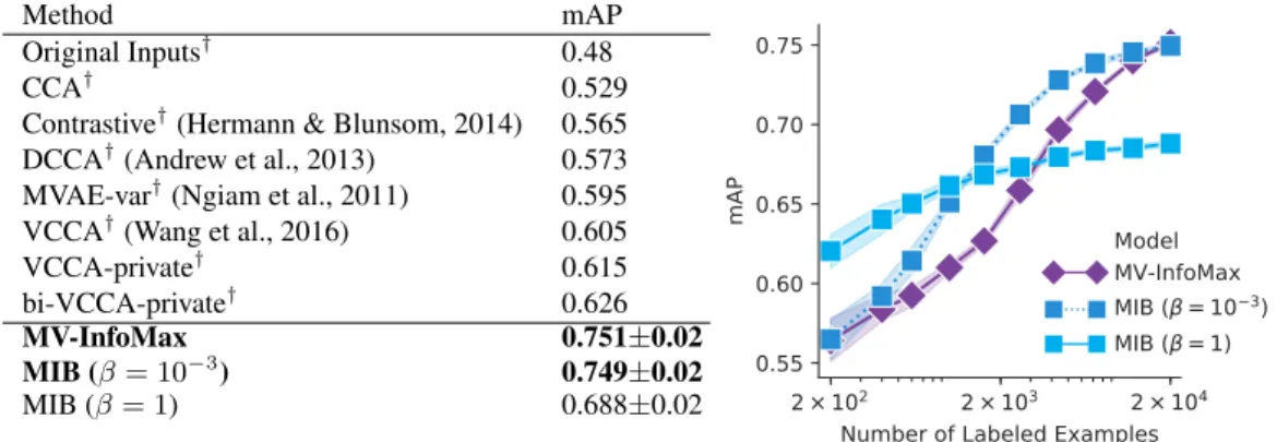
classi-Method mAP

Original Inputs† 0.48

CCA† 0.529

Contrastive†(Hermann & Blunsom, 2014) 0.565 DCCA†(Andrew et al., 2013) 0.573 MVAE-var†(Ngiam et al., 2011) 0.595

VCCA†(Wang et al., 2016) 0.605

VCCA-private† 0.615

bi-VCCA-private† 0.626

MV-InfoMax 0.751±0.02

MIB (β= 10−3_{) 0.749±0.02}

MIB (β= 1) 0.688±0.02

2 × 10

2 × 10

2 × 10

Number of Labeled Examples

0.55

0.60

0.65

0.70

0.75

mAP

Model

MV-InfoMax

MIB ( = 10

₎

MIB ( = 1)

Figure 3: Left: mean average precision (mAP) of the classifier trained on different multi-view representations for the MIR-Flickr task. Right: comparing the performance for different values of βand percentages of given labeled examples (from 1% up to 100%). Each model uses encoders of comparable size, producing a 1024d representation.†results from Wang et al. (2016).

fication on the TU-Berlin dataset (Eitz et al., 2012). The resulting flattened 4096-dimensional feature vectors are fed to our image and sketch encoders to produce a 64-dimensional representation. Both encoders consist of neural networks with hidden layers of 2048 and 1024 units respectively. Size of the representation and regularization strengthβ are tuned on a validation sub-split. We evaluate MIB on five different train/test splits1_{and report mean and standard deviation in Table 5.1. Further}

details on our training procedure and architecture are in Appendix G.

Table 5.1 shows that the our model achieves strong performance for both mean average precision (mAP@all) and precision at 200 (Prec@200), suggesting that the representation is able to capture the common class information between the paired pictures and sketches. The effectiveness of MIB on the retrieval task can be mostly imputed to the regularization introduced with the symmetrized KL divergence between the two encoded views. Other than discarding view-private information, this term actively aligns the representations ofv1andv2, making the MIB model especially suitable

for retrieval tasks

MIR-Flickr The MIR-Flickr dataset (Huiskes & Lew, 2008) consists of 1M images annotated with 800K distinct user tags. Each image is represented by a vector of 3,857 hand-crafted image features (v1), while the 2,000 most frequent tags are used to produce a 2000-dimensional

multi-hot encoding (v2) for each picture. The dataset is divided into labeled and unlabeled sets that

respectively contain 975K and 25K images, where the labeled set also contains 38 distinct topic classes together with the user tags.

Training images with less than two tags are removed, which reduces the total number of training samples to 749,647 pairs (Sohn et al., 2014; Wang et al., 2016). The labeled set contains 5 different splits of train, validation and test sets of size 10K/5K/10K respectively. Following a standard pro-cedure in literature (Srivastava & Salakhutdinov, 2014; Wang et al., 2016), we train our model on the unlabeled pairs of images and tags. Then a multi-label logistic classifier is trained from the rep-resentation of 10K labeled train images to the corresponding macro-categories. The quality of the representation is assessed based on the performance of the trained logistic classifier on the labeled test set. Each encoder consists of a multi-layer perceptron of 4 hidden layers with ReLU activations learning two 1024-dimensional representationsz1andz2 for imagesv1 and tagsv2 respectively.

Examples of the two views, labels, and further details on the training procedure are in Appendix G. Our MIB model is compared with other popular multi-view learning models in Figure 3 forβ = 0 (Multi-View InfoMax),β = 1andβ = 10−3_{(best on validation set). Although the tuned MIB}

per-forms similarly to Multi-View InfoMax with a large number of labels, it outperper-forms it when fewer

1_{Processed dataset and splits will be publicly released on paper acceptance} 2

These results are included only for completeness, as the Multi-View InfoMax objective does not produce consistent representations for the two views so there is no straight-forward way to use it for ranking.

0 2 4 6 8 10 12 14

I(

x;

z)

I(

z

;

y

)

0.3 0.4 0.5 0.6 0.7 0.8 0.9 1.0 Accuracy Model VAE ( = 0) VAE ( = 4) VAE ( = 8) InfoMax MV-InfoMax MIB ( = 1)

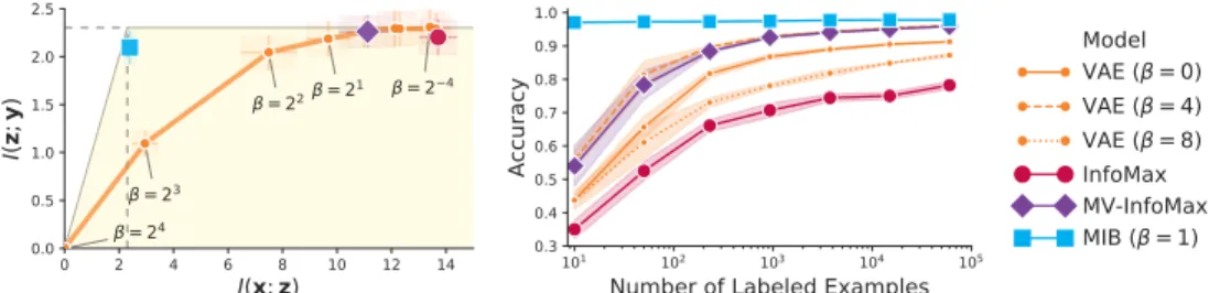
Figure 4: Comparing the representations obtained with different objectives on MNIST dataset. The empirical estimation of the coordinates on the Information Plane (in nats on the left) is followed by the respective classification accuracy for different number of randomly sampled labels (from 1 example per label up to 6000 examples per label). Representations that discard more observational information tend to perform better in scarce label regimes. The measurements used to produce the two graphs are reported in Appedix G.4.1.

labels are available. Furthermore, by choosing a largerβ the accuracy of our model drastically in-creases in scarce label regimes, while slightly reducing the accuracy when all the labels are observed (see right side of Figure 3). This effect is likely due to a violation of the mutual redundancy con-straint (see Figure 6 in the supplementary material) which can be compensated with smaller values ofβfor less aggressive compression.

A possible reason for the effectiveness of MIB against some of the other baselines may be our ability to use mutual information estimators that do not require reconstruction. Both Multi-View VAE (MVAE) and Deep Variational CCA (VCCA) rely on a reconstruction term to capture cross-modal information, which can introduce bias that decreases performance.

5.2 SELF-SUPERVISEDSINGLE-VIEWTASK

In this section, we compare the performance of different unsupervised learning models by measuring their data efficiency and empirically estimating the coordinates of their representation on the Infor-mation Plane. Since accurate estiInfor-mation of mutual inforInfor-mation is extremely expensive (McAllester & Stratos, 2018), we focus on relatively small experiments that aim to uncover the difference be-tween popular approaches for representation learning.

The dataset is generated from MNIST by creating the two views, v1 andv2, via the application

of data augmentation consisting of small affine transformations and independent pixel corruption to each image. These are kept small enough to ensure that label information is not effected. Each pair of views is generated from the same underlying image, so no label information is used in this process (details in Appendix G). To evaluate, we train the encoders using the unlabeled multi-view dataset just described, and then fix the representation model. A logistic regression model is trained using the resulting representations along with a subset of labels for the training set, and we report the accuracy of this model on a disjoint test set as is standard for the unsupervised representation learning literature (Tschannen et al., 2019; Tian et al., 2019; van den Oord et al., 2018). We estimate I(x;z)andI(y;z)using mutual information estimation networks trained from scratch on the final representations using batches of joint samples{(x(i),y(i),z(i))}B

i=1∼p(x,y)pθ(z|x). All models are trained using the same encoder architecture consisting of 2 layers of 1024 hidden units with ReLU activations, resulting in 64-dimensional representations. The same data augmentation proce-dure was also applied for single-view architectures and models were trained for 1 million iterations with batch sizeB = 64.

Figure 4 summarizes the results. The empirical measurements of mutual information reported on the Information Plane are consistent with the theoretical analysis reported in Section 4: models that retain less information about the data while maintaining the maximal amount of predictive infor-mation, result in better classification performance at low-label regimes, confirming the hypothesis that discarding irrelevant information yields robustness and more data-efficient representations. No-tably, the MIB model withβ= 1retains almost exclusively label information, hardly decreasing the classification performance when only one label is used for each data point.

6

C

F

In this work, we introduce Multi-View Information Bottleneck, a novel method that relies on mul-tiple data-views to produce robust representation for downstream tasks. Most of the multi-view literature operates under the assumption that each view is individually sufficient for determining the label (Zhao et al., 2017), while our method only requires the weaker mutual redundancy condition outlined in Section 3, enabling it to be applied to any traditional multi-view task. In our experi-ments, we compared MIB empirically against other approaches in the literature on three such tasks: sketch-based image retrieval, multi-view and unsupervised representation learning. The strong per-formance obtained in the different areas show that Multi-View Information Bottleneck can be practi-cally applied to various tasks for which the paired observations are either available or are artificially produced. Furthermore, the positive results on the MIR-Flickr dataset show that our model can work well in practice even when mutual redundancy holds only approximately.

There are multiple extensions that we would like to explore in future work. One interesting direction would be considering more than two views. In Appendix D we discuss why the mutual redundancy condition cannot be trivially extended to more than two views, but we still believe such an extension is possible. Secondly, we believe that exploring the role played by different choices of data aug-mentation could bridge the gap between the Information Bottleneck principle and with the literature on invariant neural networks (Bloem-Reddy & Whye Teh, 2019), which are able to exploit known symmetries and structure of the data to remove superfluous information.

ACKNOWLEDGMENTS

This work has received funding from the ERC under the Horizon 2020 program (grant agreement No. 853489). The Titan Xp and Titan V used for this research were donated by the NVIDIA Corporation.

R

Alessandro Achille and Stefano Soatto. Emergence of Invariance and Disentanglement in Deep Representations. JMLR, 2018.

Alexander A. Alemi, Ian Fischer, Joshua V. Dillon, and Kevin Murphy. Deep Variational Informa-tion Bottleneck. InICLR, 2017.

Alexander A. Alemi, Ben Poole, Ian Fischer, Joshua V. Dillon, Rif A. Saurous, and Kevin Murphy. Fixing a Broken ELBO. InICML, 2018.

Galen Andrew, Raman Arora, Jeff Bilmes, and Karen Livescu. Deep canonical correlation analysis. InICML, 2013.

Philip Bachman, R Devon Hjelm, and William Buchwalter. Learning Representations by Maximiz-ing Mutual Information Across Views.arXiv, 2019.

David Barber and Felix Agakov. The im algorithm: A variational approach to information maxi-mization. InNIPS, 2003.

Benjamin Bloem-Reddy and Yee Whye Teh. Probabilistic symmetry and invariant neural networks. arXiv, 2019.

Christopher P. Burgess, Irina Higgins, Arka Pal, Loic Matthey, Nick Watters, Guillaume Desjardins, and Alexander Lerchner. Understanding disentangling inβ-VAE.arXiv, 2018.

Xi Chen, Diederik P. Kingma, Tim Salimans, Yan Duan, Prafulla Dhariwal, John Schulman, Ilya Sutskever, and Pieter Abbeel. Variational Lossy Autoencoder. InICLR, 2017.

J. Deng, W. Dong, R. Socher, L. Li, Kai Li, and Li Fei-Fei. Imagenet: A large-scale hierarchical image database. InCVPR, 2009.

Jacob Devlin, Ming-Wei Chang, Kenton Lee, and Kristina Toutanova. Bert: Pre-training of deep bidirectional transformers for language understanding.arXiv, 2018.

R Devon Hjelm, Alex Fedorov, Samuel Lavoie-Marchildon, Karan Grewal, Phil Bachman, Adam Trischler, and Yoshua Bengio. Learning deep representations by mutual information estimation and maximization. InICLR, 2019.

Anjan Dutta and Zeynep Akata. Semantically tied paired cycle consistency for zero-shot sketch-based image retrieval. InCVPR, 2019.

Mathias Eitz, James Hays, and Marc Alexa. How do humans sketch objects? ACM TOG, 2012. Y. Gong, S. Lazebnik, A. Gordo, and F. Perronnin. Iterative quantization: A procrustean approach

to learning binary codes for large-scale image retrieval.TPAMI, 2013.

Ishaan Gulrajani, Kundan Kumar, Faruk Ahmed, Adrien Ali Taiga, Francesco Visin, David Vazquez, and Aaron Courville. PixelVAE: A Latent Variable Model for Natural Images. InICLR, 2017. Olivier J. H´enaff, Ali Razavi, Carl Doersch, S. M. Ali Eslami, and Aaron van den Oord.

Data-Efficient Image Recognition with Contrastive Predictive Coding.arXiv, 2019.

Karl Moritz Hermann and Phil Blunsom. Multilingual Distributed Representations without Word Alignment. InICLR, 2014.

Irina Higgins, Loic Matthey, Arka Pal, Christopher Burgess, Xavier Glorot, Matthew Botvinick, Shakir Mohamed, and Alexander Lerchner. beta-vae: Learning basic visual concepts with a constrained variational framework. InICLR, 2017.

Geoffrey Hinton, Li Deng, Dong Yu, George Dahl, Abdel-rahman Mohamed, Navdeep Jaitly, An-drew Senior, Vincent Vanhoucke, Patrick Nguyen, Brian Kingsbury, et al. Deep neural networks for acoustic modeling in speech recognition.SPM, 2012.

Mark J. Huiskes and Michael S. Lew. The mir flickr retrieval evaluation. InICMIR, pp. 39–43, 2008.

Mohamed Ishmael Belghazi, Aristide Baratin, Sai Rajeswar, Sherjil Ozair, Yoshua Bengio, Aaron Courville, and R Devon Hjelm. MINE: Mutual Information Neural Estimation. InICML, 2018. Xu Ji, Jo˜ao F. Henriques, and Andrea Vedaldi. Invariant Information Clustering for Unsupervised

Image Classification and Segmentation. InICCV, 2019.

Danilo Jimenez Rezende and Shakir Mohamed. Variational Inference with Normalizing Flows. In ICML, 2015.

Diederik P Kingma and Max Welling. Auto-Encoding Variational Bayes. InICLR, 2014.

Durk P Kingma, Tim Salimans, Rafal Jozefowicz, Xi Chen, Ilya Sutskever, and Max Welling. Im-proved variational inference with inverse autoregressive flow. InNIPS, 2016.

Yann LeCun, Yoshua Bengio, and Geoffrey Hinton. Deep learning. Nature, 2015. R. Linsker. Self-organization in a perceptual network. Computer, 1988.

Li Liu, Fumin Shen, Yuming Shen, Xianglong Liu, and Ling Shao. Deep Sketch Hashing: Fast Free-hand Sketch-Based Image Retrieval. InCVPR, 2017.

David McAllester and Karl Stratos. Formal Limitations on the Measurement of Mutual Information. arXiv, 2018.

Jiquan Ngiam, Aditya Khosla, Mingyu Kim, Juhan Nam, Honglak Lee, and Andrew Y. Ng. Multi-modal deep learning. InICML, 2011.

XuanLong Nguyen, Martin J. Wainwright, and Michael I. Jordan. Estimating divergence functionals and the likelihood ratio by convex risk minimization. InNIPS, 2008.

Ben Poole, Sherjil Ozair, Aaron van den Oord, Alexander A. Alemi, and George Tucker. On Varia-tional Bounds of Mutual Information. InICML, 2019.

Y. Qi, Y. Song, H. Zhang, and J. Liu. Sketch-based image retrieval via siamese convolutional neural network. InICIP, 2016.

Alec Radford, Jeffrey Wu, Rewon Child, David Luan, Dario Amodei, and Ilya Sutskever. Language models are unsupervised multitask learners.OpenAI Blog, 2019.

Patsorn Sangkloy, Nathan Burnell, Cusuh Ham, and James Hays. The sketchy database: learning to retrieve badly drawn bunnies.ACM TOG, 2016.

Karen Simonyan and Andrew Zisserman. Very Deep Convolutional Networks for Large-Scale Image Recognition.arXiv, 2014.

Kihyuk Sohn, Wenling Shang, and Honglak Lee. Improved multimodal deep learning with variation of information. InNIPS, 2014.

Nitish Srivastava and Ruslan Salakhutdinov. Multimodal learning with deep boltzmann machines. JMLR, 2014.

Wanhua Su, Yan Yuan, and Mu Zhu. A relationship between the average precision and the area under the roc curve. InICTIR, 2015.

Ilya Sutskever, Geoffrey E Hinton, and A Krizhevsky. Imagenet classification with deep convolu-tional neural networks. InNIPS, 2012.

Yonglong Tian, Dilip Krishnan, and Phillip Isola. Contrastive Multiview Coding.arXiv, 2019. Naftali Tishby and Noga Zaslavsky. Deep Learning and the Information Bottleneck Principle. In

ITW, 2015.

Naftali Tishby, Fernando C. Pereira, and William Bialek. The information bottleneck method.arXiv, 2000.

Jakub M. Tomczak and Max Welling. VAE with a VampPrior. InAISTATS, 2018.

Michael Tschannen, Josip Djolonga, Paul K. Rubenstein, Sylvain Gelly, and Mario Lucic. On Mutual Information Maximization for Representation Learning.arXiv, 2019.

Aaron van den Oord, Yazhe Li, and Oriol Vinyals. Representation Learning with Contrastive Pre-dictive Coding.arXiv, 2018.

Weiran Wang, Xinchen Yan, Honglak Lee, and Karen Livescu. Deep Variational Canonical Corre-lation Analysis.arXiv, 2016.

Qian Yu, Yongxin Yang, Yi-Zhe Song, Tao Xiang, and Timothy Hospedales. Sketch-a-Net that Beats Humans.IJCV, 2017.

Jingyi Zhang, Fumin Shen, Li Liu, Fan Zhu, Mengyang Yu, Ling Shao, Heng Tao Shen, and Luc Van Gool. Generative domain-migration hashing for sketch-to-image retrieval. InECCV, 2018. Jing Zhao, Xijiong Xie, Xin Xu, and Shiliang Sun. Multi-view learning overview: Recent progress

A

P

M

I

E

In this section we enumerate some of the properties of mutual information that are used to prove the theorems reported in this work. For any random variablesw,x,yandz:

(P1) Positivity:

I(x;y)≥0, I(x;y|z)≥0 (P2) Chain rule:

I(xy;z) =I(y;z) +I(x;z|y) (P3) Chain rule (Multivariate Mutual Information):

I(x;y;z) =I(y;z)−I(y;z|x) (P4) Positivity of discrete entropy:

For discretex

H(x)≥0, H(x|y)≥0 (P5) Entropy and Mutual Information

H(x) =H(x|y) +I(x;y)

B

T

P

Proposition B.1. Let x and y be random variables with joint distribution p(x,y). Letz be a representation ofx, thenzis sufficient foryif and only ifI(x;y) =I(y;z)

Hypothesis:

(H1) I(y;z|x) = 0

Thesis:

(T1) I(x;y|z) = 0 ⇐⇒ I(x;y) =I(y;z)

Proof.

I(x;y|z)(P=3)I(x;y)−I(x;y;z)(P=3)I(x;y)−I(y;z)−I(y;z|x)

(H1)

= I(x;y)−I(y;z)

Since bothI(x;y)andI(y;z)are non-negative(P1),I(x;y|z) = 0 ⇐⇒ I(y;z) =I(x;y)

B.2 NOFREEGENERALIZATION

Theorem B.1. Letx,zandybe random variables with joint distributionp(x,y,z). Letz0 be a representation ofxthat satisfiesI(x;z)> I(x;z0_{), then it is always possible to find a labelyfor}

whichz0is not predictive forywhilezis.

Hypothesis:

(H1) I(y;z0|x) = 0

(T1) I(x;z0)< I(x;z) =⇒ ∃y.I(y;z)> I(y;z0) = 0

Proof. By construction.

1. We first factorizex as a function of two independent random variables (Proposition 2.1 Achille & Soatto (2018)) by pickingysuch that:

(C1) I(y;z0) = 0

(C2) x=f(z0,y)

for some deterministic functionf. Note that suchyalways exists. 2. Sincexis a function ofyandz0:

(C4) I(x;z|yz0) = 0

ConsideringI(y;z):

I(y;z)(P=3)I(y;z|x) +I(x;y;z)

(P1)

≥ I(x;y;z)

(P3)

= I(x;z)−I(x;z|y)

(P3)

= I(x;z)−I(x;z|yz0)−I(x;z;z0|y)

(C2)

= I(x;z)−I(x;z;z0|y)

(P3)

= I(x;z)−I(x;z0|y) +I(x;z0|yz)

(P1)

≥ I(x;z)−I(x;z0|y)

(P3)

= I(x;z)−I(x;z0) +I(x;y;z0)

(P3)

= I(x;z)−I(x;z0) +I(y;z0)−I(y;z0|x)

(P1)

≥ I(x;z)−I(x;z0)−I(y;z0|x)

(H1)

= I(x;z)−I(x;z0)

WheneverI(x;z)> I(x;z0),I(y;z)must be strictly positive, whileI(y;z0) = 0by construction. Therefore suchyexists.

Corollary B.1.1. Letz0be a representation ofxthat discards observational information. There is always a labelyfor which az0is not predictive, while the original observations are.

Hypothesis:

(H1) xis discrete (empirical distribution)

(H2) I(z0;x)< H(x)

Thesis:

(T1) ∃y.I(y;x)> I(y;z0) = 0

Proof. By construction using Theorem B.1. 1. Setz=x:

(C1) I(x;z) (P5)

2. I(z0;x)< H(x) (=C⇒1) I(z0;x)< I(x;z)

Since the hypothesis are met, we conclude that there existysuch thatI(y;x)> I(y;z0) = 0 B.3 MULTI-VIEW

B.3.1 MULTI-VIEWREDUNDANCY ANDSUFFICIENCY

Proposition B.2. Letv1,v2,ybe random variables with joint distributionp(v1,v2,y). Letz1be

a representation ofv1, then:

I(v1;y|z1)≤I(v1;v2|z1) +I(v1;y|v2)

Hypothesis:

(H1) I(y;z1|v2v1) = 0

Thesis:

(T1) I(v1;y|z1)≤I(v1;v2|z1) +I(v1;y|v2)

Proof. Sincez1is a representation ofv1:

(C1) I(y;z1|v2v1) = 0 Therefore: I(v1;y|z1) (P3) = I(v1;y|z1v2) +I(v1;v2;y|z1) (P3)

= I(v1;y|v2)−I(v1;y;z1|v2) +I(v1;v2;y|z1) (P3)

= I(v1;y|v2)−I(y;z1|v2) +I(y;z1|v2v1) +I(v1;v2;y|z1) (P1)

≤ I(v1;y|v2) +I(y;z1|v2v1) +I(v1;v2;y|z1) (H1)

= I(v1;y|v2) +I(v1;v2;y|z1) (P3)

= I(v1;y|v2) +I(v1;v2|z1)−I(v1;v2|z1y) (P1)

≤ I(v1;y|v2) +I(v1;v2|z1)

Proposition B.3. Letv1be a redundant view with respect tov2fory. Any representationz1ofv1

that is sufficient forv2is also sufficient fory.

Hypothesis:

(H1) I(y;z1|v2v1) = 0

(H2) I(y;v1|v2) = 0

Thesis:

(T1) I(v1;v2|z1) = 0 =⇒ I(v1;y|z1) = 0

Proof. Using the results from Theorem B.2: I(v1;y|z1)

(T hB.2)

≤ I(v1;y|v2) +I(v1;v2|z1) (H2)

= I(v1;v2|z1)

Theorem B.2. Letv1,v2 and ybe random variables with distributionp(v1,v2,y). Letzbe a

representation ofv1, then

I(y;z1)≥I(y;v1v2)−I(v1;v2|z1)−I(v1;y|v2)−I(v2;y|v1)

Hypothesis:

(H1) I(y;z1|v1v2) = 0

Thesis:

(T1) I(y;z1)≥I(y;v1v2)−I(v1;v2|z1)−I(v1;y|v2)−I(v2;y|v1)

Proof. I(y;z1) (P3) = I(y;z1|v1v2) +I(y;v1v2;z1) (H1) = I(y;v1v2;z1) (P3) = I(y;v1v2)−I(y;v1v2|z1) (P2)

= I(y;v1v2)−I(y;v1|z1)−I(y;v2|z1v1) (P3)

= I(y;v1v2)−I(y;v1|z1)−I(y;v2|v1) +I(y;v2;z1|v1) (P3)

= I(y;v1v2)−I(y;v1|z1)−I(y;v2|v1) +I(y;z1|v1)−I(y;z1|v1v2) (H1)

= I(y;v1v2)−I(y;v1|z1)−I(y;v2|v1) +I(y;z1|v1) (P1)

≥ I(y;v1v2)−I(y;v1|z1)−I(y;v2|v1) (P ropB.2)

≥ I(y;v1v2)−I(v1;y|v2)−I(v1;v2|z1)−I(y;v2|v1)

Corollary B.2.1. Letv1andv2be mutually redundant views fory. Letz1be a representation of

v1that is sufficient forv2. Then:

I(y;z1) =I(v1v2;y) Hypothesis: (H1) I(y;z1|v1v2) = 0 (H2) I(y;v1|v2) +I(y;v2|v1) = 0 (H3) I(v2;v1|z) = 0 Thesis: (T1) I(y;z1) =I(v1v2;y)

Proof. Using Theorem B.2 I(y;z1)

(T hB.2)

≥ I(y;v1v2)−I(v1;y|v2)−I(v1;v2|z1)−I(y;v2|v1) (H2)

= I(y;v1v2)−I(v1;v2|z1) (H3)

= I(y;v1v2)

SinceI(y;z1) ≤I(y;v1v2)is a consequence of the data processing inequality, we conclude that

B.4 SUFFICIENCY ANDAUGMENTATION

Letxandybe random variables with domainXandYrespectively. LetTbe a class of functions

t:X→Wand lett1andt2be a random variables overTthat depends only onx. For the theorems

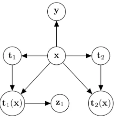
and corollaries discussed in this section, we are going to consider the independence assumption that can be derived from the graphical modelGreported in Figure 5.

x

t1 t2

y

t1(x) z1 t2(x)

Figure 5: Visualization of the graphical modelGthat relates the observationsx, labely, functions used for augmentationt1,t2and the representationz1.

Proposition B.4. WheneverI(t1(x);y) =I(t2(x);y) =I(x;y)the two viewst1(x)andt2(x)

must be mutually redundant fory. Hypothesis:

(H1) Independence relations determined byG

Thesis:

(T1) I(t1(x);y) =I(t2(x);y) =I(x;y) =⇒ I(t1(x);y|t2(x)) +I(t2(x);y|t1(x)) = 0

Proof.

1. ConsideringGwe have: (C1) I(t1(x);y|xt2(x)) = 0

(C2) I(y;t2(x)|x) = 0

2. Sincet2(x)is uniquely determined byxandt2:

3. ConsiderI(t1(x);y|t2(x)) I(t1(x);y|t2(x)) (P3) = I(t1(x);y|xt2(x)) +I(t1(x);y;x|t2(x)) (C1) = I(t1(x);y;x|t2(x)) (P3) = I(y;x|t2(x))−I(y;x|t1(x)t2(x)) (P1) ≤ I(y;x|t2(x)) (P3) = I(y;x)−I(y;x;t2(x)) (P3)

= I(y;x)−I(y;t2(x)) +I(y;t2(x)|x) (P3)

= I(y;x)−I(y;t2(x)) +I(y;t2(x)|t2x) +I(y;t2(x);t2|x) (C3)

= I(y;x)−I(y;t2(x)) +I(y;t2(x);t2|x) (P3)

= I(y;x)−I(y;t2(x)) +I(y;t2(x)|x)−I(y;t2(x)|t2x) (P1)

≥ I(y;x)−I(y;t2(x)) +I(y;t2(x)|x) (C2)

≥ I(y;x)−I(y;t2(x))

ThereforeI(y;x) =I(y;t2(x)) =⇒ I(t1(x);y|t2(x)) = 0

The proof forI(y;x) = I(y;t1(x)) =⇒ I(t2(x);y|t1(x)) = 0 is symmetric, therefore we

concludeI(t1(x);y) = I(t2(x);y) = I(x;y) =⇒ I(t1(x);y|t2(x)) +I(t2(x);y|t1(x)) =

0

Theorem B.3. LetI(t1(x);y) =I(t2(x);y) =I(x;y). Letz1be a representation oft1(x). If

z1is sufficient fort2(x)thenI(x;y) =I(y;z1).

Hypothesis:

(H1) Independence relations determined byG

(H2) I(t1(x);y) =I(t2(x);y) =I(x;y)

Thesis:

(T1) I(t1(x);t2(x)|z1) = 0 =⇒ I(x;y) =I(y;z1)

Proof. Sincet1(x)is redundant fort2(x)(Proposition B.4) any representationz1oft1(x)that is

sufficient fort2(x)must also be sufficient fory(Theorem B.2). Using Proposition B.1 we have

I(y;z1) = I(y;t1(x)). SinceI(y;t1(x)) = I(y;x) by hypothesis, we conclude I(x;y) =

I(y;z1)

C

I

P

Every representationzofxmust satisfy the following constraints:

• 0≤I(y;z)≤I(x;y): The amount of label information ranges from 0 to the total predic-tive information accessible from the raw observationsI(x;y).

• I(y;z)≤I(x;z)≤I(y;z) +H(x|y): The representation must contain more information about the observations than about the label. Whenxis discrete, the amount of discarded label informationI(x;y)−I(y;z)must be smaller than the amount of discarded observa-tional informationH(x)−I(x;z), which impliesI(x;z)≤I(y;z) +H(x|y).

Proof. Sincezis a representation ofx: (C1) I(y;z|x) = 0

Considering the four bounds separately: 1. I(y;z)≥0: Follows fromP1

2. I(x;z)≥I(y;z): Follows from(T1)in Lemma B.1

3. I(y;z)≤I(y;x): Data processing inequality

I(y;z)(P=3)I(y;z|x) +I(y;z;x)

(C1) = I(y;z;x) (P3) = I(x;y)−I(x;y|z) (P1) ≤ I(x;y) 4. I(x;z)≤I(y;z) +H(x|y):

I(x;z)(P=3)I(x;z|y) +I(x;y;z)

(P3)

= I(x;z|y) +I(y;z)−I(y;z|x)

(C1)

= I(x;z|y) +I(y;z)

(H2+P4)

≤ I(x;z|y) +H(x|yz) +I(y;z)

(P5)

= H(x|y) +I(y;z)

Note that(H2)is needed only to prove bound4. For continuousxbounds1,2and3still hold.

D

N

-

M

R

The mutual redundancy condition between two viewsv1andv2for a labelycan not be trivially

ex-tended to an arbitrary number of views, as the relation is not transitive because of some higher order interaction between the different views and the label. This can be shown with a simple example. Given three viewsv1,v2andv3and a taskysuch that:

• v1andv2are mutually redundant fory

• v2andv3are mutually redundant fory

Then,v1is not necessarily mutually redundant with respect tov3fory.

We can show this with a simple example, Letv1,v2andv3be fair and independent binary random

variables. Definingyas the exclusive or ofv1andv3(y:=v1XORv3), we have thatI(v1;y) =

I(v3;y) = 0. In this settings,v1andv2are mutually redundant fory:

I(v1;y|v2) =H(v1|v2)−H(v1|v2y) =H(v1)−H(v1) = 0

I(v2;y|v1) =H(v2|v1)−H(v2|v1y) =H(v2)−H(v2) = 0

Analogously, v2 andv3 are also mutually redundant for yas the three random variables are not

predictive for each other. Nevertheless,v1andv3and not mutually redundant fory:

I(v1;y|v3) =H(v1|v3)−H(v1|v3y) | {z } 0 =H(v1) = 1 I(v3;y|v1) =H(v3|v1)−H(v3|v1y) | {z } 0 =H(v3) = 1

WhereH(v1|v3y) = H(v3|v1y) = 0follows fromv1=v3XORyandv3=v1XORy, while

H(v1) =H(v3) = 1holds by construction.

This counter-intuitive higher order interaction between multiple views makes our theory non-trivial to generalize to more than two views, requiring an extension of our theory to ensure sufficiency for the label.

E

E

Different objectives in literature can be seen as a special case of the Multi-View Information Bot-tleneck principle. In this section we show that the supervised version of Information BotBot-tleneck is equivalent to the corresponding Multi-View version whenever the two redundant views have only label information in common. A second subsection show equivalence between InfoMax and Multi-View Information Bottleneck whenever the two views are identical.

E.1 MULTI-VIEWINFORMATIONBOTTLENECK ANDSUPERVISEDINFORMATION BOTTLENECK

Whenever the two mutually redundant viewsv1andv2have only label information in common (or

when one of the two views is the label itself) the Multi-View Information Bottleneck objective is equivalent to the respective supervised version. This can be shown by proving thatI(v1;z1|v2) =

I(v1;z1|y), i.e. a representationz1ofv1that is sufficient and minimal forv2is also sufficient and

minimal fory.

Proposition E.1. Letv1and v2be mutually redundant views for a label ythat share only label

information. Then a sufficient representationz1ofv1forv2that is minimal forv2is also a minimal

representation fory. Hypothesis: (H1) I(v1;y|v2) +I(v2;y|v1) = 0 (H2) I(v1;v2) =I(v1;vy) (H3) I(v1;v2|z1) = 0 Thesis: (T1) I(v1;z1|v2) =I(v1;z1|y) Proof. 1. ConsiderI(v1;z): I(v1;z1) (P3) = I(v1;z1|v2) +I(v1;v2;z1) (P3)

= I(v1;z1|v2) +I(v1;v2)−I(v1;v2|z1) (H3)

= I(v1;z1|v2) +I(v1;v2) (H1)

= I(v1;z1|v2) +I(v1;y)

3. I(v1;z)can be alternatively expressed as:

I(v1;z1) (P3)

= I(v1;z1|y) +I(v1;y;z1) (P3)

= I(v1;z1|y) +I(v1;y)−I(v1;y|z1) (Cor1)

= I(v1;z1|y) +I(v1;y)

Equating 1 and 3, we concludeI(v1;z1|v2) =I(v1;z1|y).

E.2 MULTI-VIEWINFORMATIONBOTTLENECK ANDINFOMAX

Wheneverv1 =v2, a representationz1ofv1that is sufficient forv1must contain all the original

information. Furthermore sinceI(v1;z1|v1) = 0for every representation, no superfluous

informa-tion can be identified and removed. As a consequence, a minimal sufficient representainforma-tionz1ofv1

forv1is any representation for which mutual information is maximal, hence InfoMax.

F

L

C

Starting from Equation 3, we consider the sum of the lossesL1(θ;λ1)andL2(ψ;λ2)that aim to

create the minimal sufficient representationsz1andz2respectively:

L1+2(θ, ψ;λ1, λ2) = (Iθ(v1;z1|v2) +Iψ(v2;z2|v1)) + (λ1Iθ(v1;v2|z1) +λ2Iψ(v1;v2|z1))

(6) Consideringz1andz2on the same domainZ,Iθ(v1;z1|v2)can be expressed as:

Iθ(v1;z1|v2) =Ev1,v2∼p(v1,v2)Ez∼pθ(z1|v1) logpθ(z1=z|v1=v1) pθ(z1=z|v2=v2) =Ev1,v2∼p(v1,v2)Ez∼pθ(z1|v1) logpθ(z1=z|v1=v1) pψ(z2=z|v2=v2) pψ(z2=z|v2=v2) pθ(z1=z|v2=v2) =DKL(pθ(z1|v1)||pψ(z2|v2))−DKL(pθ(z2|v1)||pψ(z2|v2)) ≤DKL(pθ(z1|v1)||pψ(z2|v2))

Note that the bound is tight whenever pψ(z2|v2)coincides withpθ(z1|v2). This happens

when-ever z1 andz2 produce a consistent encoding. Analogously Iψ(v2;z2|v1)is upper bounded by

DKL(pψ(z2|v2)||pθ(z1|v1)).

Iθ(v1;v2|z1)can be rephrased as:

Iθ(v1;v2|z1) =I(v1;v2)−Iθ(z1;v2) (P2) = I(v1;v2)−Iθ(z1;z2v2)−Iθ(z1;z2|v2) =∗I(v1;v2)−Iθ(z1;z2v2) =I(v1;v2)−Iθ(z1;z2)−Iθψ(z1;v2|z2) ≤I(v1;v2)−Iθψ(z1;z2)

Where∗follows fromz2representation ofv2. The bound reported in this equation is tight whenever

z2is sufficient forz1. This happens wheneverz2 contains all the information regardingz1(and

thereforev1). Once again, the same bound can symmetrically be used to defineIθ(v1;v2|z2) ≤

I(v1;v2)−Iθψ(z1;z2).

SinceI(v1;v2)is constant inθandψ, the loss function in Equation 6 can be upper-bounded with;

L1+2(θ, ψ;λ1, λ2)≤2DSKL(pθ(z1|v1)||pψ(z2|v2))−(λ1+λ2)Iθψ(z1;z2) (7) Where: DSKL(pθ(z1|v1)||pψ(z2|v2)) := 1 2DKL(pθ(z1|v1)||pψ(z2|v2)) + 1 2DKL(pψ(z2|v2)||pθ(z1|v1)) Lastly, multiplying both terms withβ:= 2

λ1+λ2 and re-parametrizing the objective, we obtain:

G

E

The two stochastic encoders pθ(z1|v1) and pψ(z2|v2) are modeled by Normal distributions

parametrized with neural networks(µθ,σ2θ)and(µψ,σψ2)respectively: pθ(z1|v1) :=N z1|µθ(v1),σθ2(v1)

pψ(z2|v2) :=N z2|µψ(v2),σ2ψ(v2)

Since the density of the two encoders can be evaluated, the symmetrized KL-divergence in equa-tion 4 can be directly computed. On the other hand,Iθψ(z1;z2)requires the use of a mutual

infor-mation estimator.

To facilitate the optimization, the hyper-parameterβ is slowly increased during training, starting from a small value ≈ 10−4 _{to its final value with an exponential schedule. This is because the}

mutual information estimator is trained together with the other architectures and, since it starts from a random initialization, it requires an initial warm-up. Starting with biggerβ results in the encoder collapsing into a fixed representation. The update policy for the hyper-parameter during training has not shown strong influence on the representation, as long as the mutual information estimator network has reached full capacity.

All the experiments have been performed using the Adam optimizer with a learning rate of10−4

for both encoders and the estimation network. Higher learning rate can result in instabilities in the training procedure. The results reported in the main text relied on the Jensen-Shannon mutual information estimator (Devon Hjelm et al., 2019) since the InfoNCE counterpart (van den Oord et al., 2018) generally resulted in worse performance that could be explained by the effect of the factorization of the critic network (Poole et al., 2019).

G.2 SKETCHYEXPERIMENTS

• Input:The two views for the sketch-based classification task consist of 4096 dimensional sketch and image features extracted from two distinct VGG-16 network models which were pre-trained on images and sketches from the TU-Berlin dataset Eitz et al. (2012) for end-to-end classification. The feature extractors are frozen during the training procedure of for the two representations. Each training iteration used batches of sizeB= 128.

• Encoder and Critic architectures:Both sketch and image encoders consist of multi-layer perceptrons of 2 hidden ReLU units of size 2,048 and 1,024 respectively with an output of size 2x64 that parametrizes mean and variance for the two Gaussian posteriors. The critic architecture also consists of a multi layer perceptron of 2 hidden ReLU units of size 512.

• βupdate policy: The initial value ofβis set to10−4_{. Starting from the 10,000}th_training

iteration, the value ofβis exponentially increased up to 1.0 during the following 250,000 training iterations. The value ofβ is then kept fixed to one until the end of the training procedure (500,000 iterations).

• Evaluation:All natural images are used as both training sets and retrieval galleries. The 64 dimensional real outputs of sketch and image representation are compared using Eu-clidean distance. For having a fair comparison other methods that rely on binary hashing (Liu et al., 2017; Zhang et al., 2018), we used Hamming distance on a binarized represen-tation (obtained by applying iterative quantization Gong et al. (2013) on our real valued representation). We report the mean average precision (mAP@all) and precision at top-rank 200 (Prec@200) Su et al. (2015) on both the real and binary representation to evaluate our method and compare it with prior works.

G.3 MIR-FLICKREXPERIMENTS

• Input:Whitening is applied to the handcrafted image features. Batches of sizeB = 128 are used for each update step.

• Encoders and Critic architectures:The two encoders consists of a multi layer perceptron of 4 hidden ReLU units of size 1,024, which exactly resemble the architecture used in

Figure 6: Examples of picturesv1, tagsv2and category labelsyfor the MIR-Flickr dataset

(Srivas-tava & Salakhutdinov, 2014). As visualized is the second row, the tags are not always predictive of the label. For this reason, the mutual redundancy assumption holds only approximately.

v1∈R3857 v2∈ {0,1} 2000 y∈ {0,1}38 “watermelon”, “hilarious”, “chihuahua”, “dog” “animals”, “dog”, “food” “colors”, “cores”, “centro”, “comercial”, “building” “clouds”, “sky”, “structures”

Wang et al. (2016). Both representationsz1 andz2 have a size of 1,024, therefore the

two architecture output a total of 2x1,024 parameters that define mean and variance of the respective factorized Gaussian posterior. Similarly to the Sketchy experiments, the critic is consists of a multi-layer perceptron of 2 hidden ReLU units of size 512.

• βupdate policy:The initial value ofβis set to10−8_{. Starting from 150000}th_{iteration,βis}

set to exponentially increase up to 1.0 (and10−3) during the following 150,000 iterations.

• Evaluation: Once the models are trained on the unlabeledset, the representation of the 25,000labeledimages is computed. The resulting vectors are used for training and eval-uating a multi-label logistic regression classifier on the respective splits. The optimal pa-rameters (such asβ) for our model are chosen based on the performance on the validation set. In Table 3, we report the aggregated mean of the 5 test splits as the final value mean average precision value.

G.4 MNIST EXPERIMENTS

• Input:The two viewsv1 andv2for the MNIST dataset are generated by applying small

translation ([0-10]%), rotation ([-15,15] degrees), scale ([90,110]%), shear ([-15,15] de-grees) and pixel corruption (20%). Batches of sizeB = 64samples are used during train-ing.

• Encoders, Decoders and Critic architectures: All the encoders used for the MNIST experiments consist of neural networks with two hidden layers of 1,024 units and ReLU activations, producing a 2x64-dimensional parameter vector that is used to parameterize mean and variance for the Gaussian posteriors. The decoders used for the VAE experiments also consist of the networks of the same size. Similarly, the critic architecture used for mutual information estimation consists of two hidden layers of 1,204 units each and ReLU activations.

• βupdate policy:The initial value ofβis set to10−3_{, which is increased with an}

exponen-tial schedule starting from the 50,000th_{until 1the 50,000}th_{iteration. The value ofβis then}

kept constant until the 1,000,000thiteration. The same annealing policy is used to trained the differentβ-VAEs reported in this work.

• Evaluation: The trained representation are evaluated following the well-known protocol described in Tschannen et al. (2019); Tian et al. (2019); Bachman et al. (2019); van den Oord et al. (2018). Each logistic regression is trained 5 different balanced splits of the training set for different percentages of training examples, ranging from 1 example per la-bel to the whole training set. The accuracy reported in this work has been computed on the disjoint test set. Mean and standard deviation are computed according to the 5 different subsets used for training the logistic regression. Mean and variance for the mutual informa-tion estimainforma-tion reported on the Informainforma-tion Plane (Figure 4) are computed by training two estimation networks from scratch on the final representation of the non-augmented train set. The two estimation architectures consist of 2 hidden layers of 2048 and 1024 units each, and have been trained with batches of sizeB = 256 for a total of approximately

25,000 iterations. The Jensen-Shannon mutual information lower bound is maximized dur-ing traindur-ing, while the numerical estimation are computed usdur-ing an energy-based bound (Poole et al., 2019; Devon Hjelm et al., 2019). The final values forI(x;z)andI(y;z)are computed by averaging the mutual information estimation on the whole dataset. In order to reduce the variance of the estimator, the lowest and highest 5% are removed before av-eraging. This practical detail makes the estimation more consistent and less susceptible to numerical instabilities.

G.4.1 RESULTS ANDVISUALIZATION

In this section we include additional quantitative results and visualizations which refer to the single-view MNIST experiments reported in section 5.2.

Table 2 reports the quantitative results used for to produce the visualizations reported in Figure 4, including the comparison between the performance resulting from different mutual information esti-mators. As the Jensen-Shannon estimator generally resulted in better performance for the InfoMax, MV-InfoMax and MIB models, all the experiments reported on the main text make use of this esti-mator. Note that the InfoMax model with theIJSestimator is equivalent to the global model reported

in Devon Hjelm et al. (2019), while MV-InfoMax with theINCEestimator results in a similar

archi-tecture to the one introduced in Tian et al. (2019).

Model I(x;z)[nats] I(z;y)[nats] Test Accuracy[%]

10 Ex 50 Ex 3750 Ex 60000 Ex VAE (beta=0) 12.5±0.7 2.3±0.2 43.8±1.6 65.6±3.3 89.0±0.4 91.3±0.1 VAE (beta=4) 7.5±1.0 2.0±0.2 55.9±2.6 81.4±4.0 94.2±0.3 96.0±0.2 VAE (beta=8) 3.0±0.5 1.0±0.1 43.8±2.8 61.1±4.8 81.9±1.1 87.2±0.6 InfoMax (INCE) 12.8±0.5 2.3±0.2 25.4±1.9 39.6±3.3 69.2±0.7 74.6±0.6 InfoMax (IJS) 13.7±0.7 2.2±0.2 35.0±2.8 52.5±2.8 74.4±1.1 78.2±1.2 MV-InfoMax (INCE) 12.2±0.7 2.3±0.2 50.2±3.6 75.8±3.8 94.6±0.4 96.5±0.1 MV-InfoMax (IJS) 11.1±1.0 2.3±0.2 54.0±6.1 78.3±4.4 94.1±0.3 95.90±0.08 MIB (β= 1, INCE) 4.6±0.7 2.1±0.2 81.8±5.0 92.7±0.9 97.19±0.08 97.75±0.05 MIB (β= 1, IJS) 2.4±0.2 2.1±0.2 97.1±0.2 97.2±0.2 97.70±0.06 97.82±0.01

Table 2: Comparison of the amount of input informationI(x;z), label information I(z;y), and accuracy of a linear classifier trained with different amount of labeled Examples (Ex) for the models reported in Figure 4. Both the results obtained using the Jensen-ShannonIJSD(Devon Hjelm et al.,

2019; Poole et al., 2019) and the InfoNCEINCE(van den Oord et al., 2018) estimators are reported.

Figure 7 reports the linear projection of the embedding obtained using the MIB model. The latent space appears to roughly consists of ten clusters which corresponds to the different digits. This observation is consistent with the empirical measurement of input and label informationI(x;z)≈

I(z;y)≈log 10, and the performance of the linear classifier in scarce label regimes. As the cluster are distinct and concentrated around the respective centroids, 10 labeled examples are sufficient to align the centroid coordinates with the digit labels.

H

A

H.1 DIFFERENT RANGES OF DATA AUGMENTATION

Figure 8 visualizes the effect of different ranges of corruption probabily as data augmentation strat-egy to produce the two viewsv1andv2. The MV-InfoMax Model does not seem to get any

ad-vantage from the use increasing amount of corruption, and it representation remains approximately in the same region of the information plane. On the other hand, the models trained with the MIB objective are able to take advantage of the augmentation to remove irrelevant data information and the representation transitions from the top right corner of the Information Plane (no-augmentation) to the top-left. When the amount of corruption approaches 100%, the mutual redundancy assump-tion is clearly violated, and the performances of MIB deteriorate. In the initial part of the transi-tions between the two regimes (which corresponds to extremely low probability of corruption) the MIB models drops some label information that is quickly re-gained when pixel corruption becomes

Figure 7: Linear projection of the embedding obtained by applying the MIB encoder to the MNIST test set. The 64 dimensional representation is projected onto the two principal components. Different colors are used to represent the 10 digit classes.

more frequent. We hypothesize that this behavior is due to a problem with the optimization proce-dure, since the corruption are extremely unlikely, the Monte-Carlo estimation for the symmetrized Kullback-Leibler divergence is more biased. Using more examples of views produced from the same data-point within the same batch could mitigate this issue.

0.0 2.5 5.0 7.5 10.0 12.5 15.0

I(

x

;

z

)

I(

z

;

y

)

Examples per Label 1

5 23 6000

Figure 8: Visualization of the coordinates on the Information Plane (plot on the left) and predic-tion accuracy (center and right) for the MV-InfoMax and MIB objectives with different amount of training labels and corruption percentage used for data-augmentation.

H.2 EFFECT OFβ

The hyper-parameterβ(Equation 5) determines the trade-off between sufficiency and minimality of the representation for the second data view. Whenβis zero, the training objective of MIB is equiv-alent to the Multi-View InfoMax target, since the representation has no incentive to discard any information. When0< β ≤1the sufficiency constrain is enforced, while the superfluous informa-tion is gradually removed from the representainforma-tion. Values ofβ >1can result in representations that violate the sufficiency constraint, since the minimization ofI(x;z|v2)is prioritized. The trade-off

resulting from the choice of differentβis visualized in Figure 9 and compared againstβ-VAE. Note that in each point of the pareto-front the MIB model results in a better trade-off betweenI(x;z) andI(y;z)when compared toβ-VAE. The effectiveness of the Multi-View Information Bottleneck model is also justified by the corresponding values of predictive accuracy.

0.0 2.5 5.0 7.5 10.0 12.5 15.0

I(

x

;

z

)

I(

z

;

y

)

Figure 9: Visualization of the coordinates on the Information Plane (plot on the left) and predic-tion accuracy (center and right) for theβ-VAE, Multi-View InfoMax and Multi-View Information Bottleneck objectives with different amount of training labels and different values of the respective hyperparameterβ.