Statistical clustering of data

(1)

Copyright by Lihao Zhang

(2)

The Report Committee for Lihao Zhang

Certifies that this is the approved version of the following report:

Statistical Clustering of Data

APPROVED BY

SUPERVISING COMMITTEE:

Thomas W. Sager, Supervisor Matthew Hersh

(3)

Statistical Clustering of Data

by

Lihao Zhang, B.S.

REPORT

Presented to the Faculty of the Graduate School of The University of Texas at Austin

in Partial Fulfillment of the Requirements

for the Degree of

MASTER OF SCIENCE IN STATISTICS

THE UNIVERSITY OF TEXAS AT AUSTIN May 2015

(4)

(5)

Acknowledgments

Foremost, I would like to express my sincere gratitude to my supervisor Prof. Thomas W. Sager, whose constant support and constructive advice were always encouraging me to learn more and improve a lot. This report could not be accomplished without his dedication. In the mean time, I wish to express my sincere thanks to Dr. Matthew Hersh, reader of this report, for his patience in providing comments and assistance.

Finally, I wish to express my special thanks to my parents for their unconditional love and support every time, especially the hardest times.

(6)

Statistical Clustering of Data

Lihao Zhang, M.S. Stat

The University of Texas at Austin, 2015 Supervisor: Thomas W. Sager

Cluster analysis aims at segmenting objects into groups with similar members and, therefore helps to discover distribution of properties and corre-lations in large datasets. Data clustering has been widely studied as it arises in many domains in marketing, engineering, and social sciences. Especially, the occurrence of transactional and experimental datasets in large scale in recent years significantly increased the necessity of clustering techniques to reduce the size of the existing objects, to achieve a better knowledge of the data.

This report introduced fundamental concepts related to cluster anal-ysis, addressed the similarity and dissimilarity measurements for cluster def-inition, and clarified three major clustering algorithms-hierarchical cluster-ing, K-means clustering and Gaussian mixture model fitted by Expectation-Maximization (EM) algorithm-theoretically and experimentally to illustrate the process of clustering. Finally, methods of determining the number of clus-ters and validating the clustering were presented as for clustering evaluation.

(7)

List of Tables

3.1 Romano-British Pottery Data . . . 13 3.2 Relations between Clusters and Kiln Sites for Average Link . . 16 3.3 Total Within-cluster Sum of Squared Distance . . . 17 3.4 Cluster Means for Each Cluster . . . 19 3.5 Relations between Clusters and Kiln Sites using K-means . . . 19 3.6 Brief Results of EM Clustering . . . 29 3.7 Parameter Estimates of Mixing Probabilities and Means . . . 29 3.8 Parameter Estimates of Covariances . . . 30 4.1 Percentage of Explained Variance against Number of Clusters 35

(10)

List of Figures

2.1 Clusters with Diversity . . . 3 2.2 Clusters for iris Dataset . . . 6 3.1 Image of Euclidean Distance based Dissimilarity Matrix on

Pot-tery Data . . . 14 3.2 Dendrogram of Hierarchical Clustering using Euclidean Distance 15 3.3 The Way K-means Clustering Works . . . 17 3.4 Relations between SSD and Number of Clusters . . . 18 3.5 Gaussian Mixture Model with Two Gaussian Distributions . . 23 3.6 The Bivariate iris Dataset . . . 28 3.7 Density Estimate for Bivariate iris Dataset . . . 28 3.8 Plots Associated with the Function Mclust foriris dataset . . 30 4.1 Explained Variance by Clustering against Number of Clusters 34

(11)

Chapter 1 Introduction

Cluster analysis or clustering, also called data segmentation, is related to grouping or segmenting a set of objects such that objects in the same group (called a cluster) are to some extent similar to each other, while are dissim-ilar (in some sense) to objects belong to other groups. It is an unsupervised learning method in data mining, and a common technique for statistical data analysis used in various areas, including marketing, psychology, linguistics, bioinformatics, machine learning, pattern recognition, etc.

Cluster analysis can also be used as a way to generate descriptive statis-tics or visual aids to determine the potential existence of a set of distinct subgroups within a sample dataset, each subgroup representing objects with significantly different properties. Realization of that objective requires evalua-tion of the differences between the objects assigned to their respective clusters. Two major problems that cluster analysis concerns are to determine the number of clusters and assign objects into each cluster appropriately. A variety of clustering algorithms have been set up in order to effectively solve such problems.

(12)

Kroe-ber in 1932 and introduced to psychology by Zubin in 1938 and RoKroe-bert C. Tryon in 1939 [2], and famously used by Raymond B. Cattell beginning in 1943 [3] for trait theory classification in personality psychology.

Generally, data analysis mainly involves predictive modeling: given a set of training data, we want to predict the class memberships of a set of test data using predictive models based on training data. This kind of task is also called learning. Learning problems are typically classified into two categories, supervised learning (mainly classification) and unsupervised learning (mainly clustering). Supervised learning deals with labeled data, while unsupervised learning involves unlabeled data [4]. In this way, clustering is more abstract and challenging than classification. More recently, semi-supervised learning [5] has been proposed. It specified pairwise constraints (a ”weaker” way of specifying the prior knowledge of the wanted model) instead of labeling the class, and constraints are thought to be advantageous to data clustering [6] [7] [8].

The purpose of this report is to to illustrate the process of cluster anal-ysis, specifically, to clarify three major clustering algorithms-hierarchical clus-tering,K-means clustering and Gaussian mixture model fitted by Expectation-Maximization (EM) algorithm-theoretically and experimentally on real world datasets. In clustering algorithms, this report emphasizes on the statistical basis of Gaussian mixture model approach by EM algorithm, associated with its experimental analysis based on theiris dataset.

(13)

Chapter 2 Data Clustering

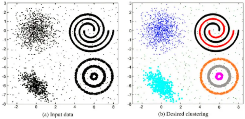
The objective of data clustering, also know as cluster analysis, is to discover the natural groupings of a set of data points, patterns or objects, in-cluding determining of the number of groups and assigning certain individuals into respective groups. An example [9] of clustering is shown in Figure 2.1.

Figure 2.1: Clusters with Diversity

In Figure 2.1 (a), the input data is unlabeled and all the data points, including the scattered dots, circles and swirls, pertain to one large group. After a certain algorithm has been implemented, seven clusters are generated and distinguished by colors in Figure 2.1 (b) with dissimilarities in shape, size and density.

(14)

2.1 Unsupervised Learning

Clustering is a typical unsupervised learning technique. To establish a context, supervised learning will be firstly explained.

Supervised learning is a data mining task of inferring a function from labeled training data. Suppose we observe a response variable Y and m dif-ferent predictor variablesx1, x2, ..., xm, and if there is a potential relationship

between the response Y and the predictors X = (x1, x2, ..., xm), such relation

could be presented in the following general form:

E(Y) =F(X)

In the function above, E(Y) is the expected value of the response Y, F indi-cates the potential but unknown relation.

Under many situations, predictors are readily available, but Y often is hard to get. ThenY could be predicted by:

ˆ

Y = ˆF(X)

where ˆY is the prediction of the response variable, and ˆF is the estimate of the relation between the response and the predictors.

In supervised learning, the goal [10] is to fit a model that relates the response variable to the predictor variables, aiming at accurately predicting the response for future observations (prediction) or better understanding the relationship between the response and the predictors (inference).

(15)

In contrast, unsupervised learning describes a more challenging situa-tion in which for each observasitua-tioni = 1, ..., n, we have a set of measurements

xi but no associated response y. It is unable to fit a predictive model

(re-gression, decision tree, support vector machine, k-nearest neighbor, etc), since observations are unlabeled, and there is no response variable to predict. Such situation is referred to as unsupervised, as a response variable is lacking to supervise the learning.

After classifying learning problems as supervised and unsupervised, semi-supervised learning was proposed, in which a small portion of the train-ing data is labeled, and the unlabeled data, instead of betrain-ing dropped, are also used during the learning process.

2.1.1 Definition of a Cluster

Everitt [11] has studied the cluster and given a specific definition of a cluster by evaluating the circular nature of most proposed definitions. A cluster is a continuous region of variable space containing a relatively high density of data points separated from other high density regions by areas containing a relatively low density of data points.

In clustering problems, things to be clustered are usually called objects or observations, also known as patterns, cases or entities. The aspects of these objects for evaluating their similarities or dissimilarities are often and variously called variables, attributes, features, or characters.

(16)

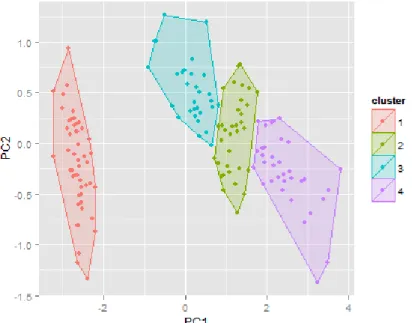
flower dataset, a classical dataset from R. A. Fisher. The iris consists of 150 observations with 4 numerical attributes sepal length, sepal width, pedal length and pedal width, and 1 categorical attribute, species, with 3 categories setosa, versicolor and virginica. In Figure 2.2, after neglecting the categorical attribute, all the data points are grouped into four distinct clusters based on two principal components of numerical characters in the original dataset.

Figure 2.2: Clusters for iris Dataset

There are several characteristics of clusters which could be quantified when observations are plotted as points in a p-dimensional variable space:

(1) Density – the within-cluster points are highly concentrated

(2) Variance – the dispersion from the cluster centroid is small for the points in the cluster

(17)

(3) Dimension – the size or radius of the cluster is small (4) Shape – clusters are typically ellipsoidal

(5) Separation – clusters rarely overlap or they are disconnected. Most of the clustering algorithms are set up based on these characteristics. 2.1.2 General Steps for Cluster Analysis

• Feature Selection: select observations to be clustered and define at-tributes used for clustering such observations

• Proximity Measure: compute similarities or dissimilarities among obser-vations

• Clustering Criterion: express via a cost function or certain rule and choose proper clustering algorithm

• Cluster Generation: create clusters of similar objects

• Cluster Validation: validate the resulting clusters and interpret the result

2.2 Similarities and Dissimilarities

In a data matrix, observations could be thought of as the rows, with attributes as the columns. If the number of observations and attributes are n

and p, respectively, the size of the data matrix would be n×p.

Then the proximity matrix between pairs of observations could be com-puted in terms of the data matrix, it could be either similarity matrix or

(18)

dis-similarity matrix, and typically, correlation is used for computing dis-similarity, while distance is used to measure dissimilarity.

2.2.1 Correlation Coefficients

For the similarity matrix resulting from the data matrixn×p, the entry in row i and column j of the similarity matrix shows how similar (dissimilar) object i and object j are. In this way, the similarity matrix must be n×n.

If correlation is used, the resulting similarity matrix is very different from the ordinary correlation matrix for the same n×p data matrix. In this case, the ordinary correlation matrix would be of size p×p. The entry in row

i and columnj of the ordinary correlation matrix shows how similar variable

i and variable j are in the data matrix. On the other hand, the entry in row

i and column j of a similarity matrix shows how similar observation i and observation j are. That is to say, ann×n similarity matrix shows how similar the rows in the n×p data matrix are, whereas the ordinaryp×p correlation matrix shows how similar the columns in the n×p data matrix are.

So if one observation Xi = {xi1, ...xip} containing p values and

an-other observation Xj = {xj₁, ...x_{j p}} containing p values, and ∀ i, j =

1, ..., n, i6=j, then the sample correlation coefficient for the similarity matrix would be: r=rXiXj = Pp k=1(xik−xi)(xj k−xj) pPp k=1(xik−xi)2 pPp k=1(xj k −xj)2

(19)

Correlation measures are rarely used in practice for computing similar-ities.

2.2.2 Distance Measurements

Most algorithms [12] presume a matrix of dissimilarities with non-negative entries and zero diagonal elements: dii = 0, i = 1,2, ..., n. If the

original data were collected as similarities, a suitable monotone-decreasing function can be used to convert them to dissimilarities. Also, most algorithms assume symmetric dissimilarity matrices, so if the original matrix D is not symmetric, it could turn to be symmetric by replacing it with (D+DT₎_/_2.

Subjectively constructed dissimilarities are seldom distances in the strict sense, since the triangle inequalityd_ii0 ≤d_ik+d

ki0, for allk ∈ {1, ..., n}does not hold.

Thus, some algorithms that assume distances cannot be used with such data. Generally, for ∀i, j, k ∈ 1,2, ..., n, and i 6= j 6= k, the dissimilarity metric such that:

d(i, j)≥0

d(i, i) = 0

d(i, j) =d(j, i)

d(i, j)≤d(i, k) +d(k, j)

And common distance measures for dissimilarities between observations are: (1) Euclidean Distance = pPp_k₌₁(xik−x_{j k})2

(2) Manhattan Distance = Pp

(20)

(3) Mahalanobis Distance = (Xi−Xj) 0

S−1_(X

i−Xj)

where xik is the value of observation i on variable k, x_{j k} is the value of

ob-servation j on variable k, (Xi −Xj) 0

is the 1 ×p row vector of differences between rowiand rowj of the data matrix, andS−1 _{is the inverse of the}_p_×_p

covariance matrix of the attributes of data. And it is standard to standardize variables prior to calculating distance measures used as dissimilarities.

(21)

Chapter 3 Clustering Algorithms

3.1 Connectivity-based Model

Connectivity based clustering, also known as hierarchical clustering, is based on the basic idea of general clustering thoughts that objects are more similar to nearby objects than to objects farther away.

Hierarchical clustering methods require the user to specify a measure of dissimilarity (mostly are the three distance measures introduced in 2.2.2) between disconnected groups of observations. As the name suggests, they produce hierarchical representations, called adendrogram, in which the groups at each level of the hierarchy are generated by merging two lower-level groups. In this way, at the lowest level in this hierarchy, each group contains one single observation; and at the highest level, there is only one group which contains all the data information.

3.1.1 Hierarchical Agglomerative Clustering

There are two basic paradigms for hierarchical clustering: agglomera-tive and divisive. The former paradigm will give a bottom-up dendrogram, while the latter one is expected to show a top-down dendrogram. Four major

(22)

methods are used to compute the similarity of clusters where each of them may contain multiple instances:

• Single Link: Nearest neighbor, clustering two most similar members.

• Complete Link: Farthest neighbor, clustering two least similar members.

• Average Link: Average neighbor, clustering members in average similar-ity.

• Ward’s Method: Minimum variance criterion, clustering objects by min-imizing the total within-cluster variance.

The basic procedures for all of the three methods are similar:

Step 1 Start with clustersC1, C2, ..., Cn, each contains a single observation.

Step 2 Find the proper pair of distinct clusters, sayCi and Cj , mergeCi

and Cj , and decrease the number of clusters by 1.

Step 3 When # cluster equals to 1, stop the process; else, return to Step 2. 3.1.2 Clustering Analysis on Romano-British Pottery

This section clarifies how hierarchical agglomerative clustering works by using the data of Romano-British Pottery [13].

The data shown in Table 3.1 conveys numeric information for the chem-ical composition of Romano-British pottery with 45 specimens, determined by atomic absorption spectrophotometry [14] with the values for nine oxides [15].

(23)

In addition to the chemical composition of the pots, the kiln site at which the pottery was found is categorized into 5 places, with label 1 through 5. Based on such group of data, people would like to know whether, in terms of these chemical compositions, the pots can be divided into distinct clusters, and how these groups are related to the kiln site.

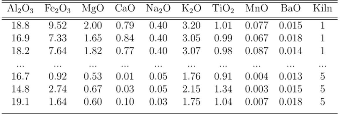
Table 3.1: Romano-British Pottery Data

Al2O3 Fe2O3 MgO CaO Na2O K2O TiO2 MnO BaO Kiln

18.8 9.52 2.00 0.79 0.40 3.20 1.01 0.077 0.015 1 16.9 7.33 1.65 0.84 0.40 3.05 0.99 0.067 0.018 1 18.2 7.64 1.82 0.77 0.40 3.07 0.98 0.087 0.014 1 ... ... ... ... ... ... ... ... ... ... 16.7 0.92 0.53 0.01 0.05 1.76 0.91 0.004 0.013 5 14.8 2.74 0.67 0.03 0.05 2.15 1.34 0.003 0.015 5 19.1 1.64 0.60 0.10 0.03 1.75 1.04 0.007 0.018 5

Among the 45 observations of pottery data, first 21 observations belong to kiln site 1, next 12 observations belong to kiln site 2, next 2 observations kiln site 3, next 5 observations kiln site 4, and the last 5 observations belong to kiln site 5.

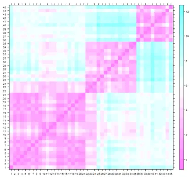
For hierarchical clustering analysis, first, an intuitive impression of the potential clusters of all the 45 specimens of chemical composition of pottery is necessary. In Figure 3.1, the image of dissimilarity matrix of the pottery data using Euclidean distance is given. Each cell of the dissimilarity matrix in the plot has a color-based value from 0 through 12 with color from pink across turquoise, which means the closer to pink the color is, the closer to zero Euclidean distance the cell will be, indicating such group of cells more probably

(24)

belong to the same cluster. Specifically, Figure 3.1 leads to a direct impression that at least 3 clusters exist with much smaller within-cluster distances than those can be seen in other cells.

Figure 3.1: Image of Euclidean Distance based Dissimilarity Matrix on Pottery Data

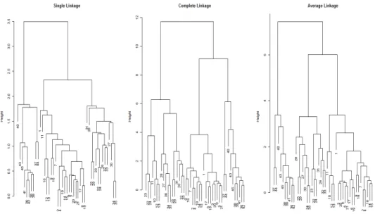
Then, hierarchical agglomerative algorithms is implemented using the first three methods in computing similarities, with dendrograms to visualize the results of hierarchical clustering. This could be realized by the R function hclust, a function specialized in hierarchical cluster analysis. As is shown in Figure 3.2, each dendrogram of single link, complete link and average link, has 3 clusters.

(25)

needs to look for natural groupings defined by long stems. If we cut at height = 2.0 for single link, height = 7.0 for complete link and height = 4.0 for average link, we get exactly 3 clusters in each of the three dendrograms. If Manhattan distance or Mahalanobis distance is used as measurement of dissimilarity, then the dendrograms would be a little bit different.

Figure 3.2: Dendrogram of Hierarchical Clustering using Euclidean Distance In such case, the problem of whether the pots can be divided into distinct clusters has been solved, then the problem of how these clustering relate to kiln sites could also be solved. The relationships between the clusters and the kiln sites could be seen in Table 3.2. Choose the average link as an example, all the 21 pots from Kiln Site 1 belong to Cluster 1; all the 12 pots from Kiln Site 2 and all the 2 pots from Kiln Site 3 are found in Cluster 2; all the pots from Kiln Site 4 and 5 are found in Cluster 3.

(26)

Table 3.2: Relations between Clusters and Kiln Sites for Average Link # Cluster Kiln 1 Kiln 2 Kiln 3 Kiln 4 Kiln 5

1 21 0 0 0 0

2 0 12 2 0 0

3 0 0 0 5 5

3.2 Centroid-based Model

In centroid-based clustering, clusters are represented by a central vec-tor, usually called acentroid, which may not necessarily be an existing member of the current data set. When the number of clustersk is fixed,K-means clus-tering tries to solve such an optimization problem: find the optimalk centroids of potential clusters and assign all the objects to proper centroids in creating clusters, such that the total sum of squared distances between each object and its centroid within a cluster are minimized.

3.2.1 K-means Clustering

Typically, the procedure forK-means clustering would be: Step 1 Randomly pick data points as initial representatives. Step 2 Assign each data point to its closest representative. Step 3 Recompute ”means” for each potential cluster.

In Figure 3.3, an intuitive impression for the procedure ofK-means clustering is shown from left to right. And such procedure is constrained to minimize the total sum of squared distances between data points and the centroid within each cluster, the objective function is given below:

(27)

J = argmin {µ1,...,µk} k X c=1 X i=1,xi∈χc kxi−µck2

where µ1, ..., µk arek centroids, which are the means within each cluster, xi ∈

χc indicates theith data point in thecth cluster, c= 1, ..., k.

Figure 3.3: The WayK-means Clustering Works 3.2.2 K-means Experimental Study on Pottery Data

This section clarifies how K-means clustering works using the same pottery data used in Section 3.1.2. The pottery data is grouped into 1 through 10 clusters, respectively, the values of ”total within-cluster sum of squared distance” for 1 cluster through 10 clusters are listed in Table 3.3.

Table 3.3: Total Within-cluster Sum of Squared Distance

# C 1 2 3 4 5 6 7 8 9 10

SSD 753.7 402.8 145.1 116.8 94.5 74.1 57.6 55.0 55.6 34.1 It can be found in Table 3.3 that the total within-cluster SSD decreases when the data is grouped into 1 cluster through 8 clusters, with the value

(28)

decreases from 753.7 to 55.0. Then the value for such measurement increases a little to 55.6 when there are 9 clusters and drops to 34.1 when there are 10 clusters.

Figure 3.4: Relations between SSD and Number of Clusters

Values in Table 3.3 could be reflected in Figure 3.4, and there is a decreasing trend between number of clusters and the total within-cluster SSD. By means of the ”Elbow” method for determining the number of clusters, the optimal number of clusters using K-means clustering would be three, which matches the number when we use hierarchical agglomerative clustering method based on the same dataset. And when 3 clusters are generated, the explained variance of the clusters (between-cluster SSD) is 80.8 % of the total variance, which is good enough.

(29)

The cluster means in terms of each chemical composition could be found in Table 3.4.

Table 3.4: Cluster Means for Each Cluster

# C Al2O3 Fe2O3 MgO CaO Na2O K2O TiO2 MnO BaO

1 12.44 6.21 4.78 0.21 0.23 4.19 0.68 0.12 0.02 2 17.75 1.61 0.64 0.04 0.05 2.02 1.02 0.03 0.02 3 16.92 7.43 1.84 0.94 0.35 3.10 0.94 0.07 0.02

Meanwhile, a table is available to show the relations between clusters and kiln sites in Table 3.5. All the 12 pots from Kiln Site 2 and all the 2 pots from Kiln Site 3 are found in Cluster 1, all the pots from Kiln Site 4 and 5 are found in Cluster 2, and all the 21 pots from Kiln Site 1 belong to Cluster 3.

Table 3.5: Relations between Clusters and Kiln Sites using K-means # Cluster Kiln 1 Kiln 2 Kiln 3 Kiln 4 Kiln 5

1 0 12 2 0 0

2 0 0 0 5 5

3 21 0 0 0 0

In such case, it is clear that relations between clusters and kiln sites resulted fromK-means clustering in Table 3.5 and those resulted from average link of hierarchical clustering in Table 3.2 are the same, despite the difference in the notation of cluster numbers.

3.2.3 Extensions of K-means

Based on the basic algorithms ofK-means clustering, many extensions have been shown in public. Some of these extensions involves with merging,

(30)

splitting clusters and minimizing the cluster size. Two famous derivation of

K-means in pattern recognition are the ISODATA method by Ball and Hall [16] and the FORGY method by E.W. Forgy [17].

Besides, there’s one significant fact in K-means is that, each data ele-ment is finally assigned to one distinct cluster, clustering in such way is also calledhard clustering. One important extension ofK-means clustering is called Fuzzy c-means, proposed by J.C. Dunn [18] and improved by J.C. Bezdek [19], indicating that each data point can belong (with different amounts of mem-bership level) to multiple cluster. Fuzzy clustering technique is also referred to as soft clustering, compared to hard clustering.

3.3 Model-based Clustering

Model-based clustering, also known as distribution-based clustering, is a general clustering technique based on distribution models. This clustering method defines clusters as observations belonging most likely to the same dis-tribution, and it is similar to the way that some sample data set are generated by Gibbs sampling or MetropolisHastings in Bayesian statistics, by sampling observations from a distribution.

Actually, distribution-based clustering often suffers from a common problem which is overfitting, if there are no constraints set up for the model complexity. In such case, a model with higher complexity for the clustering job would better explain the data, which, at the mean time, add up to the inherent difficulty of choosing the appropriate complexity of the model.

(31)

One effective and commonly used method to solve the problem above is known as Gaussian mixture models, which is often fitted by expectation-maximization algorithm. Specifically, the data set or objects are usually mod-eled with a finite (to avoid overfitting) number of normal distributions, such normal distributions are randomly initialized, and then the initial parameters of such distributions are iterated with multiple runs to reach optimum in order to better fit the data set or objects.

3.3.1 Gaussian Finite Mixture Models

Gaussian finite mixture model is a linear combination of finite number of Gaussian distributions. Several necessary terms related to such model are clarified step by step.

• Gaussian Distribution

Let X be a normally distributed random variable with mean µ and standard deviation σ, for ∀xi ∈ X, i = 1,2, ...., n, the probability function of X would

be: f(xi) =N(xi|µ, σ2) = 1 σ√2πexp{− 1 2( xi−µ σ ) 2_} • Likelihood Function

Then the likelihood function L(µ, σ|xi) of µ and σ for the given x1, x2, ..., xn

would be: L(µ, σ|xi) = n Y i=1 N(xi|µ, σ2)

(32)

• Multivariate Gaussian and Log-likelihood

Let x = {X1, X2, ..., Xn} be a n-dimensional random vector, if every linear

combination of itsn components has a univariate normal distribution, thenX is said to be n-variate normally distributed, with the multivariate Gaussian distribution: x∼Nn(µ,Σ) = _p 1 (2π)n_|_Σ_|exp{− 1 2(x−µ) T_Σ−1_(x₋_µ₎_}

where µ is the n-dimension mean vector with µ = [E[X1],E[X2], ...,E[Xn]],

and Σ is then×n covariance matrix with Σ = [Cov[Xi, Xj]], i= 1,2, ..., n;j =

1,2, ..., n.

Then the log-likelihood function would be:

l(µ,Σ|Xi) = ln n Y i=1 N(Xi|µ,Σ) =−n 2ln|Σ| − 1 2 n X i=1 (Xi−µ)TΣ−1(Xi−µ) + constant (3.1)

Thus, the Maximum Likelihood Estimator ofµand Σ would easily be found: ˆ µ= 1 n n X i=1 Xi ˆ Σ = 1 n n X i=1 (Xi−µ)(Xi−µ)T

(33)

Gaussian finite mixture models is a weighted sum of finite number of Gaussian probability density functions. Suppose we have K multivariate Gaussian distributed random vectorsx1,x2, ...,xK,µkand Σkare each vector’s

mean vector and covariance matrix, then the probability density function for the Gaussian finite mixture model would be:

p(x) =

K

X

k=1

πkN(x|µk,Σk)

whereπk is the weight with

PK

k=1πk = 1, 0≤ πk ≤1, and πk, µk and Σk are

parameters to be estimated. N(x|µk,Σk) is called the kth component model,

each component is a multidimensional Gaussian with its own mean µk and

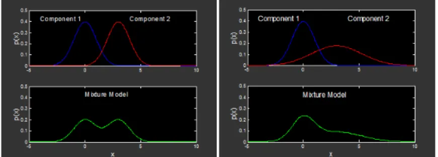
covariance matrix Σk. Figure 3.5 [20] is howp(x) would be like and changing

associated with the change of its parameters.

Figure 3.5: Gaussian Mixture Model with Two Gaussian Distributions Clustering technique based on Gaussian Finite Mixture Models is used to cluster data points generated from each component model. The following two steps are to generate sample data points from each component model, and assign a latent variable to each of the data point.

(34)

Step 1 To generate data points

Firstly, randomly pick one of the components with probability πk, then draw

a sample data points xi, i= 1,2, ..., n from that component distribution

Step 2 Assign a latent variable to each data point

After each data point is generated from one of the K components, a latent variable zi = (zi1, zi2, ..., ziK) is associated with each xi, where PK_k₌₁ and

p(ziK = 1) =πk

Since the probability density function of Gaussian finite mixture model is already given, then the log-likelihood function for the generated data points from the Gaussian mixture is not hard to find:

l(π, µ,Σ|x) = lnL(π, µ,Σ|x) = ln n Y i=1 K X k=1 πkN(xi|µk,Σk) = n X i=1 ln{ K X k=1 πkN(xi|µk,Σk)} (3.2)

Right now, values of the latent variables, which are associated with data points xi, are not known, then the maximization of the incomplete log

likeli-hood is needed, and Expectation-Maximization (EM) algorithm can be used to estimate the mixture parameters πk, µk and Σk by iteratively maximizing

(35)

3.3.2 Expectiation-Maximizations Clustering

The ExpectationMaximization (EM) algorithm is an iterative method for finding estimates of parameters by maximizing the log-likelihood in statis-tical models, which depend on unobserved latent variables. The EM iteration alternates between performing an expectation step (E-step) and a maximiza-tion step (M-step), where the E-step creates a funcmaximiza-tion for the expectamaximiza-tion of the log-likelihood which is evaluated by the current estimate for the pa-rameters, and the M-step computes estimate of parameters by maximizing the expected log-likelihood resulted from the E-step. The parameter-estimates obtained from the M-step are then used to determine the distribution of the latent variables in the next E- step.

For the Gaussian Finite Mixture Model given in Section 3.3.1, the spe-cific expectation and maximization steps are as follows.

• E-step: evaluate ”responsibilities” of each cluster of data points with the current parameters

For the given initial parameters, it is doable to compute the expected values of the latent variables using Bayes Theorem, such values are also known as responsibilities of the data points.

(36)

where responsibilitiesτik ∈[0,1] and PK_k₌₁τik = 1 for all i.

• M-step: re-estimate parameters using the existing ”responsibilities”

Use the responsibilities to maximize the expected complete log-likelihood to give parameter updates.

Combine Equation 3.2 and Equation 3.3, then the maximum likelihood estimator with responsibilities for the parameters could be found:

∂l(π, µ,Σ|x) ∂µk = n X i=1 πkN(xi|µk,Σk) PK k=1πkN(xi|µk,Σk) Σ−_k1(xk−µk) = 0 = n X i=1 τikΣ−_k1(xi−µk) = 0 (3.4) µk = Pn i=1τikxi Pn i=1τik

Similarly, optimizations ofπk and Σk are as follows:

πk =

Pn

i=1τik

(37)

Σk =

Pn

i=1τik(xi−µk)(xi−µk)T

Pn

i=1τik

After the estimates for the parameters are obtained, iterate E-step and M-step until the log-likelihood of data does not increase any more-reach max-imum of log-likelihood, in such case, parameters are iteratively optimized to fit the data set.

In order to obtain a hard clustering, objects or data points are often then assigned to the Gaussian distribution they most likely belong to, for soft clustering, this is not necessary.

Model-based clustering produces complex models for clusters that can capture correlation and dependence between attributes. However, there’s one obvious limitation for users: for many real data sets, there may be no well-defined distribution model, that is to say, for example, Gaussian distributed is a strong assumption on the data.

3.3.3 Experimental Analysis on iris Dataset

As is used in Section 2.1.1 as an example of clusters, the iris dataset here is another good example to show how model-based clustering works, espe-cially the Gaussian finite mixture model fitted by Expectation-Maximization clustering algorithm.

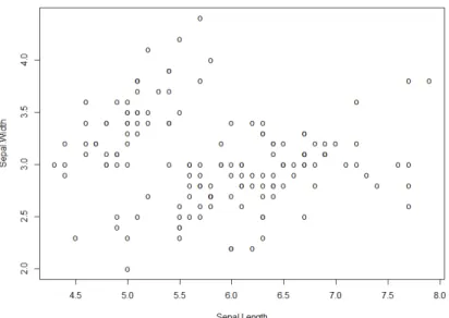
In this section, only the first two columns Sepal.Length and Sepal.Width fromirisare used, since the data with two dimensions makes the analysis more friendly to visualize. The bivariate iris dataset is shown in Figure 3.6.

(38)

Figure 3.6: The Bivariate iris Dataset

(39)

And from the density estimate for the data in Figure 3.7, a relatively obvious mixture model with 2 Gaussian distributions can be seen, thus, the clustering technique Gaussian Finite Mixture Model fitted by EM algorithm is suitable to be operated on the data.

The R package mclust [21] is used, which is specialized in normal mixture modeling for model-based clustering, classification, and density esti-mation. The functionMclustperforms clustering analysis based on Gaussian finite mixture model fitted by EM clustering, and a brief result in shown in Table 3.6, the corresponding plots are shown in Figure 3.8

Table 3.6: Brief Results of EM Clustering

Log-likelihood Observations DF BIC Clustering Table -225.9263 150 10 -501.9589 #1: 49, #2: 101 In this case, the best model according toBICis an variable-covariance model with 2 clusters, the maximum loglikelihood is 225.9263, optimal BIC -501.9589, and 49 observations belong to Cluster 1 and 101 observations belong to Cluster 2.

Additionally, parameters π, µ,Σ in the Gaussian finite mixture model could be found by EM iterations which are shown in Table 3.7 and Table 3.8

Table 3.7: Parameter Estimates of Mixing Probabilities and Means Cluster # Mixing Probability π Means µ

1 0.3223103 S.L: 5.016245; S.W: 3.454680 2 0.6776897 S.L: 6.236698; S.W: 2.868354

(40)

Table 3.8: Parameter Estimates of Covariances Cluster # 1 Σ Sepal.Length Sepal.Width

Sepal.Length 0.12129045 0.09030555 Sepal.Width 0.09030555 0.11938505 Cluster # 2 Σ Sepal.Length Sepal.Width

Sepal.Length 0.4643624 0.1251138 Sepal.Width 0.1251138 0.1117615

In the mean time, the formation of the two clusters could be found using function classification in mclust package: observation 1 through 41 and observation 43 though 50 are grouped in Cluster 1, and rest of the total 150 observations belong to Cluster 2.

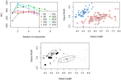
Figure 3.8: Plots Associated with the Function Mclust foriris dataset Figure 3.8 shows three plots resulted from theMclust function in the mclust package.

(41)

Upper left: Change of BIC from for the 10 available model parameterizations as the increase of the number of clusters up to 9. Different symbols and line types indicate different model parameterizations. Thebest model is thought of as the one with the highest BIC among the fitted models. Combined with Table 3.6, it is known that the optimal BIC -501.9589 is reached at the best number of clusters 2, by the VEV model, which specifically is a Ellipsoidal Gaussian mixture model with variable volume, equal shape and variable orientation. Upper right: The specific clustering of iris data, with different symbols indicating diverse clusters corresponding to the best model as determined by function Mclust. The mean values for each cluster are marked and ellipses with axes are drawn corresponding to their covariances. In such case, there are two clusters, each with a different covariance.

Lower center: A projection of the iris data showing the uncertainty for the clustering. Larger and dark symbols indicate more uncertain observations. As is shown in the this plot, uncertain observations occur with higher frequencies at the boundaries between two clusters.

(42)

Chapter 4 Cluster Validation

4.1 Determination of Number of Clusters

Determining the number of clusters for a dataset, as illustrated in Chap-ter 2, is one of the two major concerns in clusChap-tering analysis, and also a frequent problem in data clustering. The quantity is often labeledk as in the K-means algorithm.

The appropriate choice of kis often fuzzy, with interpretations depend-ing on the shape and scale of the data points’ distribution and the desired clus-tering resolution of the user, which sometimes could be subjective. Actually, increasing k without penalty will always reduce the amount of within-cluster sum of squared distance in the resulting clustering, and in the mean time, in-crease the amount of between-cluster sum of squared distance, improving the percentage of explained variance for the clustering.

Under the extreme clustering situation of zero within-cluster sum of squared distance, each data point is thought of as its own cluster, thenkequals the size of the data. In such case, the highest proportion of explained variance has been reached, however, leading the clustering to be meaningless, since without clustering, each original data point is its own ”cluster”. Therefore,

(43)

the optimal choice ofk will strike a trade-off balance between a high volume of explained variance of clusters and a relatively small number of clusters. There are several categories of methods for making this decision.

4.1.1 Invalidity of Statistical Significance Testing

Firstly, one method which is commonly used but theoretically invalid for determining the number of clusters should be explained, the method is statistical significance testing, like F test based on ANOVA. Unlike many other statistical procedures, most clustering algorithms are used when there are no prior hypotheses, and cluster analysis isstructure-imposing, sometimes it will find clusters even if none exist. Consequently, F tests are almost always misleadingly significant.

4.1.2 The Elbow Method

The elbow method looks at the proportion of variance explained as a function of the number of clusters k. An ideal value of k such that adding another cluster doesn’t give much better goodness of fit of the data. In partic-ular, if the percentage of variance explained by the clusters is drawn against the number of clusters, the first added cluster will provide much explained information (explained variance), but at some point the marginal gain will inevitably drop, giving an angle in the plot. The number of clusters is chosen right at this point, which is the ”elbow criterion”. This ”elbow” cannot always be unambiguously identified [22].

(44)

Percentage of the explained variance is the ratio of the between-cluster variance to the total variance. A slight variation of this method plots the curvature of the within-cluster variance [23], and Figure 3.4 in Section 3.2.2 is an example of such variation of the regular elbow method. The example of the regular elbow method for determining the number of clusters, compared to Figure 3.4, could be seen in Figure 4.1, which is based on the same dataset of Romano-British Pottery [24].

Figure 4.1: Explained Variance by Clustering against Number of Clusters The explained variance of clustering, which is calculated as the between-cluster sum of squared distance divided by the total sum of squared distance, reaches the ”elbow” when the number of clusters is three, which is the same result obtained in Figure 3.4.

(45)

At this time, 80.8 % of the total variance is explained, which is good enough and can be found in Table 4.1. When the number of clusters increases from 3 to 4, it does not add much (only 3.7%) increase in the percentage of explained variance. Thus, 3 clusters would be an ideal solution for clustering the pottery data usingK-means algorithm.

Table 4.1: Percentage of Explained Variance against Number of Clusters

# C 1 2 3 4 5 6 7 8 9 10

% ≈0 46.6 80.8 84.5 87.5 90.2 92.4 92.7 92.6 95.5

4.1.3 Information Criterion Approach

Another set of methods for number of clusters determination are the in-formation criteria, such as the Akaike inin-formation criterion (AIC) or Bayesian information criterion (BIC), which are often used as means for model selec-tion in statistical modeling or predictive modeling if it is possible to construct the likelihood function for the clustering model. For example: The K-means model to some extent is a Gaussian mixture model, and the likelihood for the Gaussian mixture model is not hard to find and then also the information criterion values [25].

4.1.4 Three Top Performing Heuristic Methods

Milligan and Cooper [26] [27] developed three heuristic methods in their studies to determine the number of clusters, which are cubic clustering criterion (CCC), pseudo-F statistic and pseudo-T2 _{statistic. All the three criterion or}

(46)

statistic have been implemented into the statistical software SAS, and could been obtained by SAS commandPROC CLUSTER.

• Cubic Clustering Criterion (CCC): the local peaks in CCC when plotted against the number of clusters provide a list of candidates for k.

• Pseudo-F Statistic: measures the separation among all clusters, and the local peaks in pseudo-F statistic when plotted against the number of clusters would would provide a list of candidates for k.

• Pseudo-T2 Statistic: measures the separation between the two clusters most recently joined, when the pseudo-T2 is plotted against the number of clusters, the number to be one more than the peaks (or end of a run of large values) of pseudo-T2 _{would provide a list of candidates for}_k_.

Since in each of the above method, the number of local peaks may be more than one, then the three heuristic methods only provide a list of candidates for the number of clusters. In order to determine the optimal choice of k, the underlying theory of the subject being studied should be paid attention to, and other approaches for determining the k need to be used associated with the heuristic methods.

4.2 Cluster Validation

When clustering procedures are completed and the clustering results are obtained with a confirmed number of clusters and an assignment of data

(47)

points into each cluster, the next and also the final step is to evaluate the goodness of the resulting clusters, which is also known as cluster validation, and cluster validation usually is associated with the process of determining the number of clusters.

As for the motivation of cluster validation, it involves several concerns: to avoid finding clusters in noise, to compare different clusters, or to compare the effectiveness of different clustering algorithms on a specific dataset. One potentially useful validation technique isCross-validation.

For cross-validation, firstly, randomly split the observations, and then choose one clustering technique to perform cluster analysis on each set of ob-servations. If similar clusters develop, then such clustering result is potentially good to accept. However, if different clusters appear, then the clustering result is not generalizable. A variation on this method is to perform cluster analysis (specifically, using K-means algorithm) on the first set of observations, then use its cluster centroids as seeds to cluster the second set. This forces the same number of clusters in the cross-validation. If the cluster centroids from the first set reproduce similar assignments of data points and the clusters in the second set of observations, which have small within-cluster errors and big between-cluster errors, then this would be a good clustering.

Halkidi, et al [28] introduced the fundamental concepts of cluster va-lidity, such ascompactness and separation, and gave a systematic analysis of how cluster validity indices are used in cluster validation, including external criteria, internal criteria and relative criteria.

(48)

Brook, et al [29] developed an R packageclValidwhich contains specific functions for validating the clustering results. There are three main types of cluster validation measures available which are ”internal”, ”stability”, and ”biological”, and such package can evaluate the cluster analysis resulted from up to 9 clustering algorithms, including hierarchical,K-means, self-organizing maps (SOM), model-based clustering, etc.

(49)

(50)

Appendix A

R Code for Figure 2.2 & Clustering Analysis

on Romano-British Pottery

## F i g u r e 2 . 2 C l u s t e r s f o r i r i s D a t a s e t on Page 6 l i b r a r y ( d e v t o o l s ) i n s t a l l g i t h u b ( ’ s i n h r k s / g g f o r t i f y ’ ) l i b r a r y ( g g p l o t 2 ) l i b r a r y ( g g f o r t i f y ) l i b r a r y ( c l u s t e r ) s e t . s e e d ( 1 ) a u t o p l o t ( f a n n y ( i r i s [−5 ] , 4 ) , frame = TRUE) ## C l u s t e r i n g A n a l y s i s on Romano−B r i t i s h P o t t e r y ## on Page 14−16 l i b r a r y (HSAUR) k i l n <− r e p ( 1 : 5 , c ( 2 1 , 1 2 , 2 , 5 , 5 ) ) k i l n <− a s . d a t a . frame ( k i l n ) p o t t e r y [ , 1 0 ] <− k i l n p o t t e r y d i s t <− d i s t ( p o t t e r y [ , c o l n a m e s ( p o t t e r y ) != ” k i l n ” ] , method = ” e u c l i d e a n ” ) # F i g u r e 3 . 1 : Image o f E u c l i d e a n D i s t a n c e b a s e d # D i s s i m i l a r i t y Matrix on P o t t e r y Data l i b r a r y ( l a t t i c e ) l e v e l p l o t ( a s . m a t r i x ( p o t t e r y d i s t ) , x l a b = ”Number o f Pot ” , y l a b = ”Number o f Pot ” )

p o t t e r y s i n g l e <− h c l u s t ( p o t t e r y d i s t , method = ” s i n g l e ” )

p o t t e r y c o m p l e t e <− h c l u s t ( p o t t e r y d i s t , method = ” c o m p l e t e ” )

(51)

p o t t e r y a v e r a g e <− h c l u s t ( p o t t e r y d i s t , method = ” a v e r a g e ” )

# Table 3 . 2 : R e l a t i o n s between C l u s t e r s and K i l n S i t e s # f o r Average Link c l u s t e r s <− c u t r e e ( p o t t e r y a v e r a g e , h = 4 ) x t a b s ( ˜ c l u s t e r s + k i l n , d a t a = p o t t e r y ) # F i g u r e 3 . 2 : Dendrogram o f H i e r a r c h i c a l C l u s t e r i n g # u s i n g E u c l i d e a n D i s t a n c e par ( mfrow =c ( 1 , 3 ) )

p l o t ( p o t t e r y s i n g l e , main = ” S i n g l e Link ” , sub = ” ” , x l a b = ” ” )

p l o t ( p o t t e r y c o m p l e t e , main = ” Complete Link ” , sub = ” ” , x l a b = ” ” )

p l o t ( p o t t e r y a v e r a g e , main = ” Average Link ” , sub = ” ” , x l a b = ” ” )

(52)

Appendix B

R Code for

K

-means Experimental Study on

Pottery Data

## K−means E x p e r i m e n t a l Study on P o t t e r y Data on ## Page 17−19 l i b r a r y ( g g p l o t 2 ) l i b r a r y (HSAUR) l i b r a r y (HSAUR2) s e t . s e e d ( 1 3 ) r e s . kmeans <− l a p p l y ( 1 : 1 0 , f u n c t i o n ( i ) { kmeans ( p o t t e r y [ , 1 : 9 ] , c e n t e r s = i ) }) #Within SS f o r e a c h c l u s t e r ( 1 c l u s t e r t o 10 c l u s t e r s ) l a p p l y ( r e s . kmeans , f u n c t i o n ( x ) x $ w i t h i n s s )

#Table 3 . 3 : T o t a l Within−c l u s t e r Sum o f Squared D i s t a n c e r e s . w i t h i n . s s <− s a p p l y ( r e s . kmeans , f u n c t i o n ( x )

sum ( x $ w i t h i n s s ) ) r e s . w i t h i n . s s

#F i g u r e 3 . 4 : R e l a t i o n s between SSD and Number o f C l u s t e r s g g p l o t ( d a t a . frame (No . o f C l u s t e r s = 1 : 1 0 ,

SSD = r e s . w i t h i n . s s ) ,

a e s (No . o f C l u s t e r s , SSD ) ) + g e o m p o i n t ( ) + g e o m l i n e ( ) + s c a l e x c o n t i n u o u s ( b r e a k s = 0 : 1 0 ) #Table 3 . 4 : C l u s t e r Means f o r Each C l u s t e r &

(53)

#u s i n g K−means r e s . kmeans [ 3 ] ## Table 4 . 1 : P e r c e n t a g e o f E x p l a i n e d V a r i a n c e a g a i n s t ## Number o f C l u s t e r s on Page 35 r e s . between . s s <− s a p p l y ( r e s . kmeans , f u n c t i o n ( x ) ( x $ b e t w e e n s s ) / ( x $ t o t s s ) ) r e s . between . s s # F i g u r e 4 . 1 : E x p l a i n e d V a r i a n c e by C l u s t e r i n g a g a i n s t # Number o f C l u s t e r s on Page 34 g g p l o t ( d a t a . frame (No . o f C l u s t e r s = 1 : 1 0 , BSS in TOTSS = r e s . between . s s ) , a e s (No . o f C l u s t e r s , BSS in TOTSS ) ) + g e o m p o i n t ( ) + g e o m l i n e ( ) + s c a l e x c o n t i n u o u s ( b r e a k s = 0 : 1 0 )

(54)

Appendix C

R Code for Experimental Analysis on iris

Dataset

## E x p e r i m e n t a l A n a l y s i s on I r i s D a t a s e t on Page 28−30 l i b r a r y ( m c l u s t )

i m c l u s t <− Mclust ( i r i s [ , 1 : 2 ] )

# Table 3 . 6 : B r i e f R e s u l t s o f EM C l u s t e r i n g &

# Table 3 . 7 : Parameter E s t i m a t e s o f Mixing P r o b a b i l i t i e s # and Means

# Table 3 . 8 : Parameter E s t i m a t e s o f C o v a r i a n c e s summ <− summary ( i m c l u s t , p a r a m e t e r s = TRUE) summ i m c l u s t $ B I C i m c l u s t $ c l a s s i f i c a t i o n # F i g u r e 3 . 6 : The B i v a r i a t e i r i s D a t a s e t p l o t ( i r i s $ S e p a l . Length , i r i s $ S e p a l . Width , x l a b = ” S e p a l . Length ” , y l a b = ” S e p a l . Width ” , pch = ” o ” ) # F i g u r e 3 . 7 : D e n s i t y E s t i m a t e f o r B i v a r i a t e i r i s D a t a s e t i r i s D e n s <− d e n s i t y M c l u s t ( i r i s [ , 1 : 2 ] ) p l o t ( i r i s D e n s , t y p e = ” p e r s p ” , c o l = g r e y ( 0 . 8 ) ) # F i g u r e 3 . 8 : P l o t s A s s o c i a t e d w i t h t h e F u n c t i o n Mclust # f o r i r i s D a t a s e t p l o t ( i m c l u s t )

(55)

Bibliography

[1] Wikipedia, “Cluster analysis - wikipedia, the free encyclopedia,” 2015, [Online; accessed 15-February-2015]. [Online]. Available: http://en.wikipedia.org/wiki/Cluster analysis

[2] R. C. Tryon,Cluster analysis: correlation profile and orthometric (factor) analysis for the isolation of unities in mind and personality. Edwards brother, Incorporated, lithoprinters and publishers, 1939.

[3] R. B. Cattell, “The description of personality: basic traits resolved into clusters.” The journal of abnormal and social psychology, vol. 38, no. 4, p. 476, 1943.

[4] R. O. Duda, P. E. Hart, and D. G. Stork, Pattern classification. John Wiley & Sons, 2012.

[5] O. Chapelle, B. Sch¨olkopf, A. Zienet al.,Semi-supervised learning. MIT Press Cambridge, 2006.

[6] T. Lange, M. H. Law, A. K. Jain, and J. M. Buhmann, “Learning with constrained and unlabelled data,” inComputer Vision and Pattern Recog-nition, 2005. CVPR 2005. IEEE Computer Society Conference on, vol. 1. IEEE, 2005, pp. 731–738.

(56)

[7] S. Basu, A. Banerjee, and R. J. Mooney, “Active semi-supervision for pairwise constrained clustering.” inSDM, vol. 4. SIAM, 2004, pp. 333– 344.

[8] M. Bilenko, S. Basu, and R. J. Mooney, “Integrating constraints and met-ric learning in semi-supervised clustering,” inProceedings of the twenty-first international conference on Machine learning. ACM, 2004, p. 11. [9] A. K. Jain, “Data clustering: 50 years beyond k-means,” Pattern

recog-nition letters, vol. 31, no. 8, pp. 651–666, 2010.

[10] J. Gareth, An Introduction to Statistical Learning: with Applications in R. Springer, 2013.

[11] B. S. Everitt, “Unresolved problems in cluster analysis,”Biometrics, pp. 169–181, 1979.

[12] T. Hastie, R. Tibshirani, J. Friedman, T. Hastie, J. Friedman, and R. Tib-shirani,The elements of statistical learning. Springer, 2009, vol. 2, no. 1. [13] T. Hothorn and B. S. Everitt,A handbook of statistical analyses using R.

CRC Press, 2014.

[14] Wikipedia, “Atomic absorption spectroscopy - wikipedia, the free ency-clopedia,” 2015, [Online; accessed 07-March-2015]. [Online]. Available: http://en.wikipedia.org/wiki/Atomic absorption spectroscopy

(57)

[15] A. Tubb, A. Parker, and G. Nickless, “The analysis of romano-british pottery by atomic absorption spectrophotometry,”Archaeometry, vol. 22, no. 2, pp. 153–171, 1980.

[16] G. H. Ball and D. J. Hall, “Isodata, a novel method of data analysis and pattern classification,” DTIC Document, Tech. Rep., 1965.

[17] E. W. Forgy, “Cluster analysis of multivariate data: efficiency versus interpretability of classifications,”Biometrics, vol. 21, pp. 768–769, 1965. [18] J. C. Dunn, “A fuzzy relative of the isodata process and its use in detecting

compact well-separated clusters,” 1973.

[19] J. C. Bezdek,Pattern recognition with fuzzy objective function algorithms. Kluwer Academic Publishers, 1981.

[20] S. Padhraic, “A guided tour of finite mixture models: From pearson to the web.” Presented as the ICML 01 Keynote Talk at Williams College, 2001.

[21] C. Fraley, A. E. Raftery, T. B. Murphy, and L. Scrucca, “mclust version 4 for r: Normal mixture modeling for model-based clustering, classification, and density estimation,” 2012.

[22] D. J. Ketchen and C. L. Shook, “The application of cluster analysis in strategic management research: an analysis and critique,”Strategic man-agement journal, vol. 17, no. 6, pp. 441–458, 1996.

(58)

[23] C. Goutte, P. Toft, E. Rostrup, F. ˚A. Nielsen, and L. K. Hansen, “On clustering fmri time series,”NeuroImage, vol. 9, no. 3, pp. 298–310, 1999. [24] T. Hothorn and B. S. Everitt,A handbook of statistical analyses using R.

CRC Press, 2014.

[25] C. Goutte, L. K. Hansen, M. G. Liptrot, and E. Rostrup, “Feature-space clustering for fmri meta-analysis,” Human brain mapping, vol. 13, no. 3, pp. 165–183, 2001.

[26] G. W. Milligan and M. C. Cooper, “An examination of procedures for determining the number of clusters in a data set,”Psychometrika, vol. 50, no. 2, pp. 159–179, 1985.

[27] M. C. Cooper and G. W. Milligan, The effect of measurement error on determining the number of clusters in cluster analysis. Springer, 1988. [28] M. Halkidi, Y. Batistakis, and M. Vazirgiannis, “On clustering validation

techniques,”Journal of Intelligent Information Systems, vol. 17, no. 2-3, pp. 107–145, 2001.

[29] G. Brock, V. Pihur, S. Datta, and S. Datta, “clvalid, an r package for cluster validation,” Journal of Statistical Software (Brock et al., March 2008), 2011.

(59)

Vita

Lihao Zhang was born in Liaocheng, China in 1990. He received the Bachelor of Science degree in Mathematics and Applied Mathematics from Shandong University, China in 2013. He was accepted to the Master’s program in Statistics in The University of Texas at Austin in 2013, and then he started his graduate studies.

Permanent address: [email protected]

This report was typeset with LA_TEX† _{by the author.}

†_LA_{TEX is a document preparation system developed by Leslie Lamport as a special} version of Donald Knuth’s TEX Program.