Kent Academic Repository
Full text document (pdf)
Copyright & reuse
Content in the Kent Academic Repository is made available for research purposes. Unless otherwise stated all
content is protected by copyright and in the absence of an open licence (eg Creative Commons), permissions
for further reuse of content should be sought from the publisher, author or other copyright holder.
Versions of research
The version in the Kent Academic Repository may differ from the final published version.
Users are advised to check
http://kar.kent.ac.uk
for the status of the paper.
Users should always cite the
published version of record.
Enquiries
For any further enquiries regarding the licence status of this document, please contact:
[email protected]
If you believe this document infringes copyright then please contact the KAR admin team with the take-down
information provided at
http://kar.kent.ac.uk/contact.html
Citation for published version
Rashid, Tabish and Agrafiotis, Ioannis and Nurse, Jason R. C. (2016) A New Take on Detecting
Insider Threats: Exploring the use of Hidden Markov Models. In: 8th ACM CCS International
Workshop on Managing Insider Security Threats (MIST), October 28, 2016, Vienna, Austria.
DOI
https://doi.org/10.1145/2995959.2995964
Link to record in KAR
http://kar.kent.ac.uk/67482/
Document Version
Author's Accepted Manuscript
A New Take on Detecting Insider Threats:
Exploring the use of Hidden Markov Models
Tabish Rashid
Department of Computer Science, University of Oxford [email protected]Ioannis Agrafiotis
Department of Computer Science, University of Oxford [email protected]Jason R. C. Nurse
Department of Computer Science, University of Oxford [email protected]ABSTRACT
The threat that malicious insiders pose towards organisa-tions is a significant problem. In this paper, we investigate the task of detecting such insiders through a novel method of modelling a user’s normal behaviour in order to detect anomalies in that behaviour which may be indicative of an attack. Specifically, we make use of Hidden Markov Models to learn what constitutes normal behaviour, and then use them to detect significant deviations from that behaviour. Our results show that this approach is indeed successful at detecting insider threats, and in particular is able to accu-rately learn a user’s behaviour. These initial tests improve on existing research and may provide a useful approach in addressing this part of the insider-threat challenge.
Keywords
Insider threat; Anomaly detection system; Machine learning
1.
BACKGROUND AND RELATED WORK
Organisational computer systems are increasingly threat-ened by insiders. The Breach Level Index, which tracks publicly disclosed breaches, shows that almost 40% of data breaches are attributed to malicious insiders or accidental loss due to insiders [6]. It is evident that insider threats now represent a significant portion of the cyber-attacks an organisation faces, even if we do not take into account the unreported incidents. In addition, they are often the most costly type of attack [14] due to the elevated level of trust and access that an insider is afforded.
As insider threats have become more prevalent, there have been numerous advances in both industry and research to-wards attack prevention and detection. At the programme level, the CERT division at CMU maintains a comprehensive research directive on insider threats, and are considered pio-neers in the field [2]. One of the major tools used in explor-ing insider threat by CERT is System Dynamics diagrams, which aid in defining relationships between different precur-sors and factors indicative of an attack. Instead of
sepa-ACM ISBN XXXXXXXXXX.
DOI:http://dx.doi.org/10.1145/2995959.2995964
rately modelling different types of insider attacks as done in the CERT models, a unifying framework to characterise insider attacks has been presented in [11]. The framework is particularly powerful for analysing cases, in order to under-stand behaviours that may lead to an attack, the reasons for an attack, the types of attacks that may be launched, and most importantly, to compare this data across other cases.
The U.S. Department of Homeland Security published a report in 2014: “Combating the Insider Threat”[4]. The report is primarily concerned with the behavioural aspects of the insider threat, and how certain traits can indicate an increased likelihood of a threat. The authors suggest that one of the best prevention measures is educating in-dividuals to report certain behaviours that they observe in their peers. These “Characteristics of Insiders at Risk of Becoming a Threat” are vague (Ethical Flexibility, Introver-sion, etc.) and can often be hard to quantify. In the report they also provide a short list of behavioural indicators which could signal an insider threat, such as “Remotely accesses the network while on vacation, sick or at odd times”, which are easier to observe. Underscoring all of this advice is the concept of a baseline of normal behaviour, which is a prereq-uisite in attempting to observe significant levels of deviation of a certain behaviour.
Machine learning-based approaches have been central to work on insider-threat detection. The actions that an em-ployee takes over a period of time on a system (e.g., logging on/off, file accesses, etc.) can be modelled as a sequence. The sequences that are seen often or on a usual basis, can then be considered as the user’s normal behaviour. Ob-served actions which do not resemble those normal sequences can be regarded as anomalous behaviour, which then may indicate a potential insider threat or at least an event to be investigated. This is the approach proposed by Parveen and Thuraisingham [13]. They extend this line of reasoning, and introduce “concept-drift”, which is the gradual change in a user’s actions over time. They postulate that this more ac-curately detects anomalous behaviour, since a user’s actions often change over time (due to increasing skill or responsi-bility), and these changes would be regarded as anomalous in a model which did not account for the drift. This is a sen-sible assumption to make as it strictly generalises the static behavioural approach, and also introduces the flexibility and adaptability that is expected of machine learning.
In addition to using data collected on a user‘s actions, the literature on characterising the insider threat suggests that behavioural and personality characteristics are equally (if not more) important. Brdiczka et al. [1], combine structural To be published in proceedings of the 8th ACM CCS International Workshop on Managing Insider Security Threats (MIST)
anomaly detection with psychological profiling, in order to reduce the rate of false positives compared to using anomaly detection alone. Under the assumptions that the majority of users in a data set are not malicious insiders, and that their common patterns define normalcy, they propose the use of graph partitioning algorithms in order to discover a user’s regular patterns.
The assumption that the majority of users are not threats is common in the literature, as is taking a user‘s common patterns as normalcy. However, whether it is necessary to adjust the baseline of normalcy over a period of time is of-ten contested in the literature. On the one hand it is argued that a user‘s actions are constantly evolving and that this is not indicative of anomalous behaviour[13, 12], whereas oth-ers [18, 3] proceed without adjusting their baseline and still obtain good results. We are of the opinion that a learning-based approach which modifies the baseline is advantageous, and should be pursued whenever possible.
In this paper we attempt to extend existing work and pro-pose a novel approach to detect insider threats. In particu-lar, we aim to build on the approach to anomaly detection via modelling a user’s normal behaviour as a sequence ([13]) through the use of Hidden Markov Models (HMMs) [15]. HMMs provide algorithms for learning parameters from a set of observed sequences, and also for predicting the prob-ability of observing a given sequence. Previous research has demonstrated how HMMS may be used to design intru-sion detection systems that either detect attacks on system calls into the kernel of an operating system [20] or novel n-grams in computer audit [10] or in more recent research code-reuse attacks executing maliciously intended instruc-tion sequences [22]. Thus, they are an ideal candidate for consideration in our goal of insider-threat detection. We can use them to learn parameters as more sequences are ob-served, and also to classify sequences as anomalous (thus potentially indicative of a concerning insider event) if their probability of observation is significantly low. To the best of our knowledge, we are the first articles to consider the use of this approach to detect insider threats.
The remainder of this article is structured as follows. Sec-tion 2 presents the research context including the motivaSec-tion for using HMMs and the feature set we will consider for our implementation and experimentation. Next, in Section 3 we detail our approach and implementation, and discuss algo-rithms used and how we train our model to detect insider threats. This is then followed by a report on the validation exercises and case study conducted in Section 4. Finally we conclude in Section 5, also presenting limitation of our work and outlining avenues for future research.
2.
RESEARCH CONTEXT
2.1
Overview
As discussed in Section 1, we will approach the problem of insider-threat detection through the modelling of a user’s normal behaviour and then searching for anomalies in that behaviour. A sequence is a natural choice for modelling ac-tions and events through time, and so the difficulty becomes one of finding anomalous sequences in a dataset.
Hidden Markov Models (HMM) have been used exten-sively in areas such as Computational Linguistics and Bioin-formatics due to their temporal pattern recognition capabili-ties. They are well suited to capturing sequential behaviour
and have had many successes in the analysis of biological sequences and recognising patterns in language [15]. HMMs provide algorithms for learning parameters from a set of ob-served sequences, and also for predicting the probability of observing a given sequence. This differs to approaches such as One-class Support Vector Machines (OCSVM), which are a type of SVM in which the algorithm attempts to separate the data points from the origin via a hyperplane of maxi-mum distance from the origin [16].
Let us consider a simple example in order to illustrate the difference in functionality of HMMs over other ML tech-niques such as a One-Class Support Vector Machine (SVM) when sequential patterns in data is of importance. Assume data consisting of 19 sequences which are generated by re-peating{1,0,0,1}between 1 and 4 times, as well as a single sequence which repeats {1,0,2,1} 2 times. We intend for this dataset to represent basic actions carried out over a time period. The fictional user performs normal actions for 16 time steps, then an anomalous action (indicated by the 2) followed by 3 more normal actions. Thus, the anomalous sequence is the 17thsequence in the dataset.
Figure 1: The results of running the HMM and One-Class SVM on our example dataset
In order to make use of a One-Class SVM we must pad our sequences to all be of length 16 (interpreted as 16 dimen-sional vectors by the SVM, which is the maximum length of a sequence in our dataset). We would then train the SVM on the entire dataset as a whole, and ask it to classify in-stances as anomalous (−1) or normal (+1). Conversely, for the HMM we would train it on the first instance, and then feed it the remaining sequences one by one and ask it to pre-dict their log likelihood, and also to learn from them. This therefore represents a somewhat more intelligent approach when sequence in which actions occur are of importance.
Figure 1 shows the results of running both models. It is evident from Figure 1 that the HMM is superior, not only because it clearly identifies the anomalous sequence but also
since it is much better suited to handling temporal infor-mation. The SVM has no concept of a temporal relation between the sequences, nor does it handle variable length sequences well. We have considered only One-Class SVMs as they are representative of fixed-length vector based ap-proaches such as k-Nearest Neighbours (e.g., [9]). This is a very simple example, and so we would expect perfect per-formance from an anomaly detection method that can cope with significantly more complicated examples.
2.2
Feature set for Insider Threat Detection
Based on the literature related to characterising insider threats, anomalous behaviour is a good indicator of an at-tack [4]. Thus, we require suitable features that allow us to model a user’s normal behaviour as well as capture charac-teristics which once observed are indicative of insider threat. These could be deviations in the features used to describe the insider threat profile of a user. Hence, it is useful to iden-tify different actions a user can take (logging on, accessing a file, sending an email, etc.) that allow their behaviour to be modelled based on how insiders act and use them as our fea-tures. Amongst those high-level features, we can then break them down further to give us a more detailed description of a user’s behaviour. For instance, we can consider the case of a computer logon, and break that down into: remote lo-gon, logon out of hours, logon on the weekend/holiday, etc. Since our chosen approach is based on modelling a user’s behaviour we can only consider actions that a user takes as features.
This precludes us from making use of information about a user, such as their psychometric scores, their job title, salary, performance reviews, etc. One could imagine augmenting our behavioural based approach with an approach that uses a user’s contextual information as described in Brdiczka et al. [1]. Nonetheless, the features described above allow us to capture different types of insider threat, such as Intellectual property theft (log in activity, file activity and email usage or usb usage are features which are deemed important) or sabotage (login activity and deletion of files activity are im-portant).
Our approach is intended to be very modular, and can be used with any feature set. However, in order to test our model we must select a particular dataset to use. Here we make use of the CERT Insider Threat Dataset [8], which is a synthetic dataset compromising of mainly log files de-scribing a user’s computer-based activity, since it is the only such comprehensive dataset available publicly. The features we have chosen are quite general, and could be used across many domains to model user behaviour. However, we have chosen them with regard to the dataset we are using, which constrains the features we can use (e.g., we cannot use a fea-ture to denote an employee entering the building since we do not have that information).
For the purposes of our experiments we will consider 2 feature sets based on the CERT Dataset. The Simple set (7 features) is as follows: Logon (User logged onto a puter/unlocked a computer); Logoff (User logged off a com-puter); File (User copied a file to a removable drive); Email (User sent an email); Website (User visited a website); Con-nect (User inserted a removable drive); DisconCon-nect (User removed a removable drive).
The Comprehensive set (16 Features) is as follows: Week-day Logon (User logged onto a computer on a weekWeek-day
be-tween 8am and 5pm); Afterhours Weekday Logon (User logged onto a computer not between 8am and 5pm on a weekday); Weekend logon (User logged onto a computer dur-ing the weekend); Logoff (User logged off a computer); File exe (User copied an exe file to a removable drive); File jpg (User copied a jpg file to a removable drive); File zip (User copied a zip file to a removable drive); File txt (User copied a txt file to a removable drive); File doc/pdf (User copied a doc or pdf file to a removable drive); Internal Email (User sent an email where all recipients are company email ad-dresses); External Email (User sent an email where there is an external address); Website (User visited a website); Weekday Connect (User inserted a removable drive on a weekday between 8am and 5pm); Afterhours Weekday Con-nect (User inserted a removable drive not between 8am and 5pm on a weekday); Weekend Connect (User inserted a re-movable drive on the weekend); Disconnect (User removed a removable drive).
The features considered are designed to provide anoma-lous behaviour indicative of an insider threat, thus defer-ring from any normal intrusion system which may correlate events relevant to malicious activity in general. We are pur-suing the task of insider threat detection by making the assumption that anomalous behaviour on the part of a user is indicative of an insider threat. As insiders, we refer to any users who have legitimate access in any system of the organ-isation. There are many scenarios in which this assumption does not hold, such as employees organising a surprise birth-day party for a colleague, or a sudden deadline. The case of contractors or employees who attack shortly after beginning their employment is also an area in which our model is weak, since we do not have sufficient time to model theirnormal
behaviour.
3.
APPROACH AND IMPLEMENTATION
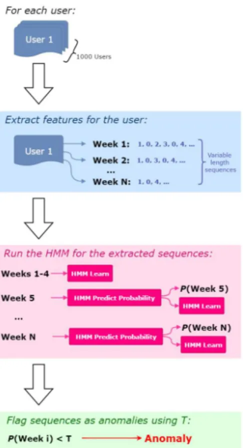
In this section we will explain the algorithms and proce-dures used for testing our model on the CERT Dataset. Fig-ure 2 shows a graphical overview of the processing approach and pipeline we use, and the remainder of this section is dedicated to describing each stage in it. The pipeline is de-signed to be very modular and thus we can easily swap out components without affecting it as a whole. For instance, we could change the features we feed into our model, or we could change our model completely without having to change the other components.
3.1
Feature Extraction
The CERT Dataset contains many log files which describe a particular kind of activity for all users (users being the same as employees), for instancehttp.csvcontains logs per-taining to web browsing (website, date accessed, username, etc.). We load each file, and assign a symbol (a number as opposed to text for convenience) to each entry based on the current set of features we are using. After this, we join all of these files, partition them by each user and then finally sort them based on the respective timestamps. For each user we get a list of actions and the time at which they undertook them. We then group these actions into weeks, which gives us the final output for the feature extraction phase: for each week we have a sequence of actions the user took. We have chosen to group based on weeks in order to allow a user’s behaviour to change throughout the week (e.g., fewer emails sent on a Friday afternoon) whilst keeping the sequence sizes
Figure 2: An overview of the pipeline we use to detect anomalies
relatively short. Experimenting with the time-scale we use is an interesting avenue of research that we have not explored in this paper, but reserve for future study. We should note that the CERT Dataset contains the ground truth for each user (when they are acting maliciously or not), which allows us to monitor the success or failure of our experiment.
3.2
Anomaly Detection
Once we have a sequence of actions that each user con-ducted in a given week, we are able to use our Hidden Markov Model (HMM). Here we introduce how the HMM is used, while Section 3.3 explains the details of the algorithms involved; understanding the these algorithms is key to ap-preciating how we look to apply HMMs to detect insiders.
To start, the HMM has 3 components which uniquely de-termine the model: the transition matrix, emission matrix and the starting state probabilities. We initialise these as being uniformly distributed with some small perturbations to break symmetry (Section 3.3.3 contains further details). We then train the model on the first 5 weeks of a user’s be-haviour in order for it to have some starting point from which to detect anomalous sequences. For the remaining weeks we first predict the probability of our model generating the se-quence, and then train the model on that sequence. The pro-cedure is described in Algorithm 1, Figure 3. HMM.Predict()
is described in Section 3.3.1, andHMM.Train()is described in Section 3.3.3.
We acknowledge that our current work makes the sig-nificant assumption that the first 5 weeks do not contain anomalous behaviour for each user. This assumption can be
Figure 3: Algorithm 1
violated for a number of reasons (short-time contractors, for instance). In the future, this could possibly be mitigated by manually checking these weeks to ensure that they are repre-sentative of normal behaviour, or, perhaps a model based on other users (roles) with similar intended behaviour could be used as the initial parameters. For now however, adopting the first 5 weeks allows us to have some basis for exploring the utility of the HMM approach to insider-threat detection. Once we have run this algorithm for all users we have the predicted probabilities for each week. We can then set a threshold T, which we use to classify sequences as anoma-lous or not. If the probability of the sequence is below the threshold, we classify it as anomalous. This thresholdTis a critical parameter of our system which must be set carefully. However, after running Algorithm 1 we can save the proba-bilities generated and then experiment with many values of
T. One could also imagine a human security analyst increas-ing Tfrom 0 in order to be presented with more instances which the system deems anomalous.
3.3
Hidden Markov Models
A Hidden Markov Model (HMM) is a Markov Model, in which the model outputs a symbol before transitioning to a new state. Figure 4 shows an ordinary Markov Model and a Hidden Markov Model. It is called a Hidden Markov Model because typically we only observe the emitted symbols, and not the states the model visited (they are hidden from us).
Figure 4: An example of a Markov Model (left) and HMM (right), with the same transition probabili-ties, but where the HMM outputs symbols {0, 1}
Below we will refer to the state the model is in at timestep
iasXi, and the symbol emitted by the model at timestepias Yi. The mechanics of the model are described via 3 distinct
quantities, which uniquely define the Hidden Markov Model:
Transition Probabilities P(Xi+1=x
′
|Xi=x) (1)
The probability of transitioning from statexto statex′
at timestepi. In order to be a Markov process we further have
the condition that: P(Xi+1=x ′ |Xi=x) =P(Xi=x ′ |Xi−1=x) (2)
This ensures that transitions are time invariant and hence only depend on the current state (this implies the Markov property). In order to be a well-defined process we also have that: ∀x∈States: X ∀x′∈States P(Xi+1=x ′ |Xi=x) = 1 (3) Emission Probabilities P(Yi=y|Xi=x) (4)
The probability of emitting symbol y, given that you are in state x at time step i. Once again we maintain time invariance to ensure the Markov property:
P(Yi=y|Xi=x) =P(Yi−1=y|Xi−1=x) (5)
At every state we must ensure the probabilities of emitting a symbol form a valid probability distribution.
∀x∈States: X
∀y∈Symbols
P(Yi=y|Xi=x) = 1 (6) Starting Probabilities
P(X0=x) (7)
The probability of the first state being statex. These must form a distribution over the set of states:
X
∀x∈States
P(X0=x) = 1 (8)
Once we have a HMM and a sequence of Symbols, there are 3 types of questions we can ask:
• What is the probability of a given observed sequence with respect to our model?
• What is the most likely sequence of states the model visited when generating a given observed sequence? • What are the parameters of our model that maximise
the probability of observing a given observed sequence? For the purposes of anomaly detection we will make use of algorithms designed to answer questions 1 and 3. Question 2 can be answered using the Viterbi Algorithm [5], but we will not make use of it in this paper.
3.3.1
Probability of an observed sequence
To calculate the probability of an observed sequenceY =
y0y1. . . yT1 with respect to our model, we partition over all
sequences of hidden states of lengtht: The probability of the first state being state x. These must form a distribution over the set of states:
P(Y) =X
X
P(Y|X)P(X) (9) whereX=x0x1. . . xT1 withxi∈States. A naive
imple-mentation calculating the sum as shown above isO(T NT)
whereN =|States|, however,P(Y) can be calculated more
efficiently using the Forward Algorithm which provides an
O(N T2) runtime.
Due to the limitations of floating point arithmetic, partic-ularly underflow, we run into significant problems when cal-culating the intermediate values for our calculations. Since all values involved are smaller than 1, they can very quickly tend to 0, which then renders subsequent calculations erro-neous due to loss of precision or even underflow to 0. To combat this we use the logarithm of the probabilities in-stead of the actual probabilities, which is standard practice used in numerical calculations involving probabilities. We thus return logP(Y) instead of P(Y). The full details of this approach for calculating logP(Y) can be referenced in Stamp [17].
3.3.2
Maximise likelihood of a sequence
The task of finding the parameters of an HMM (tran-sition, emission and starting probabilities) that maximise the likelihood of observing a given sequence can be accom-plished using the Baum-Welch Algorithm [21]. This is an iterative algorithm that improves the likelihood of a model generating a given sequence on every iteration, i.e., given
Y =y0y1...yT1 on every iteration we have that:
P(Y|θnew)P(Y|θold) (10)
whereθrepresents the parameters of our model.
However, we are not guaranteed to reach a global max-imum and in practise we are very likely to reach a local maximum which is not close to the global maximum. In addition, due to the iterative nature of the algorithm we cannot be sure if we have even reached a local maximum or not. In order to work around these problems we make use of random restarts and use thresholds to determine conver-gence (|xi+1−xi| < ǫthreshold ⇒converged). Once again
we must make concessions for floating point arithmetic, the full details of which are described in Stamp [17].
3.3.3
Training the model
Here we describe the algorithm we use to train our HMM; an overview can be seen in Figure 5. The function Baum -Welch(..) refers to running a single iteration of the
Baum-Welch algorithm on the model and sequence provided, re-turning to us the new proposed model.
Essentially the algorithm uses random restarts in order to find other maxima that are potentially better than the first one we may encounter. The parameterλ∈[0,1], which we will refer to as the inertia, is used to linearly interpo-late between the new proposed model and the old model. A higher inertia means that we will keep more of the old model. Inertia is an important parameter in our model, and as such it is important to set it correctly. We will ex-plore different values for the inertia in Section 4. It is also intended thatǫconvergence< ǫrestart. Throughout the
algo-rithm θ refers to the parameters of the model: the transi-tion, emission and starting probabilities. The function Ran-domParameters()produces random values for each quantity,
sampled uniformly from (0,1), and then normalised appro-priately to ensure valid distributions.
4.
VALIDATION
The CERT Dataset is comprised of many smaller datasets, which all represent independent logs for 1000 users over some time-framework. We have chosen to use Datasetr4.2,
Figure 5: Algorithm 2
one of these datasets, for running all of our experiments. This is because it contains many more instances of insider threats compared to the earlier datasets (70 compared to less than 4). This allows us to measure metrics such as the false-positive rate and the true-positive rate without large steps in our results (i.e., we can measure the true-positive rate in 2% or less increments compared to 33%, 50% or even 100% increments). In addition, it also provides more varied instances of attacks, since each user would exhibit their behaviour in non-identical ways. The dataset is con-sidered to be dense, with “an unrealistically high amount” (r4.2/readme.txt) of malicious activity by the creators [8]. However, this should not influence our results compared to a lighter dataset, since each user is treated independently of every other user by our system.
Reflecting on the dataset selected, there are files with user logon data, psychometric data, browsing history, file access data, email data, device usage data and LDAP data. We are provided a list of insiders for every dataset, so that we can determine our performance. The features we are using, as discussed in Section 2.2, only make use of: logon.csv,
http.csv, file.csv, email.csv and device.csv. We do not use the LDAP records orpsychometric.csv(we do not make use of a user’s psychometric scores since they do not help us to model their day-to-day behaviour directly).
As we present our results below, we make use of Receiver Operating Characteristic curves (or ROC curves). These curves are used to plot the true-positive (correct) rate against the false-positive rate for the different possible points in a diagnostic test. In order to produce the ROC curves, we use a process of threshold varying. After obtaining the log prob-abilities for each sequence from our model, we set a value for the threshold and then check each sequence one-by-one and classify them as anomalous iflogP(sequence)> T hreshold. We then increase the threshold and repeat until no sequences
are classified as anomalous. In the subsection next, we de-tail and discuss our results, and then move to consider a case study.
4.1
Results
We run Algorithm 1 as described in Section 3.2 to ob-tain our list of potential insiders. We use Algorithm 2 with the following parameters:Train(sequence, max iters= 20, ǫconvergence= 0.01, ǫrestart= 0.1,max restarts= 5,λany
value within the space [0.5,0.8])1
. For the Hidden Markov Model we use 10 states.
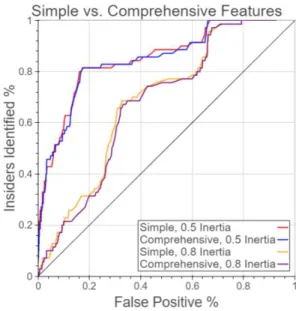
Figure 6 shows the results of running our model with those parameters. We can see that the different feature sets differ only slightly. These differences are small enough to be at-tributed to the differences introduced via the random num-ber generator running many models in parallel. The stochas-ticity of the scheduler results in the models calling the ran-dom number generator in a different order, which affects the initial initialization as well as the call toRandomParameters
in Algorithm 2. This could also be a side-effect of the syn-thetic nature of the dataset, and hence the granularity of our features could show noticeable differences in a morenatural
dataset.
Figure 6: ROC Curve showing the differences be-tween the Simple and Comprehensive feature sets for an inertia of 0.5 and 0.8
In addition to varying the feature set we use, we can also consider varying the number of states we use for our model. Figure 7 and Table 1 show the results of varying the num-ber of states in the HMM. We used the same parameters as for Figure 6 with the exception of: max iters = 50,
max restarts= 10 andλ= 0.5. We can see that increas-ing the number of states shows some slight improvements, however the computational cost of doing so (combined with increasing the number of iterations to make it viable) is ex-tremely high. Thus, we do not explore further the results of running our models with an increased number of states due to the processing time required being prohibitive for running
1
many experiments. This large computational cost is dimin-ished if our system is run in an online manner, whereby we only run it for new data points. However, for the purposes of our experiments we must run it for the entire dataset (18 months of data) every single time.
Figure 7: ROC Curve showing the difference be-tween running the model with 10, 20 and 50 states
# States Area Under Curve (AUC)
10 States 0.755
20 States 0.784
50 States 0.797
Table 1: AUC for each of the runs
An extremely important parameter in our model is the inertia, λ. In Figure 6 we saw a significant difference be-tweenλ = 0.5 and λ = 0.8. Figure 8 and Table 2 show the results of varying the inertia with the following parame-ters: Train(sequence, max iters= 20,ǫconvergence= 0.01, ǫrestart = 0.1, max restarts = 5, λ and 10 states in our
model. We can clearly see that there is a marked benefit to decreasing the inertia up till around 0.05. This is a surpris-ing result because one would expect that an inertia of 0.05 is too low to allow the model to maintain the behaviour of previous weeks.
Inertia AUC Inertia AUC
0.9 0.535 0.3 0.796 0.8 0.606 0.2 0.805 0.7 0.706 0.1 0.821 0.6 0.756 0.05 0.830 0.5 0.776 0.01 0.829 0.4 0.789
Table 2: The corresponding AUC values
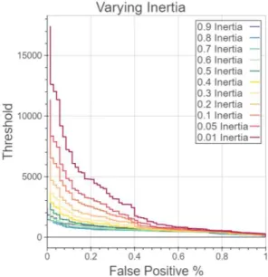
In order to investigate this further we can check the values for the threshold we use to generate each point on the ROC curve. Figure 9 shows these values for each inertia value we
Figure 8: ROC Curve showing the effect of varying the inertia in Algorithm 2
used. A higher threshold corresponds with a lower probabil-ity (i.e., in order for a sequence to be classified as anomalous, the model’s probability of generating that sequence must be lower when using a higher threshold). We observe that a lower inertia corresponds with a higher threshold for each point on the ROC curve. This implies that the values pro-duced by our HMM are more spread out with a lower inertia. We hypothesise that this decreases the effect of small vari-ances in our model’s output, and hence allows the anomalous sequences to be better separated from the other sequences.
Figure 9: The value used for the Threshold vs. False Positive % for each point on the ROC curve
Using an inertia of 0.05 shows good performance on the dataset. An AUC of 0.830 indicates we are able to success-fully identify the majority of insider threats, and in addition
the graphs show a 85% identification rate with a false posi-tive rate of only 20%. If our system was combined with more signals of insider attacks (as in [1]), as well as more tradi-tional security monitoring tools (e.g., flag up visits to certain websites), we hypothesise that potentially much better per-formance could be achieved. We believe that incorporating other approaches would provide complimentary indicators of an insider threat. This is because our approach is de-signed to capture deviations from a user’s normal behaviour, whereas those other approaches capture other separate in-dicators of an attack.
4.2
Case Study
Dataset r4.2 contains 70 malicious insiders who execute one of three attacks. Now, we consider a brief case study with a single insider, User MCF0600, in more detail so that we can better understand how and why our model correctly classifies them as a threat. The attack carried out by this user is as follows: User MCF0600 begins to logon after hours, starts using a removable drive and then begins uploading data towikileaks.org.
We will use the Simple feature set to simplify our visualisa-tion, and run the model with 10 states and the following pa-rameters: Train(sequence, max iters= 20, ǫconvergence =
0.01, ǫrestart= 0.1,max restarts= 5,λ= 0.05. Figure 10
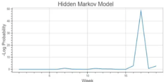
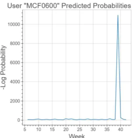
shows the model’s probability of generating each week’s ac-tivities. We see a large spike at Week 39 which corresponds to the dates 20/9/2010 till 26/9/2010 in the dataset. This is the exact week which contains the malicious behaviour in which the user attacks the company by uploading data to wikileaks.org.
Figure 10: User MCF0600’s predicted probabilities for each week
Figure 11 shows a visualisation of the model at Week 38, which is used to predict the likelihood of the actions taking place in Week 39. It shows the model learns the user frequently visits websites, and occasionally sends emails throughout the day. Notably there is an absence of remov-able drive usage and the downloading of files. In detail, the Starting probabilities for each state are concentrated on State 9 (P(X0 = State9) = 1), represented by the purple
arrow. Similarly, the emission probabilities for each state are concentrated on a single symbol, hence only that sym-bol is shown for each state. The transition probabilities are more varied, hence we only show those>0.2 otherwise the
diagram quickly becomes too noisy. Note that State 5 is not shown in the diagram, because there is no significant prob-ability (>0.2) of transitioning to it from any other state.
Figure 11: The Hidden Markov Model after week 38 for User MCF0600
More generally, a sample from the first day of the week with malicious activity is:
[‘Logon’, ‘Connect’,‘File’, ‘Disconnect’, ‘Connect’, ‘File’, ‘File’, ‘File’, ‘Disconnect’,. . .].
It is clear that this does not conform to the user’s normal behaviour due to the marked increased usage of a removable drive, and the downloading of files. Contrast this sequence with another normal day for this user which is modelled al-most perfectly by the model:
[‘Logon’; ‘Website’; ‘Website’; ‘Website’; ‘Email’; [‘ Web-site’×7]; ‘Logoff’]
From our case study we see promising indicators that our model effectivelylearnsa user’s behaviour, and then can ac-curately use that to determine deviations from it. We should note that it is the features identified from our literature re-view to be characteristic of insider threats that enable the HMM algorithms to flag anomalies relevant to insider activ-ities. Therefore, a deeper understanding of how insiders act and which characteristics can be identified in their malicious activities is of significant importance for our detection sys-tem since they can more accurately profile the behaviour of an insider. For the needs of the CERT case study and given the limited number of different types of logs in the dataset, we emphasised in providing features for detecting suspicious activity related to intellectual property theft.
5.
CONCLUSIONS
In this paper we have examined the problem of insider threat detection, by framing it as a machine learning task. Our main contribution is the development and testing of a novel method of using Hidden Markov Models to learn a user’s normal behaviour in order to identify deviations from it, which may be indicative of a threat (or at least behaviour worth following-up).
From our results we can see that our system is able to detect insider threats with a reasonable false-positive rate. Furthermore, our case study of user MCF0600 shows that the HMM is able to learn a user’s behaviour and determine when the user deviates from that behaviour. In addition, the use of a HMM allows us to visualise the model, and thus
to determine what the model deems as normal behaviour which allows us to understand why a particular sequence of actions is classified as anomalous. This is extremely perti-nent information, since there are severe repercussions when an employee is flagged as a potential threat to an organisa-tion. By allowing a human security analyst the chance to investigate the offending behaviour we can provide valuable insight into why an attack took place, and also to allow false positives to be identified as such.
5.1
Limitations
In the exploration into the utility of HMM to insider-threat detection, we have made many assumptions that could limit the effectiveness of our approach in certain scenarios. We enumerate the most important of these, and the possible effect they could have on our system below.
Insider attacks are anomalous: The most significant assumption we have made is that all insider attacks are ex-amples of anomalous behaviour. This precludes us from recognising situations where a user systematically attacks an organisation over an extended time-framework (e.g., down-loading sensitive files over months), or situations where our features are not sufficient to distinguish an attack from a user’s normal behaviour.
Training on the first 5 weeks: In order to apply our model, we must first ensure that it is able to distinguish a user’s normal behaviour from anomalous behaviour. This then means that we must train on some sample of a user’s behaviour in order for the model to learn normal behaviour. Hence we are not looking for insider threats in that training set, which in our specific case means that we do not consider that a user might attack in the first 5 weeks. This could significantly hamper our ability to detect insider threats amongst short-term users (contractors for instance), which are a real threat [11].
Features: Our approach is only able to make use of the information that it is provided, and hence depends on the features that it is supplied with. This requires domain knowledge and manual feature engineering and experimen-tation in order to produce useful features. Our approach would therefore need to be adapted somewhat depending on application cases.
Choosing Hyperparameters: As is the case with many machine learning systems, our approach involves many dif-ferent hyperparameters which must be set. Our results show that some of these (the inertiaλparticularly) have a signifi-cant effect on the final results of the model, and hence these must be chosen carefully. This could lead to decreased per-formance on a real dataset where we would not have the benefit of knowinga priori who the insiders are. However, the hyperparameters can be changed whilst running the sys-tem, or we can initialise them based on results from other datasets.
5.2
Future Research
Our modular approach to the design of our systems means that each of the components could be replaced without af-fecting the others. This allows us to make changes to each of the individual parts without re-thinking the entire sys-tem. As this paper aimed to explore the utility of HMMs to detect insidrer threats, we discuss some areas that would be interesting for follow-on research below.
In our approach we have grouped a user’s actions into
week long sequences. Experimenting with different time-frameworks, such as day long sequences, could provide better performance. Using shorter sequences could allow specific events to be pinpointed as the source of concern, and could also allow the model to build a more accurate picture of a user’s day-to-day behaviour. However, it could also prevent the model from observing longer-term trends in behaviour (e.g., on Friday a user sends fewer emails), so would have to be properly considered.
We have focussed on using a HMM for the task of learning a user’s behaviour and then outputting how likely a partic-ular sequence of actions is with respect to the user’s past behaviour. We could replace the HMM with a more com-plex model such as a Long Short-Term Memory Recurrent Neural Network (LSTM) [7], in order to learn a richer rep-resentation of a user’s behaviour. A LSTM does not make the Markov assumption, and hence is able to use longer-term dependencies in order make a more informed decision about the current action a user might take. This could stem from the inability of a HMM to use many bits of informa-tion about the past, without an exponentially large number of states (a HMM needs around 2kstates to modelkbits of information), whereas a LSTM can make use of potentially all the information it has seen. However, a LSTM could re-quire significantly more training data in order to be effective; as with all techniques there are pros and cons.
Our current procedure for determining if a particular se-quence is anomalous or not is to compare the probability of our model generating it with a threshold. This requires us to manually set a threshold value, which is another hyperpa-rameter of our system that significantly affects the results. However, we could consider the task of determining which sequence is anomalous with respect to their probabilities as an anomaly detection problem itself. Hence, we could apply frequency-based anomaly detection techniques (e.g., [19]) on the sequences of probabilities generated by our model. This allows us to avoid having to manually set a threshold pa-rameter, and also allows us to be more selective in flagging up sequences as anomalous. Moreover, it could help in the case where our model is unable to determine a user’s normal behaviour accurately (or if the user’s behaviour is erratic). Since in this scenario the majority of sequences will be un-likely with respect to the model, we would only want to classify as anomalous those as that are significantly more unlikely.
6.
REFERENCES
[1] O. Brdiczka, J. Liu, B. Price, J. Shen, A. Patil, R. Chow, E. Bart, and N. Ducheneaut. Proactive insider threat detection through graph learning and psychological context. InIEEE Security and Privacy Workshops, 2012. DOI: 10.1109/SPW.2012.29. [2] D. M. Cappelli, A. P. Moore, and R. F. Trzeciak.The
CERT Guide to Insider Threats: How to Prevent, Detect, and Respond to Information Technology Crimes. Addison-Wesley Professional, 1st edition, 2012.
[3] Y. Chen and B. Malin. Detection of anomalous insiders in collaborative environments via relational analysis of access logs. InProceedings of the first ACM conference on Data and application security and privacy, pages 63–74. ACM, 2011.
[4] Department of Homeland Security (DHS). Combating the insider threat, 2014.
https://www.us-cert.gov/sites/default/files/publications/Combating the Insider Threat 0.pdf.
[5] G. D. Forney. The viterbi algorithm.Proceedings of the IEEE, 61(3):268–278, 1973.
[6] Gemalto. Breach level index|data breach database & risk assessment calculator, 2016.
http://www.breachlevelindex.com/.
[7] S. Hochreiter and J. Schmidhuber. Long short-term memory.Neural computation, 9(8):1735–1780, 1997. [8] Insider Threat Tools – The CERT Division, n.d.
https://www.cert.org/insider-threat/tools/.
[9] Y. Liao and V. R. Vemuri. Use of k-nearest neighbor classifier for intrusion detection.Computers & Security, 21(5):439–448, 2002.
[10] C. C. Michael and A. Ghosh. Two state-based approaches to program-based anomaly detection. In
Computer Security Applications, 2000. ACSAC’00. 16th Annual Conference, pages 21–30. IEEE, 2000. [11] J. R. C. Nurse, O. Buckley, P. A. Legg, M. Goldsmith,
S. Creese, G. R. Wright, and M. Whitty. Understanding insider threat: A framework for characterising attacks. InIEEE Security and Privacy Workshops (SPW). IEEE, 2014. DOI:
10.1109/SPW.2014.38.
[12] P. Parveen, N. McDaniel, V. S. Hariharan, B. Thuraisingham, and L. Khan. Unsupervised ensemble based learning for insider threat detection. InPrivacy, Security, Risk and Trust (PASSAT), 2012 International Conference on and 2012 International Confernece on Social Computing (SocialCom), pages 718–727. IEEE, 2012.
[13] P. Parveen and B. Thuraisingham. Unsupervised incremental sequence learning for insider threat detection. InIntelligence and Security Informatics (ISI), 2012 IEEE International Conference on, pages 141–143. IEEE, 2012.
[14] Ponemon Institute. 2015 Cost of Cyber Crime Study, 2015.
http://www8.hp.com/uk/en/software-solutions/ponemon-cyber-security-report/.
[15] L. R. Rabiner. A tutorial on hidden markov models and selected applications in speech recognition.
Proceedings of the IEEE, 77(2):257–286, 1989. [16] B. Sch¨olkopf, J. C. Platt, J. Shawe-Taylor, A. J.
Smola, and R. C. Williamson. Estimating the support of a high-dimensional distribution.Neural
computation, 13(7):1443–1471, 2001.
[17] M. Stamp. A revealing introduction to Hidden Markov models (San Jose State University), 2015.
http://www.cs.sjsu.edu/faculty/stamp/RUA/HMM.pdf. [18] E. Ted, H. G. Goldberg, A. Memory, W. T. Young,
B. Rees, R. Pierce, D. Huang, M. Reardon, D. A. Bader, E. Chow, et al. Detecting insider threats in a real corporate database of computer usage activity. In
Proceedings of the 19th ACM SIGKDD international conference on Knowledge discovery and data mining, pages 1393–1401. ACM, 2013.
[19] O. Vallis, J. Hochenbaum, and A. Kejariwal. A novel technique for long-term anomaly detection in the cloud. In6th USENIX Workshop on Hot Topics in Cloud Computing, 2014.
[20] C. Warrender, S. Forrest, and B. Pearlmutter. Detecting intrusions using system calls: Alternative data models. InSecurity and Privacy, 1999. Proceedings of the 1999 IEEE Symposium on, pages 133–145. IEEE, 1999.
[21] L. R. Welch. Hidden Markov Models and the Baum-Welch Algorithm.IEEE Information Theory Society Newsletter, 53(4), 2003.
[22] K. Xu, D. D. Yao, B. G. Ryder, and K. Tian. Probabilistic program modeling for high-precision anomaly classification. In2015 IEEE 28th Computer Security Foundations Symposium, pages 497–511. IEEE, 2015.