Discriminative Elastic-Net Regularized Linear
Regression
Zheng Zhang, Zhihui Lai, Yong Xu,
Senior Member, IEEE,
Ling Shao,
Senior Member, IEEE,
Jian Wu, Guosen Xie
Abstract—In this paper, we aim at learning compact and discriminative linear regression models. Linear regression has been widely used in different problems. However, most of the existing linear regression methods exploit the conventional zero-one matrix as the regression targets, which greatly narrows the flexibility of the regression model. Another major limitation of theses methods is that the learned projection matrix fails to precisely project the image features to the target space due to their weak discriminative capability. To this end, we present an elastic-net regularized linear regression (ENLR) framework, and develop two robust linear regression models which possess the following special characteristics. First, our methods exploit two particular strategies to enlarge the margins of different classes by relaxing the strict binary targets into a more feasible variable matrix. Second, a robust elastic-net regularization of singular values is introduced to enhance the compactness and effectiveness of the learned projection matrix. Third, the resulting optimization problem of ENLR has a closed-form solution in each iteration, which can be solved efficiently. Finally, rather than directly exploiting the projection matrix for recognition, our methods employ the transformed features as the new discriminate representations to make final image classification. Compared with the traditional linear regression model and some of its variants, our method is much more accurate in image classification. Extensive experiments conducted on publicly available datasets well demonstrate that the proposed framework can outperform the state-of-the-art methods. The MATLAB codes of our methods can be available at http://www.yongxu.org/lunwen.html.
Index Terms—Elastic-Net regularization, discriminative meth-ods, linear regression, image classification
I. INTRODUCTION
D
ISCRIMINATIVE methods (e.g., regression models) have a good reputation in both theoretical research and practical applications, and also have been extensively applied to solving many computer vision problems [1], [2]. Different from the probabilistic models, discriminative meth-ods typically project image features to some continuous orManuscript received *** **, 2016; revised *** **, 2016; accepted *** **, 2017. This work was supported by the National Natural Science Foundation of China under Grant 61370163, and Grant 61233011. (Corresponding author:
Yong Xu.)
Z. Zhang, Y. Xu and J. Wu are with the Bio-Computing Research Center, Shenzhen Graduate School, Harbin Institute of Technology, Shen-zhen 518055, China (e-mail:[email protected], [email protected], [email protected]).
Z. Lai is with the College of Computer Science and Software Engineering, Shenzhen University, Shenzhen 518055, China, and also with the Institute of Textiles&Clothing, Hong Kong Polytechnic University, Hong Kong (e-mail: lai zhi [email protected]).
L. Shao is with the School of Computing Sciences, University of East Anglia, Norwich NR4 7TJ, U.K. (e-mail: [email protected]).
G. Xie is with the Department of Information Engineering, Henan Univer-sity of Science and Technology (e-mail: [email protected]).
discrete targets, and then exploit the projection matrix to make image classification or regression [3], [4]. In addition, discriminative methods can achieve impressive performance when constructing robust projection matrix and providing sufficient training samples [5], [6]. However, the problem of robust discriminative learning has not been exhaustively explored and perfectly solved.
Least square regression (LSR) is a typical and fundamen-tal technique in statistics theory. Due to its mathematically tractable and efficient solution as well as simple yet effec-tive formulation, LSR has been widely used in many other applications such as computer vision and pattern recognition [7]. Many variations have been proposed to enhance the performance of the conventional LSR, such as partial LSR [8], weighted LSR [9], and nonnegative least squares [10]. Moreover, extensive discriminative LSR methods have been developed to improve the robustness and effectiveness of the existing regression approaches. For example, Xiang et al. [7] designed a general framework of discriminative least square regression (DLSR) by introducing the ε-dragging technique for image classification and feature selection, and Zhang et al. [11] introduced a method of retargeted LSR by learning transformed regression. A unified least square framework [12] is constructed to formulate many component analysis methods and generate their regularized and kernel extensions. Thus, LSR model has become a popular technique and also has been widely adopted to deal with recognition and classification tasks [13].
Another important and fundamental variant of LSR is the problem of least absolute shrinkage and selection operator, i.e. LASSO [14], or sparse representation problem [6], [15]. Sparse representation based classification (SRC) method [15] has been extensively applied to addressing the face recognition problem, and the performance is very impressive. Subse-quently, numerous representation based classification methods have been proposed to improve its effectiveness, robustness and efficiency of face recognition [16]. For example, linear regression based classification (LRC) [17] method exploits the linear combination of each class of training samples to represent the test sample, and then classifies the test sample to the class which leads to the minimum representation residual. Collaborative representation based classification method (CR-C) [18] introduces thel2-norm regularization instead of the l1-norm regularization for efficient face recognition. Specifically, literature [18] demonstrates that SRC theoretically is a special case of the collaborative representation method, and the com-putational efficiency of CRC is dramatically higher than SRC
without sacrificing much classification accuracies. Moreover, locality-constrained linear coding (LLC) enforces the locality constraints to perform a local embedding of the descriptors [19], [20]. In addition, the representation based technique has been introduced to a wide range of applications.
The low-rank minimization problem has attracted a lot of attention due to its effectiveness on data representation [21]. It is worth noting that robust PCA (RPCA) [22] is one of the most popular methods based on the low-rank minimization. Providing that data are lying in a single subspace, RPCA decomposes the observed data into two components, the rank uncorrupted data term and sparse noise term. The low-rank regression model [23] has been studied because of the apparent advantage of the low-rank characteristics [22], [24], [25]. Based on the traditional low-rank linear regression (L-RLR) model, Cai et al. [23] proposed two low-rank regression models, i.e. rank ridge regression (LRRR) and sparse rank regression (SLRR) methods. Specifically, these three low-rank regression models are equivalent to linear discriminant analysis based regressions [23]. Furthermore, all of them are based on the nature of the low-rank minimization, which can capture the underlying structure of data correlation patterns [22], [24]. Latent low-rank representation (LatLRR) [26] ex-plores the unobserved hidden information of data, and can robustly extract salient features from noise or corrupted data. Subsequently, many variations of the low-rank minimization have been applied to solve different problems [3], [27]– [29]. For example, Li and Fu [3] proposed a supervised regularization-based robust subspace learning method by joint-ly removing noise term with low-rank constraint and learning a discriminate subspace from the clean data. Wei et al. [27] designed a method of low-rank matrix recovery method by embedding the structure incoherence (LRSI) information for robust face recognition. Li et al. [28] constructed a classwise block-diagonal structure (CBDS) dictionary by imposing the class-wise discriminative structure regularization term to make the samples from different classes be reconstructed with d-ifferent bases. Benefiting from recent advances on low-rank minimization, a framework of robust regression model [2] was proposed to solve several computer vision problems.
Nonetheless, most existing regression methods in the learn-ing phase only focus on directly projectlearn-ing the original visual features to conventional zero-one target matrix, which pro-vides too little freedom to fit the strict binary label matrix. Moreover, the projection matrices learned by these methods fail to precisely project the image features to the target fields due to its weak discriminative capability. It is notable that a robust and discriminative regression method should equip with three-fold characteristics, i.e. compact projection matrix, discriminative regression targets and robust to errors in the data. Given these deficiencies, this paper develops a novel elastic-net regularized linear regression (ENLR) framework, and two robust ENLR methods, i.e. discriminative ENLR and marginalized ENLR, are proposed to construct a robust and compact regression model for multi-category image classifi-cation. More specifically, the elastic-net regularization term is accumulated to learn a more compact projection matrix, and at the same time, enlarging the margins of different classes is
significant and beneficial to the classification tasks. Based on theε-dragging technique, the discriminative regression targets are further formulated to better fit regression tasks. Moreover, marginalized regression targets are learned directly from data by enforcing a strong constraint on the learned targets between the true and false classes. Furthermore, instead of directly exploiting the projection matrix for classification, the data points under the simple linear transformation using the learned projection matrix are employed to final classification such that the transformed data is more discriminative and robust to errors. In addition, the low-rank model always suffers from heavy computational burden due to singular value decomposi-tion procedure. To efficiently solve it, ENLR introduces an al-ternative definition of the nuclear-norm with a strong convexity strategy such that our method can be scalable to large data sets. To the best of our knowledge, this is for the first time to unify the elastic-net regularization of singular values and learning discriminative regression targets into one framework, which is a very simple but extraordinarily effective method for image classification. The effectiveness of the ENLR framework is demonstrated on different classification tasks. Therefore, the main contributions of this paper are summarized as follows.
(1) In this paper, the elastic-net regularization of singular values and constructing distinctive regression targets are for the first time integrated into one unified discriminative lin-ear regression framework. The underlying characteristics of the elastic-net regularization of singular values are explicitly uncovered and analyzed such that the elastic-net theory is extended to the elastic-net regularization of singular values.
(2) By virtue of enlarging the margins of different classes, we propose two robust elastic-net regularized linear regression methods as well as the corresponding alternative efficient methods. Specifically, the discriminative ENLR (DENLR) method interpolates the ε-dragging technique into the ENLR framework, and a more flexible marginalized ENLR (MENLR) method is developed by directly learning the marginal regres-sion targets from data, in which a strong marginalized con-straint is enforced to make the learned targets distinguishable. (3) Two efficient algorithms are proposed to solve the result-ing optimization problems, and theoretical and experimental analysis are conducted to prove the convexity and convergence of the designed optimization algorithms. Additionally, the the-oretical relationships between the proposed ENLR framework and the prevailing LSR models are revealed.
The rest of this paper is organized as follows. We briefly introduce some related works in Section II. Then, we describe the proposed ENLR framework and theoretical analysis in Section III, and optimization algorithm is presented in Section IV. Extensive experiments are reported in Section V. Finally, the conclusion remarks and our future work are summarized in Section VI.
II. RELATEDWORK A. Notation
The matrix is denoted by bold uppercase letters, e.g.X, and thei-th row andj-th column element of matrixX is denoted asXij. Column vectors are denoted by bold lower letters, e.g.
x.∥X∥2
F =tr(X
TX) =tr(XXT)designates the Frobenius
norm of matrix X, where tr(•) is the trace operator. ∥X∥∗
is the nuclear norm of the matrix X, i.e. ∥X∥∗ = ∑i|σi|
whereσi is thei-th singular value of matrixX.XT denotes
the transposed matrix of X andI denotes an identity matrix.
B. Linear regression model
Linear and non-linear regression have been widely applied to many computer vision problems, such as classification [2], [7], [11]. Standard linear regression model for classifi-cation is to learn a linear projection matrix in the training stage, and uses it to project the observed image features
X = [x1,· · ·, xn]∈ ℜd×n approximate to the target matrix
Y = [y1,· · ·, yn]T ∈ ℜn×c by minimizing
min
D ∥X
TD−Y∥2
F, (1)
where X is the given data set, D ∈ ℜd×c is the learned projection matrix, and Y is the corresponding binary class indicator matrix. Specifically, yi ∈ ℜc is the label vector of
thei-th samplexi, andnandcare the number of samples and
classes, respectively. A more popular-used regularized linear regression model is formulated by addressing the following optimization problem
min
D,b∥X
TD+enbT−Y∥2
F +λ∥D∥2F. (2)
The general steps of the linear regression model for image classification task are as follows. In the training stage, we learn the projection matrix D, and any test point is estimated by DTxte in the test step.
C. Low-rank linear regression model
The low-rank linear regression (LRLR) model [23] is a modified version of the standard linear regression model (1). Compared to the conventional linear regression model, a more compact low-rank projection is learned by enforcing the rank minimization constraint to explore the underlying correlation structures between classes [23], and the objective function of LRLR is formulated as
min
D ∥X
TD−Y∥2
F+λrank(D). (3)
Because of the discrete property of the rank function, which is a non-convex non-smooth problem, a tractable optimization problem is reformulated by replacing the rank function with the nuclear norm regularization [32], i.e.
min
D ∥X
TD−Y∥2
F+λ∥D∥∗. (4)
The nuclear norm regularization can effectively discover the hidden structures between classes such that the learned low-rank projection matrix is more compact and discriminative than the traditional projection matrix. The low-rank linear regression model is demonstrated to be equivalent to the linear discriminant analysis based regression [23]. It is worth noting that the low-rank linear regression models can provide better data mining results in comparison with the existing full-rank linear regression models [23].
III. THE PROPOSEDENLRFRAMEWORK
In this section, we focus on learning a compact and dis-criminative regression model for robust multi-category image classification. For linear regression model, compact projection matrix and discriminative regression targets are both impor-tant. We introduce an elastic-net regularization of singular values term to formulate robust projection matrix, and the enlarged slack regression targets are constructed to improve its discriminant. Therefore, an elastic-net regularized linear regression (ENLR) framework and two discriminative linear regression methods are proposed for image classification.
A. A general framework of elastic-net regularized linear re-gression model
To learn a compact and discriminative projection matrix, a general framework of elastic-net regularization based linear regression model is formulated as
min D ϕ(D) +λ1∥D∥∗+ λ2 2 ∥D∥ 2 F, (5)
whereλ1andλ2are the regularization parameters for balanc-ing respective terms. The most straightforward regression loss function isϕ(D) =∥XTD−Y∥2F. For the above objective function (5), we have the following proposition.
Proposition 1:Objective function (5) is a robust regression problem with an elastic-net regularization of singular values.
The singular value decomposition (SVD) factorizes the linear transformation matrixDinto
D=UΣVT =
r
∑
i=1
uiσivTi , (6)
wherer= min{c, d}is the rank of D,ui∈ ℜd andvi ∈ ℜc
are respectively the left and right singular vectors ofD, and
σi is the i-th singular value of matrix D.
It is notable that the nuclear norm of matrix D can be interpreted as a sum of the singular values, i.e. ∥D∥∗ =
∑r
i|σi|, and the Frobenius norm of matrix D is ∥D∥2F =
tr(DDT) = tr(UΣVTVΣUT) = tr(Σ2) = ∑i|σi|2.
Thus, by integrating the nuclear norm and the Frobenius norm penalties of matrixD, we have the elastic-net regularization of singular values term, i.e.∥D∥∗+∥D∥F2 =∑i|σi|+
∑
i|σi|2.
Typically, the large singular values always highlight the components where the fundamental information lies. It is interesting to note that the singular values can directly reflect the importance of underlying components of data. For exam-ple, smaller singular values always come from the redundant or noise-contaminated components when the data contains redundant information or noise. It seems natural to use the measurement of singular values to analyze data. Based on these observations, the elastic-net regularization of singular values provides an advisable approach to removing the redun-dant components based on the following proposition.
Proposition 2: The elastic-net regularization of singular values can effectively enable automatic grouped variable s-election of principal components and continuous shrinkage of redundant components.
Based on Proposition 1, we know that the elastic-net reg-ularization of singular values is composed of the l2-norm and l1-norm regularization of singular values. It is known that the l2-norm regularization of singular values tends to shrink a variable towards zero but generally keeps all the components in the model, which may lead to redundant information in predictors. However, this deficiency of the l2-norm regularization fortunately generates the grouping charac-teristic in the model-fitting procedure. On the contrary, the l1-norm regularization of singular values can produce automatic selection of principal information and continuous shrinkage of redundant information simultaneously [14]. However, one significant limitation of thel1-norm regularization is that when the correlations among a group of variables are very high, it tends to select only one variable from the group, but neglects the remaining ones, which may lead to sub-optimal results. The feasible way of overcoming this deficiency is to regard the highly-correlated group as a whole to make variable selection, i.e. grouped variable selection. Therefore, it is reasonable to mix thel2-norm andl1-norm regularization of singular values, yielding the elastic-net regularization of singular values, which can effectively enable automatic grouped variable selection of principal components and continuous elimination of depen-dencies and redundancies in data. In this way, the proposed ENLR framework is a succinct and stable linear regression formulation.
Furthermore, given optimal regression D, we will project
x to the target space (e.g. label space) by
DTx= ´ r ∑ i=1 σi(uTix)vi, (7)
wherer´is the number of selected singular values. Herein the target space can be viewed as a weighted linear combination of target-component vectors {vi}´ri=1, and the i-th weight is composed of two terms, i.e. the i-th singular value σi,
and transformed feature value uTix, which is determined by the feature-component vectors {ui}´ri=1. We can see that the optimized selection of singular values can generate the optimal feature-component and target-component vectors such that the importance of the feature correlations and target correlations is simultaneously uncovered.
Moreover, the elastic-net regularization of features has shown its great superiorities in comparison with the ridge regularization [18] and LASSO [14] in many applications such as feature selection [33] and matrix factorization [30]. However, the elastic-net regularization of features can not effectively capture and mine the subtle information from data, whereas exploiting the elastic-net regularization of singular values can attain a more compact and distinctive projection matrix, which improves the performances of linear regression models. Based on the elastic-net regularized linear regression framework in Eq. (5), two robust elastic-net regularized linear regression methods are proposed, i.e. discriminative elastic-net regularized linear regression (DENLR) and marginalized elastic-net regularized linear regression (MENLR).
B. Discriminative Elastic-net Regularized Linear Regression
To enhance the discriminative capability of regression re-sults, the ε-dragging technique is introduced to transform the strict zero-one regression targets into the disjunctive but discriminative ones such that the regression model is more robust. Due to the weak separability of the strict binary regression targets in (1), theε-dragging technique enforces the regression targets of different classes moving along mutual opposite directions such that the margins between different classes are enlarged and more discriminative regression targets are achieved.
We take an example to introduce the rationale of the ε-dragging technique and demonstrate that the reformulated regression targets are more discriminative than Y. Let x1, x2, x3 be three training samples, which are respectively from the third, first and second classes, and then the corresponding binary-class label matrix is defined as
Y =
01 00 10 0 1 0
∈ ℜ3×3. However, we expect that the strict binary regression target matrix can be relaxed into some soft extent to fit the data. To this end, a slack variable matrix is constructed by using the ε-dragging technique, which drags these binary outputs far way along different directions. More specifically, if we take the above three samples as an example, the regression target matrix is defined as Y˜ = 1 +−m11m21 −−m12m22 1 +−m23m13 −m31 1 +m32 −m33 , s.t. mij ≥0.
Apparently, the distance of each sample in matrix Y is √2, while the distance between each sample inY˜ is bigger than or equal to√2owing to the nonnegative constraint of parameter ms. For example, the first and second sample in Y˜ is
√
(−m11−1−m21)2+ (−m12+m22)2+ (1 +m13+m23)
≥ √2. It is easy to see that the margins of the different classes are enlarged.
By introducing the ε-dragging technique, a discriminative elastic-net regularized linear regression (DENLR) model is developed, and its objective function is formulated as
min D ψ(D) +λ1∥D∥∗+ λ2 2 ∥D∥ 2 F, (8) where ψ(D) = ∥XTD − Y˜∥2
F and Y˜ is the relaxed
regression target matrix.
To obtain an optimalY˜, an elaborate strategy is devised as follows. LetEbe a constant matrix, and thei-th row andj-th column entry is defined as
Eij=
{
+1 if Yij = 1
−1 if Yij = 0,
(9) and then, we have Y˜ = Y +E ⊙M, where M ∈ ℜn×c
is a learned nonnegative matrix. Thus, the proposed DENLR model (8) is rewritten as the following optimization problem:
min D,M∥X TD−(Y +E⊙M)∥2 F+λ1∥D∥∗ +λ2 2 ∥D∥ 2 F s.t. M ≥0. (10)
C. Marginalized Elastic-net Regularized Linear Regression
From problem (10), we can see that the relaxed target space of DENLR is subject to the bound that the regression results should be larger than 1for true classes and smaller than0 for false classes. However, this target space is still based on the zero-one label matrixY, which greatly confines the flexibility of the regression model. To this end, we propose to directly learn the regression targets from data, and a marginalized con-straint is enforced to make the learned targets distinguishable. We consider the following marginalized elastic-net regularized linear regression (MENLR) problem:
min D,R∥X TD−R∥2 F+λ1∥D∥∗+ λ2 2 ∥D∥ 2 F s.t. riyi−max j̸=yirij ≥C, i= 1,· · ·, n, (11)
where R = [r1,· · ·,rn]T ∈ ℜn×c is the learned regression
targets, and C is a constant. Herein yi denotes the index of
the true class for thei-th samplexi. That is, if thei-th sample
is from the m-th class (i.e. yi=m), the value of the m-th
element of the learned target vector ri, i.e. rim, should be
bigger than the rest of the elements by a fixed margin of C. Similar to SVM [43], we simply set the marginal value between the true and the false classes to 1, i.e. C = 1. Apparently, the marginalized constraint makes the learned regression targets between the true and false classes separable by a fixed distance such that the proposed MENLR is more flexible and discriminative.
D. Efficient ENLR
For large-scale image classification tasks, the computation complexity of the designed model should be seriously taken into consideration. Thus, the following theorem [34] can make our models appropriate for practical applications.
Theorem 1. For any matrixD, we have the following equa-tion: ∥D∥∗= min D=AB∥A∥F∥B∥F = minD=AB 1 2(∥A∥ 2 F+∥B∥ 2 F). (12)
Proof. For better flow of the paper, we move the proof of Theorem 1 to Appendix A.
Based on the Theorem 1, we make an equivalent represen-tation of DENLR as min D,M,A,B∥X TD−(Y +E⊙M)∥2 F+ λ1 2 (∥A∥ 2 F +∥B∥2F) +λ2 2 ∥D∥ 2 F s.t. D=AB, M ≥0, (13)
and MENLR is rewritten as min D,R∥X TD−R∥2 F + λ1 2 (∥A∥ 2 F+∥B∥ 2 F) +λ2 2 ∥D∥ 2 F s.t. D=AB,riyi−max j̸=yi rij ≥C. (14)
IV. OPTIMIZATION ANDALGORITHMANALYSIS
In this section, we present two efficient and effective opti-mization algorithms to solve (13) and (14). In general, the two optimization problems with the low-rank constraintD=AB
are both non-convex and non-smooth problems. Fortunately, ALM provides a preferable way to find minimum points of such optimization problems with equality constraints as (13) and (14). To obtain efficient solutions, we utilize the ALM strategy to optimize the resulting problems in an alternative minimization manner, i.e. minimizing the loss with respect to one variable when fixing the rest variables [35].
A. Optimization of DENLR
The ALM strategy solves the problems by alternatively minimizing the augmented Lagrangian of the original prob-lems and maximizing the dual probprob-lems. Here the augmented Lagrangian function of problem (13) is
L(D,M,A,B,C1) =∥XTD−(Y +E⊙M)∥2F+ λ2 2 ∥D∥ 2 F +λ1 2 (∥A∥ 2 F+∥B∥2F) +⟨C1,D−AB⟩+ µ 2∥D−AB∥ 2 F, (15) where ⟨P,Q⟩=tr(PTQ), C
1 is a Lagrange multiplier and µ >0is a penalty parameter. The minimum points of Lwith respect to primal variables can be found via the block coor-dinate descend (BCD) method. The augmented Lagrangian is minimized along one coordinate direction at each iteration. We expand this procedure in more details.
Updating A: Fix the other variables and update A by solving the following problem.
A+ = arg min A λ1 2 ∥A∥ 2 F+<C1,D−AB>+ µ 2∥D−AB∥ 2 F = arg min A λ1 2 ∥A∥ 2 F + µ 2∥D−AB+ C1 µ ∥ 2 F, (16) where the rest terms irrelevant to AinL are viewed as con-stants and ignored in the loss since they make no differences in this particular procedure. The resulting problem (16) is a typical regularized least square problem, hence its solution is easily obtained as
A+= (C1+µD)BT(λ1I+µBBT)−1. (17)
Updating B: The variable B plays a symmetric role to that of A in L, hence the updating of B is performed in a symmetric way: B+= arg min B λ1 2 ∥B∥ 2 F+⟨C1,D−AB⟩+ µ 2∥D−AB∥ 2 F = arg min B λ1 2 ∥B∥ 2 F+ µ 2∥D−AB+ C1 µ ∥ 2 F. (18) Similarly, B+ = (λ1I+µATA)−1AT(C1+µD). (19)
Algorithm 1.Optimization of DENLR by Exact ALM Require:Feature Matrix X; Label MatrixY; Constant matrix
E; Parametersλ1,λ2.
Initialization:M =0,D∈ ℜd×c,A∈ ℜd×r,B∈ ℜr×c,
C1∈ ℜd×c,λ1>0,λ2>0,µ >0.
Whilenot convergeddo Whilenot convergeddo
Step 1. UpdateAby solving problem (16); Step 2. UpdateBby solving problem (18); Step 3. UpdateDby solving problem (20); Step 4. UpdateMby solving problem (22); End While
Step 5. Update the Lagrange multipliersC1by
C1=C1+µ(D−AB).
End While
Output:Projection matrixDˆ
Updating D: Fix the other variables and update D by solving the following problem.
D+= arg min D ∥X TD−S∥2 F+ λ2 2 ∥D∥ 2 F +⟨C1,D−AB⟩+ µ 2∥D−AB∥ 2 F = arg min D ∥X TD−S∥2 F+ λ2 2 ∥D∥ 2 F +µ 2∥D−AB+ C1 µ ∥ 2 F, (20)
whereS =Y +E⊙M. By setting the derivative ∂∂DL =0, we can infer the optimal solution of D as
D+= (2XXT +λ2I+µI)−1(2XS+µAB−C1). (21)
Updating M: Fix the other variables and update M by solving the following problem.
M+= arg min
M ∥T−E⊙M∥
2
F s.t M ≥0, (22)
whereT =XTD−Y. Considering that the squared
Frobe-nius norm of matrix can be optimized element by element, and problem (22) can be divided into n×csubproblems. For the i-th row andj-th column entry of M, i.e. Mij, we have
the following subproblem:
(Tij−EijMij)2 s.t Mij ≥0. (23)
Based on the result from [7], the optimal solution ofMij is Mij = max(EijTij,0). (24)
Therefore, the compact form of the optimal solution of prob-lem (22) is formulated as
M+= max(E⊙T,0). (25) With the block coordinate descend procedures (17), (19), (21) and (25) recursively repeated, the asymptotic point (A, B, D, M) converges to a minimum point of L with respect to those variables, which is guaranteed by the theorem as follows.
Theorem 2. Given X, C1, and E defined as (9), suppose
{(Ak,Bk,Dk,Mk)}is a sequence generated recursively via the process (17), (19), (21) and (25), and then every limit point
of{(Ak,Bk,Dk,Mk)}is a minimum point of the augmented LagrangianL(A, B, D, M, C1).
Proof. It can be easily verified that the loss function
L(A, B, D, M, C1) is continuously differentiable with re-spect toA,B,D,M respectively, and in every subproblems of (16), (18), (20), and (22), the minimum point is uniquely obtained, according to the Proposition 2.7.1 in [36], every limit point of the sequence is a minimum point ofL.
We iteratively optimize all the variables until the conver-gence condition is satisfied. To more clearly show the main procedures, the detailed algorithm of our optimization process of DENLR is outlined in Algorithm 1.
B. Optimization of MENLR
It is easy to find that optimization of MENLR is very similar to the optimization procedures of DENLR, except for deducing the regression targets matrixR. By ignoring the constant terms independent of R, minimizing (14) becomes the following optimization problem: min R ∥H−R∥ 2 F s.t.riyi−max j̸=yi rij ≥1, i= 1,· · ·, n, (26)
where H=XTD ∈ ℜn×c. Because problem (26) is a con-strained quadratic programming problem, it can be decom-posed intonindependent subproblems. Suppose that the i-th samplexiis from themth-class, and then thei-th subproblem
of (26) is min
ri ∥
hi−ri∥2s.t.rim−max
j̸=mrij ≥1, (27)
where ri ∈ ℜc andhi ∈ ℜc are the i-th row of R and H,
respectively. It should be noted that∥hi−ri∥2=
∑c
j=1(hij− rij)2. To optimize problem (27), we introduce an auxiliary
variableφ∈ ℜc, and for the j-th entry,φ
j =rij+ 1−rim,
where φj ≤ 0 indicates the optimal target, otherwise a
unsatisfactory target. Assume that the optimal target for the true class rim can be obtained by a modification of the
regression resulthim, i.e.rim=him+ζ, whereζis a learning
parameter. For the false class∀j ̸=m, we needrim−rij ≥1,
and then thej-th subproblem of (27) is min
rij
(hij−rij)22 s.t.him+ζ−rij ≥1,∀j̸=m, (28)
which is a very simple quadratic programming problem. In this way, the optimal solution isrij =hij+min(ζ−φj,0),
and the optimal solution of problem (28) is achieved by
rij =
{
hij+ζ, if j=m,
hij+min(ζ−φj), otherwise.
(29) By substituting (29) into problem (27), we can obtain the following optimization problem:
arg min
ζ ϕ(ζ) =ζ
2+∑
j̸=m
(min(ζ−φj))2, (30)
and its first-order derivation ϕ′(ζ) = 2(ζ+∑j̸=mmin(ζ−
sj)). By setting ϕ′(ζ) = 0, we can achieve the optimal value
of learning factorζ as ζ= ∑ j̸=mφjΠ(ϕ′(φj)>0) 1 +∑j̸=mφjΠ(ϕ′(φj)>0) , (31)
Algorithm 2.Solving Problem (27)
Input:r= [r1,· · ·,rc]T∈ ℜc, the true class indexm.
Initialization:∀j,φj=hij+ 1−him,ζ= 0,iter= 0.
forj̸=mdo
ifψ′(φj)>0thenζ=ζ+φj, iter=iter+ 1end
end
Defineζ=ζ/(1 +iter), and then updaterjby Eqn.(29).
Output:Marginalized target vectorri.
Algorithm 3.Optimization of MENLR by Exact ALM Require:Feature MatrixX; Label MatrixY; Parametersλ1,λ2. Initialization:T =Y,D∈ ℜd×c,A∈ ℜd×r,B∈ ℜr×c, λ1>0,λ2>0,C1∈ ℜd×c,µ >0.
Whilenot convergeddo Whilenot convergeddo
Step 1. UpdateAby using (17); Step 2. UpdateBby using (19); Step 3. UpdateDby using (32);
Step 4. UpdateRrow-by-row by using Algorithm 2; End While
Step 5. Update the Lagrange multipliersC1by
C1=C1+µ(D−AB).
End While
Output:Projection matrixD
where Π(·)is the indicator operator. The detailed process of learning the optimal solution of thei-th row ofRis given in Algorithm 2. The optimal solution of D is computed as
D+= (2XXT+λ2I+µI)−1(2XR+µAB−C1). (32) In addition, the optimal solutions of A andB are the same as the optimization of DENLR. The detailed procedures of learning the optimal solutions of MENLR are summarized in Algorithm 3. Similarly, because optimization ofRis a convex constrained quadratic programming problem, the following theorem is doubtlessly guaranteed.
Theorem 3. Suppose {(Dk,Rk,Ak,Bk)} is a sequence generated recursively via (32), iterative Algorithm 2, (17), and (19), and then every limit point of {(Dk,Rk,Ak,Bk)} is a minimum point of the augmented Lagrangian
L(D, R, A, B, C1)of MENLR.
Proof. The proof of Theorem 3 is similar to that of Theorem 2.
C. Classification
When the resulting problems of DENLR and MENLR are solved, the compact and discriminant projection matrix D is obtained. Then, we exploit projection matrixDto make linear transformations of both training and test samples. Finally, we employ a simple nearest neighbor (1-NN) classifier to perform multi-category image classificaton. The complete procedures of our classification model are summarized in Algorithm 4.
D. Algorithm Analysis and Computation Complexity
It is worth noting that our ENLR framework is a generalized but robust extension of the conventional LSR and low-rank linear regression models. The following proposition shows the
Algorithm 4.Classification
Input:Training feature set X with label vectorsY, test sample setZ⊂ ℜd×m.
Output:Predicted label matrixLZfor test samples.
Step 1. Normalize all the samples of both training and test samples to unit-norm by usingxi=xi/∥xi∥2.
Step 2. Transform the training sample matrixXto the centering matrix by subtracting its mean value.
Step 3. ExploitAlgorithm 1orAlgorithm 3to obtain an optimal projection matrixDis obtained.
Step 4. ProjectXandZontoDby
˜
X=XTD,Z˜=ZTD
Step 5. Predict the label matrixLZof test samplesZ˜
by utilizing the nearest neighbor (NN) classifier.
close relationship between our proposed DENLR and MENLR methods and the LSR and LRLR methods.
Proposition 3:The proposed ENLR framework is a gener-alized but robust linear regression model, and both of LSR and LRLR are the special cases of the proposed DENLR and MENLR methods.
Proof. For model (13), when λ1 = 0, λ2 = 0 and M =
0n×c, it will degenerate to the conventional LSR model (1).
Moreover, if we set λ1 = 0 and M =0n×c, it will become
the regularized LSR model (2), where the enbT term can be
absorbed into theXTDterm. Furthermore, if we set λ2= 0 and M = 0n×c, our DENLR model will degenerate to the
LRLR model (4). So both of the LSR and LRLR models are the special cases of the proposed DENLR model, which is a general framework of linear regression. Similarly, we can find that the proposed MENLR method (14) is also a generalized version of the LSR and LRLR models.
More importantly, our DENLR and MENLR methods en-large the margins of different classes by introducing the ε-dragging technique and enforcing the marginalized constraint, respectively. In this way, the regression targets are more reliable to fit the regression tasks such that the proposed methods are more discriminative and robust in comparison with existing linear regression models. Therefore, our methods can be viewed as a generalized discriminative framework of linear regression, and it can also be simply extended to other regression models.
Therefore, our ENLR framework not only intrinsically generalizes the previous LSR and LRLR models, but also extends the existing linear regression model to more robust and discriminative cases by seamlessly incorporating the slack and feasible regression targets.
The overall computation complexity of our DENLR method mainly depends on the complexity of Algorithm 1. In Al-gorithm 1, the main computation load is mainly consumed on steps 1-4. The computational complexity of steps 1 and 2 is O(dcr) where d is the dimensionality of the samples, c is the number of classes, and r is the rank of matrix D. Note that calculating D will scale in about O(2d2nc +d) due to the matrix inverse calculation, and computingM costs
O(nc). So the total computational complexity of DENLR is
O(2d2nc+ 2dcr+d). Similarly, the only difference between DENLR and MENLR is the calculation of R, of which the
complexity is O(nc). Therefore, the runtime complexity of MENLR is alsoO(2d2nc+ 2dcr+d)in each iteration.
E. Convergence Analysis
We present a convergence results of the proposed Algorithm 1 and 3. First, it is worth noting that both of algorithms DENLR and MENLR have optimal solutions, and values of the objective functions are bounded. Although it is difficult to obtain a strong convergence property of the proposed algorithms, the empirical results suggest their strong conver-gence properties. Nevertheless we present a week converconver-gence property of the proposed algorithm.
Theorem 4. For DENLR, denote(Dk,Mk,Ak,Bk,C1k)as
Ψk, and suppose {Ψk} is a sequence generated via the Algorithm 1. GivenX, and E defined as (9), if the sequence is bounded, and
lim
k→+∞{Ψ
k+1−Ψk}= 0,
(33)
then every limit point of{Ψk}is a Karush-Kuhn-Tucker point of the problem (13).
Proof. The detailed proof of the Theorem 4 is moved to Appendix B for better flow of the paper.
Similarly, the convergence nature of MENLR is also easily demonstrated by the following theorem.
Theorem 5. For MENLR, denote (Dk,Rk,Ak,Bk,Ck
1) as
Φk, and suppose {Φk} is a sequence generated via the Algorithm 3. Given X, if the sequence is bounded, and
lim
k→+∞{Φ
k+1−Φk}= 0, (34) then every limit point of{Φk}is a Karush-Kuhn-Tucker point of the problem (14).
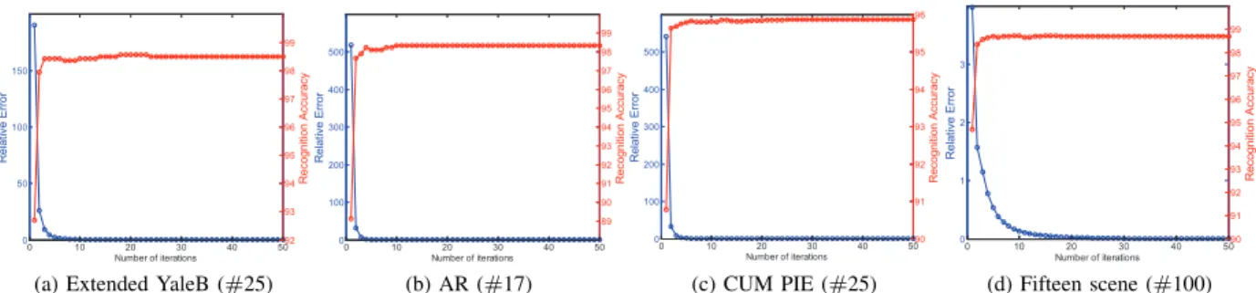
Proof. The proof of Theorem 5 is similar to Theorem 4. Although each exact minimum of the augmented La-grangian of the Algorithms 1 and 3 guarantees a sound convergence property, it is impractical to obtain an exact solution in each iteration. The inner loop of BCD embedded in the main loop of ALM is time consuming. It is very common to boost up the computation time of ALM via inexact solution of the subproblems. Precision in each iteration is favored but not indispensable. In many cases the convergence of a recessive method could be preserved within a mild loss of precision in subproblems. Hence in this paper we speed up the Algorithm 1 and 3 by quitting the inner loop of BCD after one iteration. As a result the convergence issue may be questioned, but we empirically show in Section V-E that the convergence of the resulting inexact ALM is well preserved.
V. EXPERIMENTALEVALUATION
In this section, we evaluate the performance of our proposed methods on publicly available databases, and compare them with currently popular linear regression methods for different classification tasks, i.e. face recognition, objection recognition and scene categories recognition. All the experiments are run
10 times with random data splits of training and test samples, and then the average classification results are reported on different datasets. We test our proposed methods on six public databases for three main tasks. Specifically, the performance of face recognition task is evaluated on four face databases: Extended YaleB [37], CMU PIE [38], AR [39], LFW [40]. Object recognition and scene recognition are performed on COIL-100 [41] and fifteen scene categories databases [42], respectively. It is worth pointing out that these databases are commonly used in multi-category image recognition and the existing methods have achieved decent results. Thus, challenging recognition results are convincing enough to verify the superiority of our methods, and a number of related state-of-the-art classification methods are enumerated as follows.
1) SRC [15]: It is to learn sparse representation based regression model with the l1-norm regularization. Both reconstruction error and sparse codes are employed for classification.
2) LLC [19]: It is to learn a locality constrained regres-sion model for large scale image classification. Locality-constrained codes are used for classification.
3) CRC[18]: It is to learn a linear regression model by using all the training samples with the l2-norm regularization. Both reconstruction error and collaborative representation codes are used for classification.
4) LRC[17]: It is to learn a linear regression model by using each class of training samples with the l2-norm regu-larization. Similar to CRC, the reconstruction error and learned representation codes are used for classification. 5) LRLR[23]: It is to learn a low-rank regression model by
introducing the low-rank (nuclear norm) regularization. The learned projection matrix is used for classification. 6) LRRR [23]: It is to learn a low-rank ridge regression
model by adding a Frobenius norm regularization on linear regression loss. Similar to LRLR, the learned projection matrix is used for classification.
7) SLRR [23]: It is to learn a sparse low-rank regression for feature section by imposing sparsity constraint on the low-rank regression loss. The low-rank projection matrix and selected features are used for classification.
8) RPCA [22], [27]: It is to learn clean images by de-composing a data matrix into low-rank term and sparse noise term, and then SRC on the clean data is used for classification.
9) LatLRR [26]: It is to learn salient features from the original dataset, and then linear regression model (2) is used to learn projection matrix. Subsequently, the linear transformation of the salient features obtained by using the learned projection matrix is employed for classifica-tion.
10) LRSI[27]: It is to learn a low-rank structured incoherence dictionary with shared features, and then the SRC method on the learned dictionary is used for classification. 11) CBDS [28]: It is to learn the data representation of
training samples, test samples and dictionary with class-wise block-diagonal structure by imposing the low-rank regularization, and then the learned representation is used
for classification.
12) DLSR [7]: It is to learn a discriminative LSR model by enlarging the distance between different classes in regression targets. The learned projection matrix are used for classification.
13) SVM [43]: It is to utilize support vector machine with Gaussian kernel on raw image features for classification. We use the LibSVM software [43]. Note that there exists an important regularization parameterCin SVM. A cross validation approach is utilized to select it from the range of[0.001,0.01,1.0,10.0,100.0]. Actually, SVM is also a popular derivation of LSR model.
14) DENLR: The proposed model is to learn a compact and discriminative regression model by imposing the elastic-net regularization and enlarging the margin of the regression targets. The objective function is Eqn. (13). To justify the effectiveness of theϵ-dragging technique, we remove theϵ-dragging term, i.e.E⊙M, from Eqn.(13), and denote it asENLR* in the experiments.
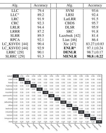
15) MENLR: The proposed model is to learn a marginal-ized regression model by embedding the marginalmarginal-ized constraint of the regression targets into the elastic-net regularized framework, which is presented in Eqn. (14). For fair comparison, we directly use the Matlab codes from the corresponding authors with the optimal parameter settings, or directly cite the experimental results from their original pa-pers. Specifically, to guarantee the same experimental settings between all the compared methods and our methods on each benchmark, we re-implemented all the methods using opti-mal parameters via tenfold cross validation, and the training and test samples were randomly selected from each dataset. Moreover, the experimental settings on scene recognition is the same as that of the LC-KSVD [42] method, and we directly cite some experimental results from the original paper. For the compared methods that are not included in [42], we rerun them following the same experimental settings in [42]. Therefore, all the methods presented in our paper are performed for each dataset on the same testbed such that our experimental results are convincing and reliable.
A. Face Recognition Evaluation
In this section, we evaluate the performances of our method for face recognition on four face databases.
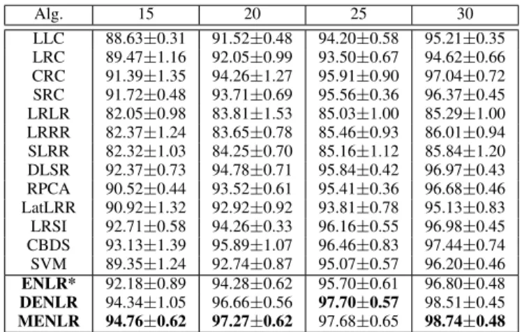
The Extended YaleB Database: The extended YaleB database contains 2414 front face images of 38 individuals and each subject has around 64 near frontal images under different illuminations. We randomly select 15, 20, 25, 30 images per subject for training, and the rest for testing. For all the compared methods, we exploit the suggested parameters in their papers for classification. The number of neighbors of LLC algorithm is set to fifteen, which is suggested as the best parameter for this dataset. Each image in this database for our experiments has been simply resized to 32×32 pixels. The classification accuracies of different methods on this database are summarized in Table I. Note that the mean classification accuracy and corresponding standard deviation (acc±std) are reported, and the bold numbers suggest the best classification
TABLE I: Classification accuracies (mean ± std %) of dif-ferent methods with difdif-ferent numbers of training samples on the Extended YaleB database. The bold numbers are the best classification accuracy. Alg. 15 20 25 30 LLC 88.63±0.31 91.52±0.48 94.20±0.58 95.21±0.35 LRC 89.47±1.16 92.05±0.99 93.50±0.67 94.62±0.66 CRC 91.39±1.35 94.26±1.27 95.91±0.90 97.04±0.72 SRC 91.72±0.48 93.71±0.69 95.56±0.36 96.37±0.45 LRLR 82.05±0.98 83.81±1.53 85.03±1.00 85.29±1.00 LRRR 82.37±1.24 83.65±0.78 85.46±0.93 86.01±0.94 SLRR 82.32±1.03 84.25±0.70 85.16±1.12 85.84±1.20 DLSR 92.37±0.73 94.78±0.71 95.84±0.42 96.97±0.43 RPCA 90.52±0.44 93.52±0.61 95.41±0.36 96.68±0.46 LatLRR 90.92±1.32 92.92±0.92 93.81±0.78 95.13±0.83 LRSI 92.71±0.58 94.26±0.33 96.16±0.55 96.98±0.45 CBDS 93.13±1.39 95.89±1.07 96.46±0.83 97.44±0.74 SVM 89.35±1.24 92.74±0.87 95.07±0.57 96.20±0.46 ENLR* 92.18±0.89 94.28±0.62 95.70±0.61 96.80±0.48 DENLR 94.34±1.05 96.66±0.56 97.70±0.57 98.51±0.45 MENLR 94.76±0.62 97.27±0.62 97.68±0.65 98.74±0.48
TABLE II: p-values between the proposed DENLR and MENLR methods and other methods on the Extended YaleB database.
Alg. 15 DENLR 25 15 MENLR 25
LLC 2.09×10⁻¹⁰ 2.95×10⁻¹² 3.48×10⁻¹² 1.50×10⁻¹¹ LRC 4.35×10⁻⁹ 2.05×10⁻¹³ 5.41×10⁻¹¹ 1.09×10⁻¹² CRC 3.55×10⁻⁵ 6.53×10⁻⁶ 1.46×10⁻⁶ 2.15×10⁻⁵ SRC 3.55×10⁻⁵ 2.09×10⁻¹² 3.83×10⁻¹⁰ 1.08×10⁻¹⁰ LRLR 4.95×10⁻¹⁶ 2.09×10⁻¹⁹ 6.61×10⁻¹⁸ 4.93×10⁻¹⁹ LRRR 4.55×10⁻¹⁷ 1.54×10⁻¹⁹ 8.67×10⁻²⁰ 4.33×10⁻¹⁹ SLRR 4.64×10⁻¹⁶ 1.09×10⁻¹⁷ 4.51×10⁻¹⁸ 2.03×10⁻¹⁷ DLSR 2.42×10⁻⁴ 1.33×10⁻⁹ 6.22×10⁻⁷ 2.78×10⁻⁸ RPCA 6.56×10⁻¹² 2.50×10⁻⁷ 2.09×10⁻¹⁰ 7.64×10⁻⁷ LatLRR 4.76×10⁻⁶ 1.75×10⁻¹¹ 1.33×10⁻⁷ 6.01×10⁻¹¹ LRSI 4.47×10⁻⁴ 2.51×10⁻⁷ 1.60×10⁻⁶ 1.86×10⁻⁶ CBDS 0.0412 6.87×10⁻⁴ 3.3×10⁻³ 2.3×10⁻³ SVM 1.38×10⁻⁸ 5.02×10⁻¹¹ 3.16×10⁻¹⁰ 4.39×10⁻¹⁰
accuracies. From Table I, it is clear to see that our method can consistently achieve the best classification accuracies with varying number of training samples. Moreover, we can see that if we remove the relax term of the regression target matrix, the performance of ENLR* is obviously better than other LSR methods, such as LRC, SRC, LRLR, LRRR and SLRR. This also reflects the fact that the elastic-net regularization term can lead to a more compact projection matrix such that higher classification accuracies can be achieved. Moreover, DENLR and MENLR can achieve the best classification accuracies in comparison with all the compared algorithms.
In addition, we conducted a statistical significance test for the results summarized in Table I to judge the significant improvements of the developed models in comparison with the state-of-the-art regression methods. The significance level, i.e. p-value, is typically set to 0.05, which means that if the significance evaluation is lower than this level, the perfor-mance difference between the evaluated methods is statistically significant. The p-values between the proposed DENLR and MENLR methods and the compared methods are shown in Table II, when the number of training samples for each subject
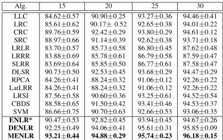
TABLE III: Classification accuracies (mean±std %) of differ-ent methods with differdiffer-ent numbers of training samples on the CMU PIE database.
Alg. 15 20 25 30 LLC 84.62±0.57 90.90±0.25 93.27±0.36 94.46±0.41 LRC 85.61±0.62 90.17±0.52 92.65±0.38 94.01±0.22 CRC 89.76±0.59 92.42±0.29 93.80±0.29 94.61±0.12 SRC 88.97±0.66 91.14±0.39 92.62±0.38 93.71±0.18 LRLR 83.70±0.57 85.73±0.58 86.80±0.45 87.62±0.48 LRRR 83.88±0.69 85.78±0.61 86.79±0.58 87.59±0.47 SLRR 83.69±0.64 85.85±0.50 86.77±0.61 87.58±0.47 DLSR 90.73±0.50 92.53±0.45 93.68±0.29 94.47±0.29 RPCA 84.26±0.41 88.24±0.32 91.06±0.12 92.26±0.22 LatLRR 84.26±0.41 88.24±0.32 91.06±0.12 92.26±0.22 LRSI 87.56±0.58 90.60±0.36 93.25±0.61 94.52±0.54 CBDS 88.58±0.65 91.50±0.42 93.41±0.46 94.53±0.37 SVM 86.66±0.75 90.70±0.63 92.66±0.53 93.06±0.35 ENLR* 90.47±0.53 92.82±0.45 93.94±0.45 94.67±0.26 DENLR 92.25±0.49 94.06±0.41 95.61±0.31 95.85±0.09 MENLR 93.21±0.44 94.88±0.29 95.74±0.23 96.18±0.15
is set to15and25. We can see that the performance differences between our methods and all the compared methods are statistically significant, which also improves the effectiveness of our methods.
The CMU PIE Database: The CMU PIE face database contains 41,368 face images from 68 subjects as a whole. The images under five near frontal poses (C05, C07, C09, C27 and C29) are used in our experiment. We randomly select 15, 20, 25, 30 images from each subject as training samples and the remaining images as test samples. The classification rates using different methods are summarized in Table III. We can see that our methods DENLR and MENLR always outperform the compared methods in different cases, and the performance of ENLR* in most cases is better than or competitive with all the compared methods.
The AR Database: The AR face database contains about 4,000 color face images of 126 subject, which consist of the frontal faces with different facial expressions, illuminations and disguises. In this experiment, we select a subset including 2600 images from 50 female and 50 male subjects. We randomly select 8, 11, 14, 17 images for each subject as training samples and the rest of images as test samples. Following the implementation in [44], each image is project-ed onto a 540-dimensional feature vector with a randomly generated matrix from a zero-mean normal distribution. The experimental results obtained by using different classification methods are shown in Table IV. Apparently, our methods in most cases achieve the best classification results, which also verify that the proposed regression models outperform all the other regression models under different training conditions.
The LFW Database:The Labeled Faces in the Wild (LFW) face database is designed for the study of unconstrained identity verification and face recognition. It contains more than 13,000 face images from 1680 subject pictured under the unconstrained conditions. In this experiment, we use a subset including 1251 images from 86 peoples and each subject has only 10-20 images [45]. Each image was manually cropped and resized to 32 × 32 pixels. We randomly choose 5, 6, 7, 8 images of each subject as training samples, and the
TABLE IV: Classification accuracies (mean±std %) of differ-ent methods with differdiffer-ent numbers of training samples on the AR database. Alg. 8 11 14 17 LLC 54.26±1.27 60.87±0.91 66.88±1.03 71.58±1.32 LRC 63.87±1.42 76.87±1.13 85.20±1.00 90.88±0.97 CRC 86.53±1.07 91.66±0.77 94.06±0.77 95.74±0.76 SRC 84.08±0.98 89.45±0.74 92.20±1.19 95.14±0.67 LRLR 76.75±1.37 88.93±0.86 93.02±0.63 94.92±0.68 LRRR 91.40±0.71 93.82±0.70 95.42±0.48 96.47±0.70 SLRR 90.02±0.76 93.70±0.55 95.15±0.70 96.04±0.49 DLSR 89.56±0.68 93.65±0.67 94.36±0.62 95.18±0.46 RPCA 77.32±1.43 84.39±1.33 88.82±0.90 92.62±0.77 LatLRR 88.42±0.76 92.13±1.06 95.96±0.70 97.13±0.80 LRSI 78.78±1.02 85.93±1.01 89.92±0.76 93.17±0.97 CBDS 88.65±0.73 92.92±0.69 95.17±0.60 96.63±0.63 SVM 75.74±1.60 86.19±1.02 91.99±0.70 95.08±0.91 ENLR* 90.42±0.87 93.80±0.83 95.41±0.68 96.31±0.56 DENLR 91.94±0.80 95.69±0.70 97.30±0.62 98.21±0.54 MENLR 92.61±0.64 95.63±0.75 97.16±0.59 98.56±0.61
TABLE V: Classification accuracies (mean±std %) of differ-ent methods with differdiffer-ent numbers of training samples on the LFW database. Alg. 5 6 7 8 LLC 27.42±1.42 29.50±1.59 31.06±1.25 31.90±0.80 LRC 29.88±1.58 33.13±1.76 35.42±1.79 37.23±1.86 CRC 29.54±1.16 31.72±1.22 32.86±1.36 33.81±1.32 SRC 29.03±1.57 32.21±1.53 33.36±2.00 36.21±2.54 LRLR 29.88±1.02 30.18±0.74 34.45±1.63 35.16±2.17 LRRR 30.58±1.39 32.83±1.74 34.80±1.33 36.48±1.77 SLRR 30.72±1.23 33.02±1.53 35.32±1.41 36.40±1.69 DLSR 31.22±0.83 33.81±1.53 35.87±1.60 37.02±1.58 RPCA 29.82±1.59 32.52±1.36 34.45±1.63 36.27±1.43 LatLRR 29.96±1.06 33.22±1.85 35.30±1.90 37.12±1.65 LRSI 29.51±1.91 32.16±1.34 34.62±1.49 36.61±1.65 CBDS 31.13±1.44 32.83±1.46 34.30±1.52 36.30±1.82 SVM 29.66±1.64 32.36±1.70 35.46±1.42 36.73±1.45 ENLR* 30.66±1.01 33.28±2.13 35.22±1.67 36.41±1.87 DENLR 32.69±1.26 36.04±1.43 38.32±1.51 40.09±1.80 MENLR 34.97±1.35 37.13±1.37 39.79±1.29 41.26±1.65
remaining face images are exploited as test samples. Because the LFW database is a very difficult database for image classification, the accuracies obtained by utilizing different classification methods are comparatively not high, but the highest classification accuracies are still established by using our methods, which again certify the effectiveness of the proposed methods.
Overall, the proposed ENLR methods outperform all the compared regression methods on the four face image databas-es, which demonstrates that our methods can effectively solve the face recognition problem.
B. Object Recognition Evaluation
To verify the assumption that our methods are feasible to solve object recognition task, we evaluate the performances of our methods on Columbia Object Image Library (COIL-100) database [41], which contains various views of 100 objects with different lighting conditions. In our experiments, the images are converted to gray-scale images with the 32 × 32 pixels, and then the robustness is evaluated on alternative viewpoints. We randomly select 15, 20, 25, 30 images per