Portland State University
PDXScholar
Dissertations and Theses Dissertations and Theses
12-1-2016
Using Blind Source Separation and a Compact Microphone Array
to Improve the Error Rate of Speech Recognition
Jeffrey Dean Hoffman
Portland State University
Let us know how access to this document benefits you.
Follow this and additional works at:http://pdxscholar.library.pdx.edu/open_access_etds Part of theElectrical and Computer Engineering Commons
Recommended Citation
Hoffman, Jeffrey Dean, "Using Blind Source Separation and a Compact Microphone Array to Improve the Error Rate of Speech Recognition" (2016).Dissertations and Theses.Paper 3367.
Using Blind Source Separation andaCompact Microphone Arrayto Improve the Error RateofSpeech Recognition
by
Jeffrey Dean Hoffman
A thesis submitted in partial fulfillment of the requirements for the degree of
Master of Science in
Electrical and Computer Engineering
Thesis Committee: James McNames, Chair
Y. C. Jenq Fu Li
Portland State University 2016
Abstract
Automatic speech recognition has become a standard feature on many consumer electronics and automotive products, and the accuracy of the decoded speech has improved dramatically over time. Often, designers of these products achieve accuracy by employing microphone arrays and beamforming algorithms to reduce interference. However, beamforming microphone arrays are too large for small form factor products such as smart watches. Yet these small form factor products, which have precious little space for tactile user input (i.e. knobs, buttons and touch screens), would benefit immensely from a user interface based on reliably accurate automatic speech recognition.
This thesis proposes a solution for interference mitigation that employs blind source separation with a compact array of commercially available unidirectional microphone elements. Such an array provides adequate spatial diversity to enable blind source separation and would easily fit in a smart watch or similar small form factor product. The solution is characterized using publicly available speech audio clips recorded for the purpose of testing automatic speech recognition algorithms. The proposal is modelled in different interference environments and the efficacy of the solution is evaluated. Factors affecting the performance of the solution are identified and their influence quantified. An expectation is presented for the quality of separation as well as the resulting improvement in word error rate that can be achieved from decoding the separated speech estimate versus the mixture obtained from a single unidirectional microphone element. Finally, directions for future work are proposed, which have the potential to improve the performance of the solution thereby making it a commercially viable product.
Acknowledgments
First, I want to thank each of my instructors at Portland State University for imparting to me their knowledge. It is only by standing on their shoulders that I am equipped to support this thesis. Second, I want to thank my thesis committee, particularly my advisor Dr. James McNames. His careful review, thoughtful guidance, and high standards propelled me toward a destination far beyond my own myopic limitations. Third, I want to thank my coworkers for their steadfast support and encouragement. The process was more bearable having people in my corner cheering me on. Most of all, I want thank my wife Meg for the many sacrifices and accommodations that she made as I pursued my dream. If I have achieved anything at all useful here, a large share of the credit I owe to her.
Table of Contents Abstract ... i Acknowledgments... ii List of Tables ... iv List of Figures ... vi Chapter 1. Introduction ... 1
Chapter 2. Literature Review... 8
Chapter 3. Methods... 42
Chapter 4. Results and Discussion ... 53
Chapter 5. Conclusions ... 131
List of Tables
Table 1. Overall improvement in SIR with the small room model. ... 56
Table 2. ANOVA on SIR improvement by speaker using the natural gradient IVA algorithm and SSL prior with the small room model. ... 64
Table 3. ANOVA on SIR improvement by speaker using the natural gradient IVA algorithm and Liang’s prior with the small room model. ... 69
Table 4. ANOVA on SIR improvement by speaker using the fixed-point IVA algorithm and SSL prior with the small room model. ... 74
Table 5. ANOVA on SIR improvement by speaker using the fixed-point IVA algorithm and Liang’s prior with the small room model. ... 78
Table 6. ANOVA on SIR improvement by speaker using the real time IVA algorithm and SSL prior with the small room model. ... 83
Table 7. ANOVA on SIR improvement by speaker using the real time IVA algorithm and Liang’s prior with the small room model. ... 88
Table 8. ANOVA on SIR improvement by speaker using the auxiliary function IVA algorithm and SSL prior with the small room model. ... 93
Table 9. ANOVA on SIR improvement by speaker using the auxiliary function IVA algorithm and Liang’s prior with the small room model. ... 98
Table 10. Overall improvement in SDR with the small room model. ... 99
Table 11. Overall change in SAR with the small room model. ... 102
Table 12. Overall improvement in WER by algorithm using the small room model. .... 106
Table 13. Overall improvement in SIR with the large room model. ... 110
Table 14. Overall improvement in SDR with the large room model. ... 112
Table 15. Overall change in SAR with the large room model. ... 114
Table 16. Overall improvement in WER by algorithm using the large room model. ... 118
Table 17. Overall improvement in SIR with the corner room model. ... 121
List of Figures
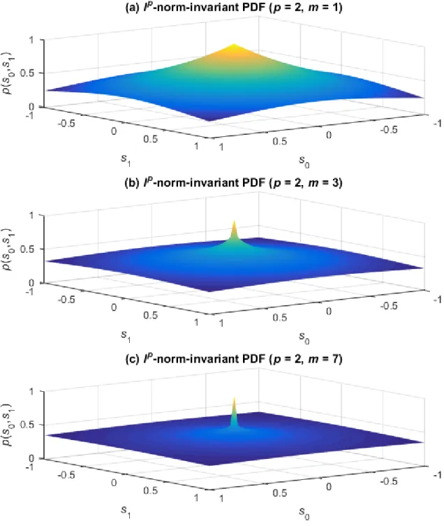
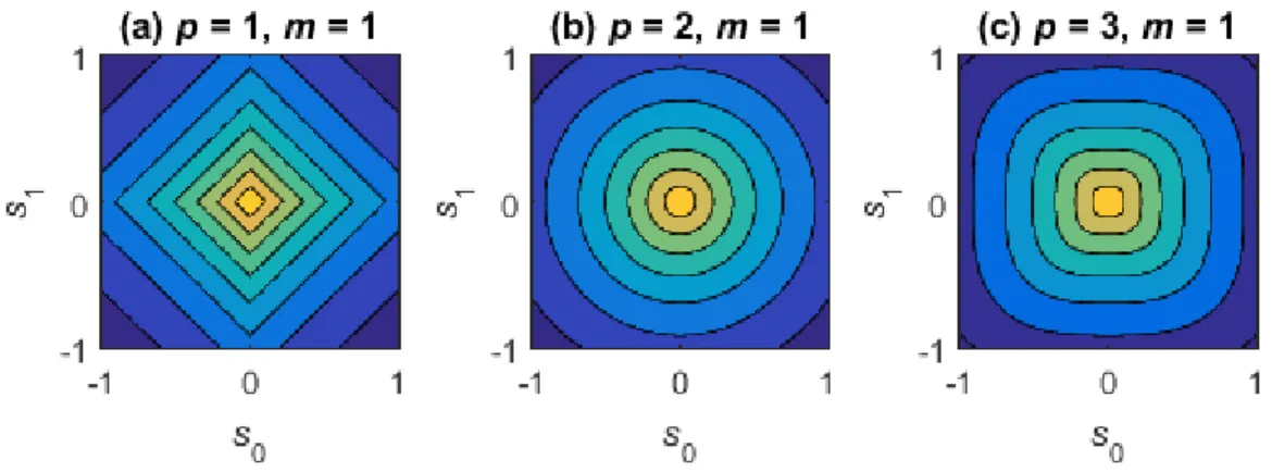
Figure 1. Diagram of the physical mixing and blind source separation processes with two speakers and two microphones. ... 3 Figure 2. Amplitude histogram of the clean speech phrase “although trees that chance to stand alone outside the groves sweep forth long curved branches producing a striking contrast to the ordinary grove form.” ... 9 Figure 3. Diagram of the frequency domain separation process for convolved mixtures. 21 Figure 4. Spectrogram of American-English phrase “although trees that chance to stand alone outside the groves sweep forth long curved branches producing a striking contrast to the ordinary grove form.” ... 22 Figure 5. Plots of (a) discrete time sampled 4.0, 4.5 and 5.0 Hz sinusoids and (b) their magnitude spectrum at 1.0 Hz resolution. ... 25 Figure 6. Plots (a) and (c) are discrete time samples of 1 second rectangular and Hann windows. Plots (b) and (d) are their magnitude spectrums at 0.5 Hz resolution. ... 26 Figure 7. Plots of independent and spherically symmetric bivariate Laplacian distributions. The white curves show conditional probability 𝑝𝑠0𝑠1 = 1. ... 30 Figure 8. The effect of sparsity parameter 𝑚 on the 𝑙𝑝-norm-invariant multivariate probability density function. Plot (a) shows the SSL prior. Plot (b) shows Liang’s prior with increased sparsity (a narrower peak). Plot (c) shows I. Lee’s prior with even greater sparsity than Liang’s. ... 39 Figure 9. The effect of symmetry control parameter 𝑝 on the 𝑙𝑝-norm-invariant multivariate probability density function. Contour plot (a) shows linear symmetry. Contour plot (b) shows spherical symmetry. Contour plot (c) show cubic symmetry. ... 40 Figure 10. A slice of an image space showing a portion of an x-y plane containing microphone M and speaker S. The physical room lies adjacent to the origin and is bounded by thick lines. Images of the room unfold outward toward infinity in 3D space. Trajectory p1 has a single reflection and p2 has two reflections. Virtual trajectories of trajectories p1 and p2 are shown as dashed lines. ... 43 Figure 11. The gain of the PUM-3046L-R depends on the angle ψ between the longitudinal axis x and the vector to the source s. Gain is circularly symmetric around the longitudinal axis. The microphone is shown oriented with its longitudinal axis coincident with the x -axis and its face in the y-z plane pointing in the positive x direction... 45
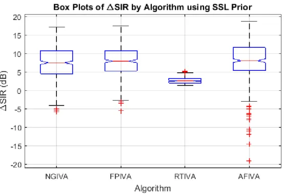
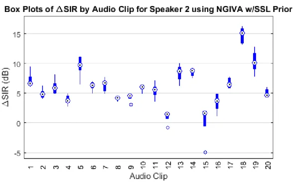
Figure 12. Relative gain vs. azimuth curves in the x-y plane for a four-element microphone array constructed from PUM-3046L-R directional microphones oriented at 90° angles in the x-y plane. ... 47 Figure 13. Relative gain surface of a four element microphone array constructed from PUM-3046L-R directional microphones oriented at 90° angles in the x-y plane. Relative gain along a speech source vector passing through a point on the surface and terminating at the origin where the microphones are located is indicated by both the color at that point and the length of the line segment between the point and the origin. ... 48 Figure 14. Diagram of a small 3 m by 4 m room layout showing the locations of the microphone array (gray diamond), speaker of interest (red square), and interfering speakers (blue circles). The geometry models the use case of a microphone array equipped smart watch. ... 55 Figure 15. Box plots of SIR improvement by algorithm using the SSL prior with the small room model. ... 57 Figure 16. Box plots of SIR improvement by algorithm using the Liang’s prior with the small room model. ... 57 Figure 17. Box plots of SIR improvement by speaker using the natural gradient IVA algorithm and SSL prior with the small room model. ... 59 Figure 18. Box plots of SIR improvement for speaker 1 by audio clip using natural gradient IVA and SSL prior with the small room model. ... 60 Figure 19. Box plots of SIR improvement for speaker 2 by audio clip using natural gradient IVA and SSL prior with the small room model. ... 60 Figure 20. Box plots of SIR improvement for speaker 3 by audio clip using natural gradient IVA and SSL prior with the small room model. ... 61 Figure 21. Box plots of SIR improvement for speaker 4 by audio clip using natural gradient IVA and SSL prior with the small room model. ... 61 Figure 22. Normal probability plot of SIR improvement by speaker using the natural gradient IVA algorithm and SSL prior with the small room model. ... 62 Figure 23. Box plots of SIR improvement by speaker using the natural gradient IVA algorithm and Liang’s prior with the small room model. ... 65 Figure 24. Box plots of SIR improvement for speaker 1 by audio clip using natural gradient IVA and Liang’s prior with the small room model... 66 Figure 25. Box plots of SIR improvement for speaker 2 by audio clip using natural gradient IVA and Liang’s prior with the small room model... 66
Figure 26. Box plots of SIR improvement for speaker 3 by audio clip using natural gradient IVA and Liang’s prior with the small room model... 67 Figure 27. Box plots of SIR improvement for speaker 4 by audio clip using natural gradient IVA and Liang’s prior with the small room model... 67 Figure 28. Normal probability plot of SIR improvement by speaker using the natural gradient IVA algorithm and Liang’s prior with the small room model. ... 68 Figure 29. Box plots of SIR improvement by speaker using the fixed-point IVA algorithm and SSL prior with the small room model. ... 70 Figure 30. Box plots of SIR improvement for speaker 1 by audio clip using fixed-point IVA and SSL prior with the small room model. ... 71 Figure 31. Box plots of SIR improvement for speaker 2 by audio clip using fixed-point IVA and SSL prior with the small room model. ... 71 Figure 32. Box plots of SIR improvement for speaker 3 by audio clip using natural gradient IVA and SSL prior with the small room model. ... 72 Figure 33. Box plots of SIR improvement for speaker 4 by audio clip using fixed-point IVA and SSL prior with the small room model. ... 72 Figure 34. Normal probability plot of SIR improvement by speaker using the fixed-point IVA algorithm and SSL prior with the small room model. ... 73 Figure 35. Box plots of SIR improvement by speaker using the fixed-point IVA algorithm and Liang’s prior with the small room model. ... 74 Figure 36. Box plots of SIR improvement for speaker 1 by audio clip using fixed-point IVA and Liang’s prior with the small room model... 75 Figure 37. Box plots of SIR improvement for speaker 2 by audio clip using fixed-point IVA and Liang’s prior with the small room model... 76 Figure 38. Box plots of SIR improvement for speaker 3 by audio clip using natural gradient IVA and Liang’s prior with the small room model... 76 Figure 39. Box plots of SIR improvement for speaker 4 by audio clip using fixed-point IVA and Liang’s prior with the small room model... 77 Figure 40. Normal probability plot of SIR improvement by speaker using the fixed-point IVA algorithm and Liang’s prior with the small room model. ... 78 Figure 41. Box plots of SIR improvement by speaker using the real time IVA algorithm
Figure 42. Box plots of SIR improvement for speaker 1 by audio clip using real time IVA and SSL prior with the small room model. ... 80 Figure 43. Box plots of SIR improvement for speaker 2 by audio clip using real time IVA and SSL prior with the small room model. ... 81 Figure 44. Box plots of SIR improvement for speaker 3 by audio clip using natural gradient IVA and SSL prior with the small room model. ... 81 Figure 45. Box plots of SIR improvement for speaker 4 by audio clip using real time IVA and SSL prior with the small room model. ... 82 Figure 46. Normal probability plot of SIR improvement by speaker using the real time IVA algorithm and SSL prior with the small room model. ... 83 Figure 47. Box plots of SIR improvement by speaker using the real time IVA algorithm and Liang’s prior with the small room model. ... 84 Figure 48. Box plots of SIR improvement for speaker 1 by audio clip using real time IVA and Liang’s prior with the small room model. ... 85 Figure 49. Box plots of SIR improvement for speaker 2 by audio clip using real time IVA and Liang’s prior with the small room model. ... 86 Figure 50. Box plots of SIR improvement for speaker 3 by audio clip using natural gradient IVA and Liang’s prior with the small room model... 86 Figure 51. Box plots of SIR improvement for speaker 4 by audio clip using real time IVA and Liang’s prior with the small room model. ... 87 Figure 52. Normal probability plot of SIR improvement by speaker using the real time IVA algorithm and Liang’s prior with the small room model. ... 88 Figure 53. Box plots of SIR improvement by speaker using the auxiliary function IVA algorithm and SSL prior with the small room model. ... 89 Figure 54. Box plots of SIR improvement for speaker 1 by audio clip using auxiliary function IVA and SSL prior with the small room model... 90 Figure 55. Box plots of SIR improvement for speaker 2 by audio clip using auxiliary function IVA and SSL prior with the small room model... 91 Figure 56. Box plots of SIR improvement for speaker 3 by audio clip using natural gradient IVA and SSL prior with the small room model. ... 91 Figure 57. Box plots of SIR improvement for speaker 4 by audio clip using auxiliary function IVA and SSL prior with the small room model... 92
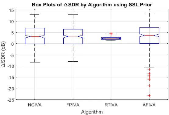
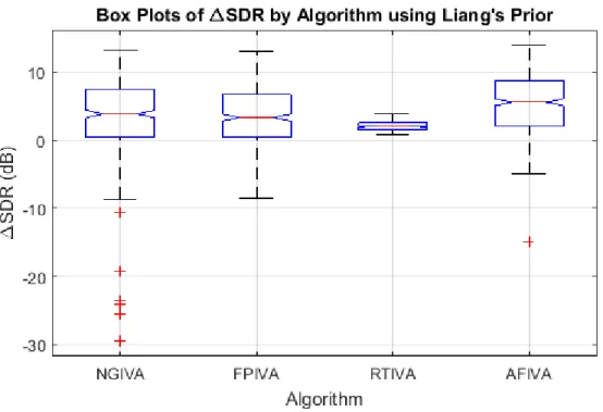
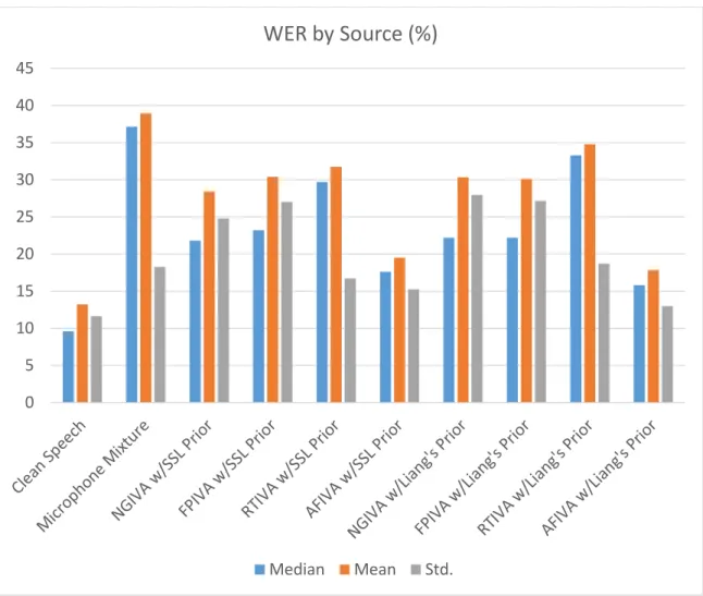
Figure 58. Normal probability plot of SIR improvement by speaker using the auxiliary function IVA algorithm and SSL prior with the small room model. ... 93 Figure 59. Box plots of SIR improvement by speaker using the auxiliary function IVA algorithm and Liang’s prior with the small room model. ... 94 Figure 60. Box plots of SIR improvement for speaker 1 by audio clip using auxiliary function IVA and Liang’s prior with the small room model. ... 95 Figure 61. Box plots of SIR improvement for speaker 2 by audio clip using auxiliary function IVA and Liang’s prior with the small room model. ... 96 Figure 62. Box plots of SIR improvement for speaker 3 by audio clip using auxiliary function IVA and Liang’s prior with the small room model. ... 96 Figure 63. Box plots of SIR improvement for speaker 4 by audio clip using auxiliary function IVA and Liang’s prior with the small room model. ... 97 Figure 64. Normal probability plot of SIR improvement by speaker using the auxiliary function IVA algorithm and Liang’s prior with the small room model. ... 98 Figure 65. Box plots of SDR improvement by algorithm using the SSL prior with the small room model. ... 100 Figure 66. Box plots of SDR improvement by algorithm using the Liang’s prior with the small room model. ... 101 Figure 67. Box plots of the change in SAR by algorithm using the SSL prior with the small room model. ... 103 Figure 68. Box plots of the change in SAR by algorithm using the Liang’s prior with the small room model. ... 104 Figure 69. WER of decoded clean speech, microphone mixture, and separated source estimates using the small room model. ... 105 Figure 70. Box plots of WER improvement by algorithm using the SSL prior with the small room model. ... 107 Figure 71. Box plots of WER improvement by algorithm using Liang’s prior with the small room model. ... 108 Figure 72. Diagram of a large 5 m by 4 m room layout showing the locations of the microphone array (gray diamond), speaker of interest (red square), and interfering speakers (blue circles). The geometry models the use case of a microphone array equipped smart
Figure 73. Box plots of SIR improvement by algorithm using the SSL prior with the large room model. ... 111 Figure 74. Box plots of SIR improvement by algorithm using the Liang’s prior with the large room model. ... 111 Figure 75. Box plots of SDR improvement by algorithm using the SSL prior with the large room model. ... 113 Figure 76. Box plots of SDR improvement by algorithm using the Liang’s prior with the large room model. ... 113 Figure 77. Box plots of SAR improvement by algorithm using the SSL prior with the large room model. ... 115 Figure 78. Box plots of SAR improvement by algorithm using the Liang’s prior with the large room model. ... 115 Figure 79. WER of decoded clean speech, microphone mixture, and separated source estimates using the large room model. ... 117 Figure 80. Box plots of WER improvement by algorithm using the SSL prior with the large room model. ... 119 Figure 81. Box plots of WER improvement by algorithm using Liang’s prior with the large room model. ... 119 Figure 82. Diagram of a large 5 m by 4 m room layout showing the locations of the microphone array (gray diamond), speaker of interest (red square), and interfering speakers (blue circles). The geometry models the use case of a microphone array equipped smart watch located at one corner of the room. ... 120 Figure 83. Box plots of SIR improvement by algorithm using the SSL prior with the corner room model. ... 122 Figure 84. Box plots of SIR improvement by algorithm using the Liang’s prior with the corner room model. ... 122 Figure 85. Box plots of SDR improvement by algorithm using the SSL prior with the corner room model. ... 124 Figure 86. Box plots of SDR improvement by algorithm using the Liang’s prior with the corner room model. ... 124 Figure 87. Box plots of SAR improvement by algorithm using the SSL prior with the corner room model. ... 126
Figure 88. Box plots of SAR improvement by algorithm using the Liang’s prior with the corner room model. ... 126 Figure 89. WER of decoded clean speech, microphone mixture, and separated source estimates using the corner room model. ... 128 Figure 90. Box plots of WER improvement by algorithm using the SSL prior with the corner room model. ... 130 Figure 91. Box plots of WER improvement by algorithm using Liang’s prior with the corner room model. ... 130 Figure 92. Spectrograms of clean speech, the mixture at the microphone element pointed at the speaker of interest, and the separated source estimated produced by AFIVA. ... 133
Chapter 1. Introduction
Automatic speech recognition (ASR) has become a standard feature on many consumer electronics products such as personal computers, laptops, tablets, smartphones and automotive infotainment systems. ASR technology is mature and deemed reliable enough even for use in military applications such as the F-16 and F-35 fighter aircraft [1], [2]. However, ASR systems have difficulty dealing with acoustic interference [3]. This phenomenon is known as the “cocktail party problem.” Speech that is perfectly understood in a quiet environment is rendered unintelligible in an environment with many interfering sources such as a cocktail party. This problem diminishes accuracy of speech recognition in humans and ASR equipped devices alike.
1.1 Background
Microphone arrays have been used extensively to mitigate impairment due to interference and noise. These are used along with signal processing algorithms that fall primarily into one of two categories: beamforming or blind source separation (BSS). Great results have been obtained using beamforming when target and interferer locations are known [4], [5]. A number of researchers have combined beamforming with BSS and obtained great results even when locations are unknown [6]-[8]. However, beamforming has a limitation that is problematic for small form factor devices such as smart watches and fitness bands. The speed of sound through air is roughly 340 m/s, and the bandwidth of speech is roughly 3400 Hz. For ½ wavelength phase shift at the upper end of the speech spectrum, the microphone array must have an aperture of at least 5 cm. For beamforming at the lower
end of the speech spectrum, a much larger aperture is required. Small form factor devices such as smart watches and fitness bands cannot support a microphone array of this size.
Yet, small form factor devices could benefit immensely from ASR. Surface area for traditional tactile user interfaces (i.e. touch screen display, buttons and knobs) is extremely limited on these devices. With the current state of the art in ASR, the user could issue nearly unlimited commands or dictate text and email messages of arbitrary content hands free. However, it is unlikely that the user will be content with ASR that only functions robustly in a quiet environment. Since the physical dimensions of these devices do not support the microphone array requirements of beamforming, a BSS alternative is an attractive option for improving the reliability of ASR.
While BSS implementations often result in beamforming, beamforming is not necessarily required. Spatial diversity is a sufficient condition for separation of statistically independent sources. Spatial diversity in this context means that the speech signals reaching different microphones from the same source arrive with different amplitudes in the case of instantaneous mixing or different spectrums in the case of convolutive mixing. A diagram of the physical mixing and blind source separation processes for a two-speaker two-microphone system is shown in Figure 1.
Figure 1. Diagram of the physical mixing and blind source separation processes with two speakers and two microphones.
In the simplest (although not very realistic) case, speakers 𝑠𝑗 are instantaneously
mixed through unequal gains 𝑎𝑖𝑗 into microphones 𝑥𝑖. Using linear algebra, we write this
as1 𝐱 = 𝐀𝐬 (1) which is equivalent to 𝑥𝑖 = ∑ 𝑎𝑖𝑗𝑠𝑗 𝑛 𝑗=1 , 𝑖 = {1, … , 𝑚}, 𝑛 ≤ 𝑚 (2)
where 𝐱 is an 𝑚 × 1 vector, 𝐀 is an 𝑚 × 𝑛 matrix, 𝐬 is an 𝑛 × 1 vector and in this simple case 𝑚 = 𝑛 = 2.
The goal of blind source separation in this simplest of cases is to estimate gains 𝑤𝑖𝑗
that form the demixing matrix 𝐖, which is the inverse of the mixing matrix 𝐀. Demixing
1 In mathematical equations throughout this document, vectors and functions returning vectors are non-italicized bold lowercase, matrices and functions returning matrices are non-non-italicized bold uppercase, scalars and functions returning scalars are italicized non-bold, with the exception that well-known predefined functions returning scalars such as log(·) and exp(·) are non-italicized non-bold lower case.
a
11x
1s
1a
22x
2s
2u
1w
11w
22u
2Blind Source Separation
Physical Mixing Process
matrix 𝐖 can then be used along with microphones 𝑥𝑖 to produce estimates 𝑢𝑗 of speakers
𝑠𝑗 that are optimal in some sense (e.g., least squares) without knowing the value of the mixing matrix 𝐀. Using linear algebra, we write the final step as
𝐮 = 𝐖𝐱 = 𝐀̂−1𝐱 = 𝐬̂ (3) which is equivalent to 𝑢𝑗 = ∑ 𝑤𝑗𝑖𝑥𝑖 𝑚 𝑖=1 , 𝑗 = {1, … , 𝑛}, 𝑛 ≤ 𝑚 (4)
where 𝐮 is an 𝑛 × 1 vector and 𝐖 is the 𝑛 × 𝑚 matrix that is an estimate of the inverse of
𝐀. For a rectangular matrix 𝐀 of rank 𝑚, we define its inverse 𝐀−1 as the matrix satisfying
𝐀−1𝐀 = 𝐈 (5)
and the estimate of its inverse
𝐖 = 𝐀̂−1 (6)
In our simple case, the 2 × 2 matrix 𝐀 is invertible if and only if it is non-singular (i.e. its determinant must not equal zero). The determinant of 𝐀 is
det(𝐀) = |𝑎𝑎11 𝑎12
21 𝑎22| = 𝑎11𝑎22− 𝑎21𝑎12 (7)
Referring back to Figure 1 and equation (7), we see that if the gains 𝑎11 and 𝑎21 from
speaker 𝑠1 to microphones 𝑥1 and 𝑥2 are equal and the gains 𝑎12 and 𝑎22 from speaker 𝑠2
to microphones 𝑥1 and 𝑥2 are also equal, then the determinant of 𝐀 is zero and 𝐀 is not invertible. Thus spatial diversity is a necessary condition for separation. In practice, problems can occur even if the matrix is invertible, but conditioned. With an ill-conditioned matrix, very small changes in 𝐱produce large changes in𝐮.
Finally, in the linear system of equation (1), we can only solve for the unknown quantities 𝑠𝑗 if the number of known quantities 𝑥𝑖 are equal to or greater than the number
of 𝑠𝑗. This is a fundamental property of systems of linear equations. Hence, the limitation
𝑛 ≤ 𝑚.
In a more realistic case, there are multiple paths for audio pressure waves to reach a particular microphone. This is referred to as a reverberant environment. As the pressure waves from an audio source bounce off solid objects like a floor, ceiling or walls, they arrive at a microphone at different times and strengths depending on the absorption of the various objects and the trajectory. This can be modelled in discrete time by replacing the coefficients of mixing matrix 𝐀 with IIR filters. Mixing is now a convolutive process where multiplication in the instantaneous case is replaced by convolution in the reverberant case. We write this mathematically as
𝑥𝑖[𝑡] = ∑ ∑ 𝑎𝑖𝑗[𝜏]𝑠𝑗[𝑡 − 𝜏] ∞ 𝜏=0 𝑛 𝑗=1 , 𝑖 = {1, … , 𝑚}, 𝑛 ≤ 𝑚 (8)
In practice, it is not necessary to implement an infinite length filter because the strength of the arriving pressure wave(s) diminishes rapidly as the trajectory increases in length. In order to reduce complexity, IIR filters may be replaced by FIR filters without significant loss of fidelity. Methods for predicting reverberation time based on the physical characteristics of the environment were published by Lehmann and Johansson [9] and are frequently cited in the literature.
Separation requires the estimation of the demixing matrix 𝐖 consisting of the inverse of the matrix of filters in 𝐀. Once estimated, demixing matrix 𝐖 is convolved with
microphone outputs 𝑥𝑖 to produce discrete time estimates 𝑢𝑗 of sources 𝑠𝑗. We write this mathematically as 𝑢𝑗 = ∑ ∑ 𝑤𝑗𝑖[𝜏]𝑥𝑖[𝑡 − 𝜏] ∞ 𝜏=0 𝑚 𝑖=1 , 𝑗 = {1, … , 𝑛}, 𝑛 ≤ 𝑚 (9)
While this problem is much more complex than the instantaneous case with many more parameters to be estimated, we shall see in Chapter 2 that the same fundamental techniques can be applied.
In my search of the literature on BSS for speech signals, all of the solutions relied on arrays of omnidirectional directional microphones with sufficient spacing for spatial diversity. An array of closely spaced omnidirectional microphones that would fit in a smart watch or fitness band would result in strongly correlated signals emanating from all microphone elements in the array. The mixing matrix would be nearly singular and therefore ill-conditioned.
Fortunately, unidirectional microphones as small as 6.0 × 3.2 mm and costing as little as $1.17 in quantity are commercially available today. Smaller models down to 2.56 × 2.74 mm and costing less than $20 are also commercially available. These microphones can be collocated in a way that provides spatial diversity by aiming them in different directions. Increased demand due to the improved user experience that robust ASR would bring to smart watches and fitness bands would result in economies of scale. Because the trend in electronic components is almost universally toward smaller and cheaper with economies of scale, it is reasonable to expect reductions in cost of the smaller unidirectional
1.2 Contribution of This Work
The small form factors achievable with directional microphone arrays make them suitable for integration into wearables like smart watches and fitness bands. Wearables that would benefit immensely from ASR typically connect wirelessly to gateway devices such as smartphones, tablets, laptops and PCs where ASR software is commonplace. The primary contribution of this work is to characterize the ASR performance improvement that can be expected by combining state of the art BSS algorithms with a directional microphone array constructed from standard off the shelf components.
The remainder of this thesis is organized as follows: Chapter 2 provides a review of the BSS literature that is relevant to speech signals. Chapter 3 presents the methods used to model the proposed end-to-end ASR system and evaluate its performance. Chapter 4 discusses the results of the experiments conducted. Chapter 5 summarizes the work done, draws conclusions on the efficacy of the solution, discusses factors affecting performance, and suggests directions for future work.
Chapter 2. Literature Review
The body of literature on BSS for speech signals is rich and varied. This review focuses on the literature that is relevant to the state of the art BSS algorithms that are still in use today. It presents the fundamentals of BSS for speech signals beginning with the problem of instantaneous mixtures described in equation (2) where many of the key principals are established. It then proceeds through the major developments that ultimately lead to robust solutions to the problem of convolutive mixtures described in equation (8).
2.1 Independent Component Analysis (ICA)
Independent component analysis was first published by Herault and Jutten in July 1991 [10]. It is an improvement over principal component analysis (PCA) for the purpose of source separation when the sources are non-Gaussian. PCA transforms a set of correlated random variables to a set of uncorrelated random variables using an orthogonal transformation such as eigendecomposition. However, lack of correlation does not guarantee independence. ICA maximizes independence by attempting to decompose a multivariate random signal into non-Gaussian independent components. Speech signals are known to have a non-Gaussian distribution [11]. An example of the amplitude histogram of a speech signal is shown in Figure 2. It has a much narrower peak and lower shoulders than the Gaussian distribution overlaid in red having the same mean and standard deviation. Because speech signals are non-Gaussian, they are well suited for separation using ICA. Indeed, the literature on separation of speech signals using some form of ICA is rich [12]-[40].
Figure 2. Amplitude histogram of the clean speech phrase “although trees that chance to stand alone outside the groves sweep forth long curved branches producing a striking contrast to the ordinary grove form.”
2.1.1 Preprocessing
In order to improve the performance of ICA, the incoming mixed data is often preprocessed by centering and spatial whitening [12], [16], [19], [22], [24], [25], [36], [37], [40]. Measurements such as the covariance of random variables 𝑥1 and 𝑥2 require knowledge of their expected values.
𝜎(𝑥1, 𝑥2) = E{(𝑥1− E{𝑥1})(𝑥2− E{𝑥2})} (10) where E{∙} is the expectation operator. An estimate of the expected value is the sample mean.
𝑥̅𝑖 = 1
𝑇 ∑ 𝑥𝑖[𝑡]
𝑡0+𝑇−1
𝑡=𝑡0
(11)
where 𝑥𝑖[𝑡] is the 𝑡𝑡ℎ discrete time sample of the 𝑖𝑡ℎ microphone input, 𝑇 is some finite
number of discrete time samples, and 𝑡0 is the starting sample index for an ensemble of
data to be processed. Centering is the removal of bias (i.e. an estimate of the expected value) from the incoming microphone data.
𝑥́𝑖[𝑡] = 𝑥𝑖[𝑡] − 𝑥̅𝑖, 𝑡0 ≤ 𝑡 < 𝑡0+ 𝑇 (12)
Note that in order to avoid confusion with the variable 𝑛, which represents the number of speech sources, the variable 𝑡 is used throughout this thesis to represent both continuous time and a discrete time sample index. Likewise, the variable 𝑇 is used throughout to represent both an interval of continuous time and a number of discrete time samples. Parenthesis as in 𝑥(𝑡) denote the instantaneous value of 𝑥 at time 𝑡. Brackets as in 𝑥[𝑡] denote the 𝑡𝑡ℎ sampled value of 𝑥.
Whitening is a linear transformation of the zero mean vector 𝐱 = [𝑥́1, 𝑥́2, … , 𝑥́𝑚],
which is an instantaneous sample of the mixed speech signal from 𝑚 microphones after centering, such that its components are uncorrelated and have unit variance. In other words, the covariance matrix of the transformed data is the identity matrix. This transformation is always possible with a non-zero covariance matrix and can be done using eigendecomposition [19]. The 𝑚 × 𝑚 square covariance matrix 𝐂 = E{𝐱𝐱𝑇} can be decomposed into
where 𝐄 is an 𝑚 × 𝑚 orthonormal matrix (i.e. its rows and columns contain orthogonal unit vectors) whose columns contain the eigenvectors of 𝐂, and 𝐃 is an 𝑚 × 𝑚 diagonal matrix whose diagonal elements contain the eigenvalues of 𝐂. In practice, E{𝐱𝐱𝑇} is
unknown. However, the covariance matrix can be estimated from a sufficiently large 𝑇
samples of the input microphone data. Using the sample mean from (11),
𝑐̂𝑖𝑗 = 1 𝑇 ∑ (𝑥𝑖[𝑡] − 𝑥̅𝑖)(𝑥𝑗[𝑡] − 𝑥̅𝑗) 𝑡0+𝑇−1 𝑡=𝑡0 (14) 𝐂̂ = [ 𝑐̂11 ⋯ 𝑐̂1𝑚 ⋮ ⋱ ⋮ 𝑐̂𝑚1 ⋯ 𝑐̂𝑚𝑚 ] (15)
Since a covariance matrix is symmetric positive semidefinite, its eigenvectors 𝐞𝑖
form an orthogonal basis for 𝐂, and its eigenvalues 𝑑𝑖𝑖 are the variances in those directions.
𝐂𝐞𝑖 = 𝑑𝑖𝑖𝐞𝑖 (16)
There are a number of procedures to choose from for finding eigenvectors and eigenvalues (the characteristic polynomial, power method and QR algorithm are three well-known examples). To use the characteristic polynomial, we begin by rearranging (16),
(𝑑𝑖𝑖𝐈 − 𝐂)𝐞𝑖 = 0 (17)
Since by definition the eigenvector 𝐞𝑖 ≠ 0, the matrix (𝑑𝑖𝑖𝐈 − 𝐂) must be singular
(i.e. non-invertible). Therefore, its determinant must equal zero. This determinant is known as the characteristic polynomial 𝑝𝐂(∙) of the covariance matrix 𝐂 and its 𝑚 roots
𝑑11, 𝑑22, ⋯ , 𝑑𝑚𝑚 are the eigenvalues of 𝐂.
Once eigenvectors and eigenvalues have been obtained, each input vector 𝐱
containing one discrete time sample of the mixed speech signal from the 𝑚 microphones can be transformed such that its covariance matrix is the identity matrix (i.e. all components are uncorrelated and of unit variance).
𝐱̃ = 𝐃−1 2⁄ 𝐄𝑇𝐱 (19) 𝐄 = [𝐞1 𝐞2 ⋯ 𝐞𝑚] (20) 𝐃−1 2⁄ = diag ( 1 √𝑑11 , 1 √𝑑22 , … , 1 √𝑑𝑛𝑛 ) (21) E{𝐱̃𝐱̃𝑇} = 𝐈 (22)
In addition to whitening, the eigenvalues are often used to reduce the dimensionality of the incoming mixed data. When the number of sources 𝑛 is less than the number of microphones 𝑚, the system model of equation (1) is overdetermined. In an overdetermined system where the signal to noise ratio (SNR) is high, 𝑛 of the eigenvalues
𝑑𝑖𝑖 will have much larger values than the remaining 𝑚 − 𝑛. Only those components with large eigenvalues carry information (i.e. have relatively high variance). Discarding the 𝑚 −
𝑛 components with smaller eigenvalues reduces noise. The components carrying information are referred to as the principal components and the procedure consisting of eigendecomposition followed by discarding components with small eigenvalues is referred to as principal component analysis (PCA). Indeed, PCA is often an important first step of ICA.
2.1.2 Mutual Information
While the early ICA literature dealt only with instantaneous mixing [10], [12]-[25], a number of its principal developments find frequent use to this day. One of these developments is the use of mutual information as a contrast function [12]-[14], [17], [18], [21], [22], [27], [29], [31]-[36], [38]-[40]. A contrast function measures the divergence of one probability distribution from another. In this context, divergence is a measure of distance except that it is not necessarily symmetric. In other words, given two distributions defined by probability density functions 𝑝(𝑢) and 𝑞(𝑢), the divergence of 𝑝(𝑢) from 𝑞(𝑢)
is not necessarily equal to the divergence of 𝑞(𝑢) from 𝑝(𝑢). However, this distinction is not critical to the discussion at hand, and divergence can simply be interpreted as a measure of distance.
Mutual information is a measure of the mutual dependence of a set of random variables. It is equal to the Kullback-Leibler divergence of a product of their marginal distributions from their joint distribution.
𝐼(𝑢1, 𝑢2, … 𝑢𝑛) = 𝐷𝐾𝐿(𝑝𝐮(𝐮) ‖∏ 𝑝𝑢𝑖(𝑢𝑖))
= ∫ 𝑝𝐮(𝐮) log 𝑝𝐮(𝐮) ∏ 𝑝𝑢𝑖(𝑢𝑖)d𝐮
(23)
where 𝐮 = [𝑢1, 𝑢2, … 𝑢𝑛]𝑇 is a multivariate random vector, 𝐼(∙) is mutual information,
𝐷𝐾𝐿(∙ ‖∙) is the Kullback-Leibler divergence, 𝑝𝐮(𝐮) is the probability density function defining the joint distribution of the random variables, and ∏ 𝑝𝑢𝑖(𝑢𝑖) is the product of the
probability density functions defining their marginal distributions. A close inspection of the integral provides some important insights. First, we know that 𝑝𝐮(𝐮) = ∏ 𝑝𝑢𝑖(𝑢𝑖) if
and only if the 𝑢𝑖 are mutually independent. Second, ∫ 𝑧𝑝𝑧(𝑧) d𝑧 is the expectation of
random variable 𝑧. Hence, this function provides an expectation of the log difference between the joint probability and the product of marginal probabilities. In simpler terms, this function will return zero if the expectation is for independence and a value greater than zero otherwise. The larger the value returned, the more mutually dependent the random variables 𝑢𝑖 are.
We need an objective (or cost) function that can be minimized with respect to 𝐖 in order to maximize the independence of the source estimates 𝑢𝑖. If we rewrite mutual
information in terms of the demixing matrix 𝐖, we will have exactly that. Papoulis [26] gives us an important property of mutual information for the invertible linear transform
𝐮 = 𝐖𝐱,
𝐼(𝑢1, 𝑢2, … 𝑢𝑛) = ∑ 𝐻(𝑢𝑖) 𝑖
− 𝐻(𝐱) − log|det(𝐖)| (24)
where 𝐻(∙) is entropy. Entropy is a measure of the average amount of information contained in the signal carried by the random variable and is defined mathematically as
𝐻(𝑧) = E{− log 𝑝𝑧(𝑧)}. Since 𝐱 is the independent variable, 𝐻(𝐱) is not a function of 𝐖
and can be discarded for minimization purposes. We therefore derive the objective function
𝐽(𝐖) = − (∑ E{log 𝑝𝑢𝑖(𝑢𝑖)}
𝑖
) − log|det(𝐖)| (25)
2.1.3 Natural Gradient Algorithm
Another principal development found in the early ICA literature that finds frequent use in the literature to this day is the natural gradient learning algorithm [14], [17], [18], [21], [27], [33]-[35], [38], [40]. In July 1996, Amari et al. published the natural gradient learning algorithm for BSS [14]. The natural gradient learning algorithm is an iterative algorithm that can minimize a non-linear objective function with asymptotic Fischer-efficiency [18]. A Fischer-efficient estimator is one that is unbiased and has minimum possible variance [42]. Like the ordinary gradient learning algorithm, natural gradient learning works by adjusting the coefficients of the demixing matrix 𝐖 in the direction of their natural gradient
∆𝑤𝑗𝑖 iteratively in small increments.
𝐖+ = 𝐖 + 𝜂Δ𝐖 (26)
where 𝜂 controls the step size and may be a constant or a sequence that changes on each iteration in order to speed convergence. However, it differs from the ordinary gradient in that for the parameter space of matrices, the ordinary gradient does not represent its steepest direction of ascent, whereas the natural gradient does [18].
The natural gradient is computed by taking the partial derivative of the objective function with respect to 𝐖 and multiplying it by 𝐖𝑇𝐖 (the proof is given in [18]).
Δ𝐖 = 𝜕𝐽 𝜕𝐖𝐖
𝑇𝐖 = [𝐈 − E{𝐟(𝐮)𝐮𝑇}]𝐖 (27)
where 𝐟(𝐮) is a score function that quantifies the sensitivity of the log likelihood to the source estimate. It is the derivative of the log likelihood of the last source estimate
𝐟(𝐮) = [ 𝑑 𝑑𝑢0 log 𝑝𝑢0(𝑢0) 𝑑 𝑑𝑢1log 𝑝𝑢1(𝑢1) ⋮ 𝑑 𝑑𝑢𝑛 log 𝑝𝑢𝑛(𝑢𝑛)] (28)
The likelihood of the source estimates 𝑝𝑢𝑖(𝑢𝑖) derives from the source prior which
models the probability density function of the sources 𝑝𝑠𝑖(𝑠𝑖). Simply said, 𝐟(𝐮) quantifies
in log scale the slope of the source probability density function evaluated at the latest source estimate, which is a function of the parameters 𝑤𝑗𝑖. Much of the early literature revolved
around the choice of a source prior, and this remains an active area of research to this day, as we shall see later.
2.1.4 Fixed-Point Algorithm
Another principal development found in the early ICA literature that finds frequent use in the literature to this day is the fixed-point algorithm [16], [19], [22], [24], [25], [36], [40]. In October 1997, Hyvärinen and Oja published the fixed-point algorithm for BSS [16]. If the iteration 𝑧𝑖+1= 𝑓(𝑧𝑖), 𝑖 = 1, 2, … , 𝑛 converges on the point 𝑧𝑛 = 𝑓(𝑧𝑛), it is said to be a fixed-point algorithm. Newton’s method of finding a minimum or maximum of a non-linear function is an example of a fixed-point algorithm. If the function 𝑓(𝑧) is twice differentiable, the Newton iteration
𝑧𝑖+1= 𝑧𝑖− 𝑓 ′(𝑧 𝑖) 𝑓′′(𝑧 𝑖) (29) converges on the point where 𝑓′(𝑧) = 0, which is a global or local minimum or maximum
In their original paper, Hyvärinen and Oja describe a fixed-point algorithm for ICA by minimization or maximization of kurtosis. Kurtosis is a measure of the “peakedness” of a probability distribution relative to the Gaussian distribution. A Gaussian distribution has a kurtosis value of zero. Distributions with narrower peaks and heavier tails than Gaussian are said to be super-Gaussian and have positive kurtosis. Distributions with wider peaks and lighter tails than Gaussian are said to be sub-Gaussian and have negative kurtosis. Since the distribution of speech signals has a very narrow peak, speech was thought to be a good candidate for ICA by maximization of kurtosis. However, a very attractive property of an estimator is its robustness against outliers, and kurtosis is sensitive to outliers. In later papers Hyvärinen discourages ICA by maximization of kurtosis for super-Gaussian distributions such as speech because it is so sensitive to outliers [19], [22], [24].
Instead, Hyvärinen defines a contrast function that is an approximation of negentropy. Negentropy is the difference between the entropy of the distribution in question and a Gaussian distribution with the same covariance matrix.
𝐽(𝑧) = 𝐻(𝑧𝐺𝑎𝑢𝑠𝑠𝑖𝑎𝑛) − 𝐻(𝑧) (30)
Because Gaussian random variables have the largest entropy among all random variables with the same variance [41], negentropy has a positive value for all non-Gaussian distributions. From the Central Limit Theorem, we know that the sum of independent random variables with identical mean and variance tends toward a Gaussian distribution regardless of their underlying distributions. Given that speech signals are known to be super-Gaussian [11], the purer the demixed estimate of speech source 𝑠̂𝑗 = 𝑢𝑗 = 𝐰𝑗𝑇𝐱,
The objective function that Hyvärinen develops in [43] is an approximation of negentropy
𝐽(𝐰𝑗) = [E{𝐺(𝐰𝑗𝑇𝐱)} − E{𝐺(𝑣)}]2 (31)
where 𝐺(∙) is the log-likelihood function, which is based on prior knowledge of the source distribution, 𝑣 is any Gaussian random variable with zero mean and unit variance, and the
source estimate 𝐰𝑗𝑇𝐱 is constrained to zero mean and unit variance. This objective function
𝐽(∙) draws a contrast between the likelihood of the source estimate at 𝐰𝑗 and the likelihood of a Gaussian random variable with the same mean and variance. The purer the demixed estimate, the greater that contrast will be. The task then is to maximize ∑𝑛𝑗=1𝐽(𝐰𝑗) with
respect to 𝐰𝑗 underthe constraint of decorrelation (i.e. E{(𝐰𝑗𝑇𝐱)(𝐰𝑘𝑇𝐱)} = 𝛿𝑗𝑘). Referring
back to (25), we see that the two objectives are roughly equivalent. Finding directions where mutual information is minimized is roughly equivalent to finding directions where negentropy is maximized.
Using Newton’s method with objective function (31), Hyvärinen [19], [22] derives the fixed-point iteration for the 𝑗th row of the demixing matrix, which produces source estimate 𝑠̂𝑗 = 𝑢𝑗 = 𝐰𝑗𝑇𝐱 Step 1: 𝐰𝑗+ = E{𝐱𝑔(𝐰 𝑗𝑇𝐱)} − E{𝑔′(𝐰𝑗𝑇𝐱)}𝐰𝑗 (32) Step 2: 𝐰𝑗+ = 𝐰𝑗 + ‖𝐰𝑗+‖
where 𝑔(∙) is the derivative of log-likelihood 𝐺(∙) with respect to parameters 𝐰𝑗 and 𝑔′(∙)
size parameter 𝜇 less than unity can help convergence at the expense of increased iteration count [19]. Step 1: 𝐰𝑗+ = 𝐰𝑗− 𝜇 E{𝐱𝑔(𝐰𝑗𝑇𝐱)} − 𝛽𝐰𝑗 E{𝑔′(𝐰 𝑗𝑇𝐱)} − 𝛽 , 𝛽 = E{𝐰𝑗𝑇𝐱𝑔(𝐰𝑗𝑇𝐱)} (33) Step 2: 𝐰𝑗+ = 𝐰𝑗 + ‖𝐰𝑗+‖
Whitening of microphone data can be avoided by incorporating the covariance matrix 𝐂 = E{𝐱𝐱𝑇} into (32)
Step 1: 𝐰𝑗+ = 𝐂−1E{𝐱𝑔(𝐰𝑗𝑇𝐱)} − E{𝑔′(𝐰𝑗𝑇𝐱)}𝐰𝑗
(34) Step 2: 𝐰𝑗+ = 𝐰𝑗 + √(𝐰𝑗+)𝑇𝐂𝐰 𝑗+ and (33) [19] Step 1: 𝐰𝑗+ = 𝐰𝑗− 𝜇 𝐂−1E{𝐱𝑔(𝐰𝑗𝑇𝐱)} − 𝛽𝐰𝑗 E{𝑔′(𝐰 𝑗𝑇𝐱)} − 𝛽 (35) Step 2: 𝐰𝑗+ = 𝐰𝑗 + √(𝐰𝑗+)𝑇𝐂𝐰 𝑗+
Each row 𝐰𝑗𝑇 of demixing matrix 𝐖 is used to estimate one source 𝑠̂𝑗 = 𝑢𝑗 = 𝐰𝑗𝑇𝐱.
In practice, a single row may be sufficient for most wearable applications where the speech source of interest is the wearer and the microphone element pointing toward to the wearer is known. In this case, once voice activity has been detected in the direction of the wearer, the 𝑤𝑗𝑖 element corresponding to the wearer oriented microphone element can be initialized
However, if separation of other sources is also desired, it is necessary to decorrelate the components 𝑢𝑗 of vector 𝐮 = 𝐖𝐱 after each fixed-point iteration in order to prevent
different rows of demixing matrix 𝐖 from converging to the same value. Hyvärinen suggests three methods of doing so.
The first is a deflation scheme based on a Gram-Schmidt-like decorrelation. For each iteration of the fixed-point algorithm for 𝐰𝑝+1, the projections of the previously
estimated 𝑝 vectors are subtracted and the result renormalized. Step 1: 𝐰𝑝+1 = 𝐰𝑝+1− ∑ 𝐰𝑝+1𝑇 𝐂𝐰𝑗𝐰𝑗 𝑝 𝑗=1 (36) Step 2: 𝐰 𝑝+1 = 𝐰𝑝+1 √𝐰𝑝+1𝑇 𝐂𝐰𝑝+1
The second option is to compute all 𝐰𝑗 for one fixed-point iteration then decorrelate
symmetrically using the matrix square root.
𝐖 = (𝐖𝐂𝐖𝑇)−1 2⁄ 𝐖 (37)
The inverse square root can be obtained using eigendecomposition of 𝐖𝐂𝐖𝑇 = 𝐄𝐃𝐄𝑇
then (𝐖𝐂𝐖𝑇)−1 2⁄ = 𝐄𝐃−1 2⁄ 𝐄𝑇. This is repeated after each fixed-point iteration.
The third option is to compute all 𝐰𝑗 for one fixed-point iteration then normalize
demixing matrix 𝐖
𝐖 = 𝐖
√‖𝐖𝐂𝐖𝑇‖ (38)
𝐖+ = 3
2𝐖 − 1 2𝐖𝐂𝐖
𝑇𝐖 (39)
to convergence. Note that if microphone data has been spatially whitened, 𝐂 = 𝐈.
2.2 ICA in the Frequency Domain
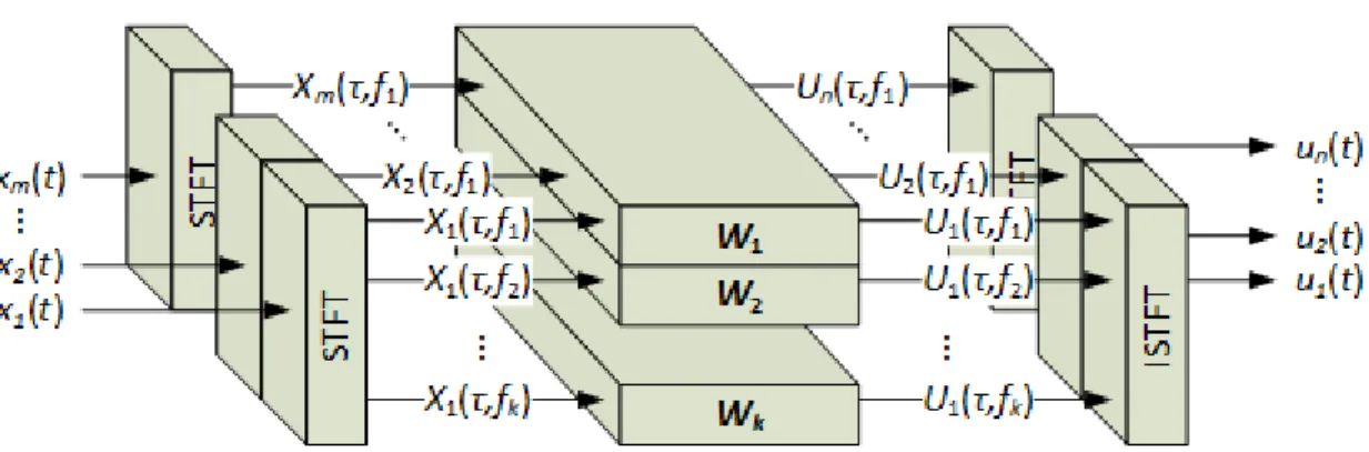
In 1998, Paris Smaragdis [27] proposed using ICA in the frequency domain to address the problem of convolutive mixing (8). Figure 3 illustrates the approach. Speech signals 𝑥𝑖(𝑡) are received from m microphones. Each signal is windowed and short-time
Fourier transformed (STFT) to produce complex coefficients 𝑋𝑖(𝜏, 𝑓) at k orthogonal frequencies. The STFT is repeated at short time intervals (𝑡𝜏−1, 𝑡𝜏] where 𝜏 =
{0,1,2, … , ∞} to produce a spectrogram for each of the m microphones such as the one shown in Figure 4.
Figure 4. Spectrogram of American-English phrase “although trees that chance to stand alone outside the groves sweep forth long curved branches producing a striking contrast to the ordinary grove form.”
Orthogonality is a property of the discrete Fourier transform (DFT). The DFT is utilized in the STFT such that the 𝑋𝑖(𝜏, 𝑓) are orthogonal along the frequency axis.
∑ {[𝑋𝑖(𝜏, 𝑓𝑎)𝑒𝑗2𝜋𝑓𝑎 𝑙 𝑘] [𝑋𝑖∗(𝜏, 𝑓𝑏)𝑒−𝑗2𝜋𝑓𝑏𝑘𝑙]} 𝑘−1 𝑙=0 = 𝛿𝑎𝑏 = { 0 if 𝑎 ≠ 𝑏 𝑘|𝑋𝑖(𝜏, 𝑓𝑎)|2 if 𝑎 = 𝑏 (40)
where 𝛿𝑎𝑏 is the Kronecker delta and 𝑋𝑖(𝜏, 𝑓) is the spectral coefficient at frequency 𝑓 of
the signal produced by the 𝑖th microphone over time interval (𝑡
𝜏−1, 𝑡𝜏]. Since the 𝑋𝑖(𝜏, 𝑓)
are orthogonal along the frequency axis, ICA can be performed independently at each frequency along the time axis to produce an 𝑛 × 𝑚 unmixing matrix Wf for each of the k
frequencies. The unmixed estimates of the 𝑛 ≤ 𝑚 sources 𝐮(𝑡) = 𝐬̂(𝑡) are obtained from separated spectrums 𝑈𝑗(𝜏, 𝑓) using the inverse short time Fourier transform (ISTFT).
2.2.1 The Short Time Fourier Transform
The short time Fourier transform gives a local spectrum of a signal whose spectrum varies with time. In continuous time, the transform is
𝑋(𝜏, 𝑓) = ∫ 𝑥(𝑡)𝑔(𝑡 − 𝜏)𝑒−𝑗2𝜋𝑓𝑡𝑑𝑡
∞
−∞
(41) where 𝑔(∙) is a window having non-zero value for a finite interval around zero and 𝑋(𝜏, 𝑓)
is a complex coefficient giving the magnitude and phase of the signal 𝑥(𝑡) at frequency 𝑓
and time 𝜏. In practice, we use uniform discrete time sampling to capture the input signal. The corresponding short time discrete Fourier transform is
𝑋(𝜏, 𝑓) = ∑ 𝑥[𝑡]𝑔[𝑡 − 𝜏]𝑒−𝑗2𝜋𝑓𝑇t ∞
𝑡=−∞
(42) where 𝑡 and 𝜏 are now integer sample indexes, 𝑥[𝑡] is the value of the 𝑡th sample of the
input signal, 𝑔[𝑡 − 𝜏] is the value of the window at sample 𝑡, 𝑓 is an integer frequency index often referred to as the frequency bin, and 𝑇 is the number of non-zero values in the window.
The choice of window is an important consideration. First, in order to accurately transform the room impulse response ℎ(𝑡) to frequency response 𝐻(𝑓), the window must be long enough to capture the many trajectories from speaker to microphone. Second, the window should not be so long as to blend phonemes (i.e. perceptually distinct units of sound that distinguish one word from another) and silence intervals together. The silence intervals between phonemes give speech its Gaussian distribution. This super-Gaussian distribution is exploited in the contrast function. Without it, there is no contrast. Figure 4 above shows the spectrogram of a 24-word American-English phrase. Phoneme
utterances are the intervals of strong harmonic content separated by short intervals of silence.
The discrete Fourier transform suffers from a phenomenon called “leakage.” This problem can be mitigated by using windows designed to shape leakage. Leakage occurs in the DFT because only frequencies that correspond to discrete frequency bins are orthogonal. Frequencies between those discrete bins project onto them (i.e. “leak” into them). Discrete frequency bins are spaced at intervals of
𝑓𝑅 =
𝑓𝑆
𝑇 (43)
where 𝑓𝑅 is the spacing between frequency bins (i.e. the frequency resolution of the DFT),
𝑓𝑆 is the sample rate in samples-per-second, and 𝑇 is the number of samples in the window.
Plots of (a) a 16-sample window of 4.0, 4.5 and 5.0 Hz sinusoids sampled at 16 samples-per-second and (b) the DFT of 4.0, 4.5 and 5.0 Hz sinusoids with 1.0 Hz resolution are shown in Figure 5. The blue 4.0 Hz sinusoid and green 5.0 Hz sinusoid transform into impulses at the ±4.0 and ±5.0 Hz frequency bins respectively. However, the red 4.5 Hz sinusoid “leaks” into all of the frequency bins.
Figure 5. Plots of (a) discrete time sampled 4.0, 4.5 and 5.0 Hz sinusoids and (b) their magnitude spectrum at 1.0 Hz resolution.
The reason for this can be seen in Figure 6. Plot (a) shows a 16 sample 1 second rectangular window and plot (b) its DFT with 0.5 Hz resolution. The Fourier transform of the rectangle window is the sinc function. Nulls can be seen at the integer frequencies, which are spaced at the reciprocal of the window length (i.e. 1 Hz) intervals. Frequencies between the nulls follow the envelope of the sinc function. Multiplication of the rectangular window by the signal is equivalent to the convolution of their transforms (𝐺 ∗ 𝑋)(𝑓).
𝑔(𝑡)𝑥(𝑡)⇔ (𝐺 ∗ 𝑋)(𝑓) = ∑ 𝐺(𝜉)𝑋(𝑓 − 𝜉)𝔉
∞
𝜉=−∞
(44) Thus any discrete frequency bin 𝑓, includes contributions from all frequencies that are not multiples of 1 Hz (i.e. the reciprocal of the window width).
0 0.1 0.2 0.3 0.4 0.5 0.6 0.7 0.8 0.9 1 -1 0 1 t (s) x ( t )
(a) Discrete Time Sampled Sinusoids
4.0 Hz 4.5 Hz 5.0 Hz -8 -6 -4 -2 0 2 4 6 8 0 5 10 f (Hz) | X ( f )|
(b) Magnitude Spectrum of Sinusoids
4.0 Hz 4.5 Hz 5.0 Hz
Figure 6. Plots (a) and (c) are discrete time samples of 1 second rectangular and Hann windows. Plots (b) and (d) are their magnitude spectrums at 0.5 Hz resolution.
On the other hand, Figure 6 (c) shows a 16 sample 1 second Hann window and (d) plots its DFT with 0.5 Hz resolution. The convolution of the signal spectrum with a Hann window’s frequency response results in contributions from only frequencies local to 𝑓
being included in frequency bin 𝑓. Thus “leakage” is not eliminated, but reshaped to provide the frequency response local to bin 𝑓. Windows have been designed to provide various main lobe widths and side lobe suppressions. The Hann window (a.k.a. raised cosine window) can be described mathematically as
𝑔(𝑡) =1
2[1 − cos (2𝜋 𝑡
𝑇)] (45)
With -18 dB per octave side lobe roll-off, the Hann window is the most popular choice in the literature [31]-[33], [35]-[38].
0 0.5 1 1.5 2 0 0.5 1 t (s) g ( t )
(a) Discrete Time Sampled Rectangular Window
-5 0 5 0 10 20 (b) DFT of Rectangular Window | G ( f )| f (Hz) 0 0.5 1 1.5 2 0 0.5 1 t (s) g ( t )
(c) Discrete Time Sampled Hanning Window
-5 0 5 0 5 10 (d) DFT of Hann Window | G ( f )| f (Hz)
2.2.2 Permutation Ambiguity
ICA in the frequency domain has advantages over time domain approaches for reverberant environments [44]. It is computationally less complex because convolutive mixtures in the time domain are transformed to instantaneous mixtures in the frequency domain. Convergence is also faster due to fewer parameters to be adjusted.
However, ICA in the frequency domain suffers from permutations in the coefficients of the demixing matrices from frequency bin to frequency bin. ICA’s estimate of the inverse of the mixing matrix is scaled and permuted
𝐖 = 𝐃𝐏𝐀̂−1 (46)
where D is a diagonal scaling matrix and P is a permutation matrix having a single unitary element per row and column and the remaining elements zero. Scaling can be controlled by normalizing the rows of W, but permutation is arbitrary. Suppose that 𝑆𝑖(𝑓) are the short time frequency coefficients of source i, and 𝑈𝑗(𝑓) are its estimates using ICA. There
is a one-to-one mapping of i to j, but i does not necessarily equal j. Furthermore, because ICA is performed independently for each frequency bin 𝑓, there is no guarantee that the
coefficients in the 𝑗th row of the demixing matrix 𝐖𝑓𝑎 produce an estimate of the same
source as those in the 𝑗th row of the demixing matrix 𝐖
𝑓𝑏 where 𝑓𝑎 ≠ 𝑓𝑏. In fact, it has
been observed that these permutations between the rows of 𝐖𝑓𝑎 and those of 𝐖𝑓𝑏 do indeed
occur. If this ambiguity in the mapping of source 𝑖 to estimate 𝑗 is not resolved, the ISTFT will produce meaningless results.
A number of solutions to this problem have been published with varying degrees of success [28]-[33]. The common factor in all of these solutions is that they take advantage
of dependency between frequency bins. Speech consists of a sequence of phonemes separated by intervals of silence. Figure 4 above demonstrates the dependency between frequency bins. It shows the spectrogram of a 24-word American-English phrase. Intervals of phoneme utterance show harmonics spanning the speech bandwidth. These phoneme utterance intervals are separated by intervals of silence. Therefore, if any frequency bin has energy, it is quite likely that many frequency bins have energy. Exploitation of this dependency led to the development of independent vector analysis, which the next section covers.
2.3 Independent Vector Analysis (IVA)
Solutions to the permutation problem of ICA in the frequency domain led researchers to view the independence of source spectrums in a different way. Rather than treating the random source variables 𝑆𝑗(𝜏, 𝑓) as independent over frequency, they exploited the
inherent dependency of speech signals over frequency and developed a class of algorithms that came to be referred to as independent vector analysis.
2.3.1 Natural Gradient IVA Algorithm
In January of 2007, T. Kim published a natural gradient IVA algorithm [35] that utilized the spherically symmetric Laplacian (SSL) multivariate source prior model
𝑝𝑆⃑
𝑗(𝑆⃑𝑗) ∝ exp (−√∑|𝑆𝑗(𝑓)|
2 𝑓
) (47)
where 𝑆⃑𝑗 refers to the discrete frequency spectrum of the 𝑗th source, which is a vector. The
speech [35]. The SSL distribution more accurately models the speech spectrogram then an independent multivariate joint Laplacian because it models the dependence of sources across frequency.
The difference between an independent multivariate joint Laplacian distribution and SSL is illustrated in Figure 7. Under the independent Laplacian distribution, conditional probabilities 𝑝(𝑠0|𝑠1) and 𝑝(𝑠1|𝑠0) have the same peaked Laplacian shape as
marginal probabilities 𝑝(𝑠0) and 𝑝(𝑠1) for all values of 𝑠0 and 𝑠1. Under the SSL distribution, conditional probabilities 𝑝(𝑠0|𝑠1) and 𝑝(𝑠1|𝑠0) only retain the Laplacian shape at 𝑝(𝑠0|𝑠1 = 0) and 𝑝(𝑠1|𝑠0 = 0). For all non-zero values of 𝑠0 and 𝑠1, the
distribution is less sharply peaked. The white curve corresponding to the conditional probability 𝑝(𝑠0|𝑠1 = 1) in each plot illustrates this point. If source spectrum coefficient
𝑠1 is non-zero, then it is less likely that source spectrum coefficient 𝑠0 is zero under the SSL distribution than it is under the independent distribution.
Kim used the SSL multivariate source prior with the natural gradient algorithm discussed in Section 2.1.3 above to maximize the independence of the estimated source spectrums 𝑈⃑⃑⃑𝑗 = 𝑆⃑̂𝑗. As with ICA in the frequency domain, natural gradient descent is
performed at each frequency on whitened and centered microphone spectrum coefficents
𝑋𝑖(𝑓) using a score function derived from the SSL prior
Δ𝐖𝑓 = [𝐈 − E{𝚽(𝑓, 𝐳)𝐳𝐻}]𝐖 𝑓, 𝐳 = [𝑈⃑⃑⃑1, … , 𝑈⃑⃑⃑𝑛] 𝑇 (48) 𝚽(𝑓, z) = [ 𝜑(𝑓, 𝑈1(𝑓1), … , 𝑈1(𝑓𝑘)) ⋮ 𝜑 (𝑓, 𝑈𝑗(𝑓1), … , 𝑈𝑗(𝑓𝑘)) ⋮ 𝜑(𝑓, 𝑈𝑛(𝑓1), … , 𝑈𝑛(𝑓𝑘))] (49) 𝜑 (𝑓, 𝑈𝑗(𝑓1), … , 𝑈𝑗(𝑓𝑘)) = 𝜕√∑𝑓𝑘 |𝑈𝑗(𝜉)|2 𝜉=𝑓1 𝜕𝑈𝑗(𝑓) = 𝑈𝑗(𝑓) √∑𝑓𝑘 |𝑈𝑗(𝜉)|2 𝜉=𝑓1 (50)
Kim found that his algorithm consistently outperformed two frequency domain ICA algorithms with permutation mitigation schemes based on interfrequency dependency [28] and interfrequency dependency combined with direction of arrival [33].
2.3.2 Fixed-point IVA Algorithm
Around the same time that Kim published his natural gradient IVA algorithm, I. Lee published a fixed-point IVA algorithm [36] using the SSL source prior. The log-likelihood function based on the SSL source prior is
𝐺(𝑈⃑⃑⃑𝑗) = √∑|𝑈𝑗(𝑓)|2
𝑓
(51) After deriving the non-linear score functions and substituting them into the fixed-point iteration (32) for one row of the demixing matrix assuming centered and spatially whitened microphone spectrums, one obtains
Step 1: 𝐰𝑗,𝑓+ = E { 1 (∑ |𝑈𝑓 𝑗(𝑓)|2) 1 2 ⁄ + |𝑈𝑗(𝑓)|2 (∑ |𝑈𝑗(𝑓)| 2 𝑓 ) 3 2 ⁄ } 𝐰𝑗,𝑓 − E {𝑈𝑗 ∗(𝑓)[𝑋 0(𝑓), … , 𝑋𝑚(𝑓)] (∑ |𝑈𝑗(𝑓)| 2 𝑓 ) 1 2 ⁄ } (52) Step 2: 𝐰𝑗,𝑓+ = 𝐰𝑗,𝑓 + ‖𝐰𝑗,𝑓+ ‖
where 𝐰𝑗,𝑓 denotes the 𝑗th row of the 𝑓th demixing matrix 𝐖𝑓. After computing all rows
for one fixed-point iteration, the rows of the demixing matrix are decorrelated using symmetric decorrelation.
𝐖𝑓 = (𝐖𝑓𝐖𝑓𝐻) −1 2⁄
𝐖𝑓 (53)
Lee also evaluated other non-linear score functions not derived from the SSL source prior. However, later research by Liang et al. [40] showed that a score function based on a spherically symmetric sparse prior delivered the best performance. We will review this research in Section 2.3.5 below.
2.3.3 IVA in Real Time
In July of 2010, T. Kim published an IVA algorithm that could be executed in real time on a low power 24-bit DSP running at only 7.68 MHz and utilizing less than 24 kB of data memory and 36 kB of program memory [38]. This is a significant result since the type of wearable that would benefit from BSS enhanced ASR will also need to conserve power. If the wearer is only one speaker of interest, but there are many microphone elements, the power saved in transmitting a single separated speech signal rather than the mixed signals from all microphone elements, may be greater than the power required to do the separation on the wearable. This would result in a net savings in total power consumption.
The natural gradient and fixed-point algorithms discussed in Sections 2.3.1 and 2.3.2 above could be done in real time using a block-wise batch approach. This approach would require buffering an ensemble of spectrums in order to compute the expectations in (48) and (52). Buffering this ensemble of spectrums would require a large amount of memory, which is antithetical to low power. Kim chose instead an online algorithm based on the natural gradient, but with a few modifications.
First, spatial whitening is a complex algorithm requiring the computation of expectations, which we want to avoid. Kim’s online algorithm uses unwhitened microphone spectrum data.
Second, the expectation in (48) is replaced by the instantaneous scored correlation
Δ𝐖𝑓(𝜏) = (𝐈 − 𝐑𝑓(𝜏)) 𝐖𝑓(𝜏),
𝐑𝑓(𝜏) = 𝚽(𝑓, 𝐳(𝜏))𝐳𝐻(𝜏),
𝐳(𝜏) = [𝑈⃑⃑⃑1(𝜏), … , 𝑈⃑⃑⃑𝑛(𝜏)] 𝑇
(54)
Third, the gradient in (54) goes to zero whenever 𝐑𝑓(𝜏) = 𝐈. However, Kim’s
algorithm does not spatially whiten the input data and uses instantaneous estimates for
𝑈⃑⃑⃑𝑗(𝜏) rather than their expectations. Therefore, a large change in average amplitude of the
spectral coefficients 𝑈⃑⃑⃑𝑗(𝜏) results in a large gradient causing the demixing matrices to
diverge. This condition occurs frequently in speech due to the silence intervals. Kim’s solution is to introduce a nonholonomic constraint [21].
Δ𝐖𝑓(𝜏) = (diag{𝐑𝑓(𝜏)} − 𝐑𝑓(𝜏)) 𝐖𝑓(𝜏) (55)
This constrains 𝑤𝑖𝑖,𝑓= 0 and prevents the rows of 𝐖𝑓 from diverging. The
constraint is nonholonomic because at any point 𝐖𝑓 in the 𝑛2-dimensional space of 𝐖𝑓,
∆𝐖𝑓 is constrained in (𝑛2− 𝑛) directions, but trajectories can reach any point in the entire
𝑛2-dimensional space.
In addition to stabilizing convergence, Kim’s constraint eliminates the need to adjust the diagonal of the demixing matrix altogether. Instead, the mixing matrix is initialized to 𝐈 and the diagonal elements remain always at unity. This is justified by the fact that scaling the rows of the mixing matrix does not change the quality of separation. As shown in (46), all scalings of the rows of 𝐖 are in fact equivalent with respect to