Forecasting Inflation in Real Time

(1)

UC Riverside

UC Riverside Electronic Theses and Dissertations

Title

Forecasting Inflation in Real Time Permalink https://escholarship.org/uc/item/9800k4tv Author Jia, Mingyuan Publication Date 2019 Peer reviewed|Thesis/dissertation

(2)

UNIVERSITY OF CALIFORNIA RIVERSIDE

Forecasting Inflation in Real Time

A Dissertation submitted in partial satisfaction of the requirements for the degree of

Doctor of Philosophy in Economics by Mingyuan Jia September 2019 Dissertation Committee:

Dr. Marcelle Chauvet, Chairperson Dr. Aman Ullah

(3)

Copyright by Mingyuan Jia

(4)

The Dissertation of Mingyuan Jia is approved:

Committee Chairperson

(5)

Acknowledgments

The past five years has been the most important and fruitful period in my life. It gets me ready to be an intellectually adequate economist. I would like to take this opportunity to express my sincere gratitude to many people for their contributions to my graduate study and research. First, I would like to thank my advisor, Professor Marcelle Chauvet, without whom this thesis would not have been possible. She not only taught me how good empirical macroeconomic research is done, but also guide me through practical issues in policy making. I appreciate all her contributions of time and ideas to make my Ph.D. experience productive and stimulating. I am grateful to the rest of my committee members, Professor Aman Ullah and Professor Dongwon Lee, for their great support and invaluable advice. Professor Lee provided me extensive personal and professional guidance and taught me a great deal about economic research, job market and academic life in general. I extend my thanks to the cohort of 2014 econ students. They are supportive in both my life and research. They are Yun Luo, Jianghao Chu, Shiyun Zhang, Hien Nguyen, Yi Mao, Taghi Farzad, Hanbyul Ryu, Deepshikha Batheja, Yoon Ro, and all the alumni who have helped me both in research and daily life.

(6)

ABSTRACT OF THE DISSERTATION

Forecasting Inflation in Real Time by

Mingyuan Jia

Doctor of Philosophy, Graduate Program in Economics University of California, Riverside, September 2019

Dr. Marcelle Chauvet, Chairperson

This dissertation is intended to model the dynamics of inflation and forecast short-run and long-run inflation using high frequency data. It first proposes a mixed-frequency unobserved component model in which the common permanent and transitory inflation components have time-varying stochastic volatilities. The key aspects of the model are its flexibility to describe the changing inflation over time, and its ability to represent distinct time series properties across price indices at mixed frequencies. More importantly, the model is applied to builds short-run and long-run coincident indicators of US inflation at the weekly frequency. The dynamics of the latent inflation factor shows that the persistence of US inflation has reduced since 1990s due to different components over time. Next, it proposes a nowcasting model for headline and core inflation of US CPI. The final selected variables include daily energy price, commodity price, dollar index, weekly gas price, money stock and monthly survey index. The model’s nowcasting accuracy improves as information accumulates over the course of a month, and it easily outperforms a variety

(7)

of statistical benchmarks. Moreover, it uses a Nelson-Siegel Dynamic Factor model to fit the monthly term structure of inflation expectation and describes its dynamics over time. The extracted inflation factors correspond to the level, slope and curvature of the term structure of inflation expectation. It shows that a decomposition of the yield curve spread into its expectation and risk premia components helps disentangle the channels that connect fluctuations in Treasury rates and the future state of the economy. In particular, a change in the yield curve slope due to expected real interest path and inflation expectation path, is associated with future industrial production growth and probability of recession.

This dissertation adds to the literature by building a mixed-frequency model that can track inflation in real time and produce better nowcasting results than the existing method, by fitting the inflation expectation with a dynamic factor model that can describe the dynamics of the whole term structure and by proving the usefulness of both inflation expectation slope and real yield spread in predicting future economic activity.

(8)

List of Figures

1.1 Extracted Weekly Inflation Index . . . 21

1.2 Estimated Inflation Indicator, CPI and PCE Deflator . . . 22

1.3 Estimated Trend Inflation and Stochastic Volatility . . . 26

1.4 Trend Inflation and Core Inflation . . . 27

1.5 Estimated Trend Inflation and Inflation Expectation . . . 28

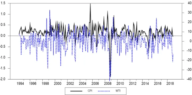
2.1 CPI Inflation and Crude Oil Price . . . 47

2.2 CPI Inflation and Dollar Index . . . 48

2.3 CPI Inflation and M1 . . . 49

2.4 CPI Inflation and Gasoline Price . . . 49

2.5 CPI Inflation and ISM Price Index . . . 50

2.6 Nowcast of MF-UCSV Model . . . 56

2.7 Nowcast of MF-DF . . . 56

2.8 Nowcast of AR Model . . . 57

3.1 Break-even Inflation and Trend Inflation . . . 67

3.2 Shape of the Term Structure of Inflation Expectation . . . 68

(11)

List of Tables

1.1 Augmented Dicky-Fuller Unit Root Test . . . 16

1.2 Autocorrelations of the First Difference of Inflation . . . 17

1.3 Factor loading Estimates . . . 23

2.1 Nowcasting Model with 5 and 6 Candidate Variables . . . 52

2.2 Nowcasting Model with 7 Variables . . . 54

2.3 Nowcast Comparison . . . 55

3.1 The Term Structure of Inflation Expectation Parameter Estimates . . . 72

3.2 Summary Statistics for Measurement Errors . . . 73

3.3 Industrial Production and Yield Spread . . . 77

3.4 Industrial Production, Yield Spread and IP Lags . . . 77

3.5 Industrial Production, Yield Spread and FFR . . . 78

3.6 Industrial Production, Expectation and Term Premium . . . 79

3.7 Industrial Production, Inflation Expectation Slope, Real Yield Slope and Term Premium . . . 81

3.8 Industrial Production, Inflation Factor,Real Term and Term Premium . . . . 82

3.9 Recession and Yield Spread . . . 83

3.10 Recession, Expectation term and Term premium . . . 84

3.11 Recession, Inflation Expectation, Real Spread and Term premium . . . 84

(12)

Chapter 1 Real-Time Indicator of Weekly Inflation

with A Mixed-Frequency Unobserved

Component Model with Stochastic

Volatility

Preview of Chapter 1

This chapter builds short-run and long-run coincident indicators of inflation at the weekly frequency. The author proposes a mixed-frequency unobserved component model in which the common permanent and transitory inflation components have time-varying stochastic volatility (MF-UCSV model). The key aspects of the model are its flexibility

(13)

to describe the changing inflation over time, and its ability to represent distinct time series properties across price indices at mixed frequencies. The model is estimated using Bayesian Gibbs Sampler and data on weekly commodity inflation, monthly consumer inflation, expenditures inflation, and quarterly GDP deflator inflation. The empirical results show that the constructed weekly inflation indicator closely matches monthly consumer and expenditure inflation. Additionally, the paper proposes and estimates a measure of high frequency trend inflation, which are in line with survey forecast and core inflation, and provides alternative to existing trend measures. We also study the changing persistence of inflation, and find that although it has reduced since the 1990s, it was due to different components over time. Interestingly, we also find that inflation volatility increased during the Great Recession, but this did not change the mean-reversion property of inflation. Overall, the model provides a strategy for real-time multivariate tracking and nowcasting of inflation at the weekly frequency, as new data are released.

1.1 Introduction

Inflation is one of the most watched economic series by policymakers and the public in general. Monetary policymakers continuously monitor inflation releases to update their expectation about future economic conditions and to control price stability. Market practitioners also rely on inflation reports in forming expectations when negotiating long-term nominal commitments. There is a growing recent literature on rich data environment

(14)

(large datasets) and mixed frequency framework that has yielded major advances in assessing real economic activity, nowcasting, and forecasting output. However, this method has not been extensively applied to study inflation dynamics. Building an inflation indicator based on a set of variables is challenging given the important time-varying properties of inflation.1 This is especially the case across price indices at different frequencies. Aruoba and Diebold (2010) construct a real-time monthly inflation indicator with the same framework used in Aruoba, Diebold and Scotti’s (ADS, 2009) business condition indicator. However, the model does not provide a characterization of changing inflation dynamics, in particular, the evolving local mean and time-varying volatility.

This chapter proposes a framework with underlying trend and cycle components representing long- and short-run inflation dynamics, which are used to construct high frequency coincident indicators of inflation. The proposed model encompasses price measures sampled at different frequencies, including weekly, monthly and quarterly price indices. The output is estimated weekly inflation indicators, which depict historical inflation trend and cycle, and that can be used to assess current inflation in real-time. The possibility of a high frequency inflation indicator providing more timely measurement than the official publication is very appealing. Official inflation measures can only be observed at the monthly frequency and with publication lags. For example, U.S. CPI is announced at the middle of the month for measures of inflation for the month prior.

The increasing availability of data at higher frequency has sparked interest in mixed

(15)

frequency models. On one hand, mixed-frequency factor model and MIDAS (mixed-data sampling) model have become important tools for nowcasting and forecasting, using daily or weekly time series. Monteforte and Moretti (2013), Modugno (2013), Breitung and Roling (2014) examine the predictability of commodity prices and asset prices with this framework. On the other hand, researchers from other fields such as computer science and statistics have advanced methods to study high frequency data. With the recent large data set collected by electronic commerce system, such as Amazon, Walmart in the U.S. or Alibaba in China, among many others, daily price information is extracted and aggregated in few minutes using web crawler technology.2 These measures are gradually accepted by private agents to complement the official inflation publications. However, the existing methods (e.g. machine learning) are designed to predict but not to obtain inferences regarding time series dynamics. In particular, the data collecting and filtering approaches that are used by high frequency price indices (e.g. online price index and commodity price index) are distinct from those that are used by official statistical agencies, and a formal statistical treatment of inflation dynamics at high frequency is still lacking.

Our approach involves formal modeling of inflation dynamics characterizing its trend, cycle, and volatility, while allowing for mixed-frequency. In particular, this paper proposes a mixed frequency small-scale unobserved component factor model with stochastic

2_{For e.g. The Billion Prices Project (BPP) operated by MIT Sloan and Harvard Business School use big}

data to estimate dynamics in prices and implications for economic theory. This project uses prices collected from hundreds of online retailers on a daily basis to build inflation index and already has been applied to measure Argentina’s inflation. In China, the companies Alibaba and Tsinghua University are collaborating to publish a daily internet-based consumer price index (icpi). This project not only provides the aggregate price index, but also price indices in sub-categories.

(16)

volatility - the MF-UCSV model. In the proposed model, underlying inflation process is approximated as a sum of unobserved common permanent and transitory factors. The permanent component captures long-run trend inflation, while the transitory component captures short-run deviations of inflation from its trend value. Additionally, the variances of the permanent and transitory disturbances are allowed to evolve over time according to a stochastic volatility process. Thus, the persistence of the inflation process is summarized by the relative importance of the variability of permanent and transitory components. The key aspects of the model are its flexibility to describe the changing inflation over time, and its ability to represent distinct time series properties across price indices at mixed frequencies. Price measures differ in terms of data collecting process, categories, utilization, but are highly correlated and may be driven by a set of common latent factors. The proposed flexible model allows for the potential distinct dynamics of underlying inflation, and also extracts common trend and common cyclical movements across the series. The underlying inflation indicators are extracted from a set of weekly, monthly, and quarterly price indices. The results indicate that the weekly inflation index tracks historical inflation dynamics well in the sense that it successfully identifies important inflation cycle and trend phases, including their severity and duration. Additionally, the estimated inflation indicator closely matches monthly consumer and expenditures inflation at the weekly frequency in real-time. Overall, the model provides a strategy for real-time multivariate tracking and nowcasting of inflation as new data are released. In particular, the real-time trend inflation estimates are in line with survey forecast and core inflation, which provide alternative to existing trend

(17)

measures.

This chapter has several contributions to the literature. To our knowledge, this is the first one that builds high frequency short-run and long-run U.S. inflation coincident indicators that can be updated in real-time. Previous works do not use high frequency data or do not use them to build coincident indicators. Aruoba and Diebold (2010) build a U.S. inflation indicator but based on monthly and quarterly series. Similar to Aruoba and Diebold (2010), Modugno (2013) uses a dynamic factor model with three factors corresponding to weekly, monthly and quarterly series to forecast U.S. Consumer Price Index and Harmonised Index of Consumer Price for the Euro Area. Monteforte and Moretti (2013) use MIDAS regression framework with daily data to forecast inflation. However, these papers do not construct a short-run and long-run coincident indicators of inflation as proposed here.

Second, the MF-UCSV model takes into account potential nonstationarity in inflation dynamics. Many researchers suggest models that take account of slow-varying local mean for inflation perform reasonably well in forecasting inflation. Atkeson and Ohanian (2001) show that forecasts from simple random walk model cannot be statistically beaten by alternatives. Following their work, Stock and Watson (2007, 2016) proposed characterization of quarterly rate of inflation as an unobserved component model with stochastic volatility. Faust and Wright (2013) compare various inflation forecasts and find that models based on stationary specifications for inflation do consistently worse than non-stationary models. However, the related literature that focuses on extracting inflation

(18)

indicator (Diebold and Aruoba, 2010) or nowcasting (Giannone, et al. 2006) with mixed frequency framework are all based on stationary specifications for inflation. This raises the question on whether the consideration of nonstationarity in these frameworks could also improve characterization of the dynamic properties of latent inflation. For example, the temporal aggregation of latent autoregressive factor is also autoregressive, while the GDP deflator inflation is better approximated as integrated moving average. In our framework, the factor loading along with changing volatilities can solve this problem by providing appropriate approximation for each series. Our mixed frequency MF-UCSV model takes into account nonstationarity and yields an estimated trend inflation at high frequency. Trend inflation is an important tool for monetary policy as it conveys information on long run inflation expectations.

Finally, filtering out the noise in multiple inflation measures has not been done in the mixed frequency literature. Generally, there are two approaches in the literature to approximate trend inflation. Clark (2011), Faust and Wright (2013), among others, use measures of long-run inflation expectations from surveys forecasts (either Survey of Professional Forecasters or Blue Chip) to capture trend inflation. Survey-based trend leads to an improvement in the accuracy of model-based forecasts (see, e.g., Ang, et al. 2007). However, surveys of inflation expectation can not be replicated as it is a result of a combination of many objective (models) and subjective information. Alternatively, a range of studies has modeled trend inflation as an unobserved component (e.g. Stock and Watson 2007, Cogley and Sbordone 2008, or Mertens 2011). In this chapter, we follow

(19)

this approach, using time series smoothing methods to extract trend inflation, which is additionally obtained from a multivariate framework. The use of factor model mitigates the problem of estimating weights separately and downweighting sectors that may have large variations over time.

This chapter is organized as follows. The model is described in section 2, along with the estimation method, which uses the Gibbs Sampler used for simulating the posterior distribution of the parameters. The third section presents and interprets the empirical results. The conclusion are discussed in the fourth section.

1.2 The Model

1.2.1 The Underlying Inflation Process

Following Stock and Watson (2007), inflation is characterized by an unobserved component model with stochastic volatility. We assume that the underlying inflation process evolves daily. This assumption can be adjusted to other frequencies, like weekly or monthly.

Let πt denote the underlying inflation at dayt, which evolves following a stochastic

process:

πt =τt+ηt (1.1)

whereτtrepresents the permanent component of underlying inflation andηt represents the

(20)

equation (2):

τt =τt−1+στ,tετ,t (1.2)

and transitory component has a finite order AR(p) representation:

Φ(L)ηt=ση,tεη,t (1.3)

where functionΦ(L)is a finite lag polynomial with orderp, and has all the roots outside the

unit cycle, ετ,t and εη,t are mutually independent i.i.d. N(0,1) stochastic processes. στ,t

and ση,t represent the variability of innovations to permanent component and transitory

component. They together determine the relative importance of random walk disturbance. To model the changing volatility of inflation components, it is assumed that their log-volatility follows a random walk with no drift,

ln(σ_τ2_,_t) =ln(σ_τ2_,_t₋₁) +ντ,t (1.4)

ln(σ_η2_,_t) =ln(σ_η2_,_t₋₁) +νη,t (1.5)

where ντ,t ∼N(0,σν τ2 ) and ντ,t ∼N(0,σν η2 ). The magnitudes of time variation in στ,t

and ση,t depend on the variances of ντ,t and νη,t. In particular, a large σν τ2 means the

variability of trend components can undergo large period changes, which affect the inflation persistence indirectly.

(21)

1.2.2 Unobserved Component Model

A vector of price measures and other variables displaying comovement is modeled to depend on the latent permanent and transitory inflation factors. The daily economic variable is a linear combination of daily common permanent and transitory components. Letyi_t denote theithdaily price measures at dayt and we have below the relationship:

yi_t=βiτt+γiηt+uti (1.6)

where ui_t _∼ N(0,σ_u2_i) are contemporaneously and serially uncorrelated innovations that

capture idiosyncratic shocks to the specific price measures. βiandγiare the factor loadings

on the common permanent and transitory components.

In the mixed frequency framework, the relationship between the observed data and daily variables need to be specified. Most of the economic variables are observed at lower frequency, for example, CPI inflation and GDP inflation are monthly and quarterly measures respectively. Inflation measures growth rate of price level, then relationship between observed inflation series and underlying daily variables depends on the temporal aggregation of price index. Here we approximate the price index observed at low frequency as the systematic sampling of the daily variables, i.e. end of period value. Thus, the inflation measures can be processed as flow variable.3 Our approximation method is different from the commonly used method for approximating GDP growth rate in Mariano

3_{A comprehensive description of temporal aggregation of flow and stock variables can be seen in Aruoba,}

(22)

and Murasawa (2003). Their method is doable but will complicate our model in high frequency, by making the state variable extremely large and computation unattainable. In contrast, our approximation can cast the model into a linear form. Let ˜yi_t denote the

ith observed flow variable in low frequency. Then ˜y_ti is the intra-period sums of the corresponding daily values,

˜ yi_t =         

∑D_j=0i−1yi_t₋_j i f ytican be observed

NA otherwise (1.7) =         

βi∑D_j=0i−1τt−j+γi∑D_j=0i−1ηt−j+ut∗i i f ytcan be observed

NA otherwise

where Di is the number of days per observational period. For example, Di for monthly

CPI of January equals 31. u∗_ti adds up the daily white noise disturbances and thus follows

MA(D_i−1)process. Here we can appropriately treatu∗_tias white noise following Aruoba et al. (2009).

Following Harvey(1990), we apply the accumulator variables to handle temporal aggregation. This could greatly reduce the state of the system. LetC_τ_,_t andC_η_,_t denote the permanent and transitory component accumulator:

(23)

C_τ_,_t = θtCτ,t−1+τt (1.8)

= θtCτ,t−1+τt−1+στ,tετ,t

C_η_,_t = θtCη,t−1+ηt (1.9)

= θtCη,t−1+Φ(L)ηt−1+ση,tεη,t

whereθt is an indicator variable which is defined as:

θt =         

0 I f t isthe f irst day o f the period

1 otherwise

Then equation (7) can be written as:

˜ yi_t =          βiCτi,t+γiC i η,t+u ∗i t i f yt can be observed NA otherwise

1.2.3 State-Space Form

(24)

Yt =C 0 tαt+wt (1.10) αt+1=Atαt+Rtvt (1.11) Λt+1=Λt+ζt (1.12) w_t∼N(0,H), v_t ∼N(0,Q_t) (1.13) ζt∼N(0,W) (1.14)

where Y_t is an N×1 vector of observed variables with missing values. State vector

αt includes 8 state variables, wt and vt are Gaussian and orthogonal measurement and

transitory shocks. The time-varying variance matrixQ_t is a diagonal matrix with elements ofσ_τ2_,_t andσ_τ2_,_t. Λt is the vector of unobserved log-volatilities, andW is a diagonal matrix

containing the variance of log-volatility disturbances.

There are two special cases nested in our model. First, the changing volatility crucially depend on the covariance matrixW. When we setW =0, Λt is constant, then we return

to the normal mixed-frequency dynamic factor model. In this case, Kalman filter and smoother can be used to extract the state variables and the corresponding state disturbances. The algorithm is classical Kalman filter in the textbook. Second, instead of shutting off the stochastic volatility, we may assumeσ_τ2_,_t =σ_η2_,_t and reduce the dimension ofW to unity.

This is the case of common stochastic volatility. Koopman (2004) propose a method using importance sampling and Kalman filter to estimate the model. These two models can be

(25)

estimated by maximizing the log likelihood function. For our model with great flexibility in setting the conditional variance, MLE is not feasible.

1.2.4 Estimation

We use Bayesian MCMC method with Metropolis-within-Gibbs sampler to estimate our model. The estimation procedure, model identification, and priors will be described briefly, and more details can be obtained in the appendix.

Sampling of the parameters, including latent factors and volatilities, can be proceeded in several steps. First, since the model can be cast into state-space form, the unobserved state variablesτtandηtcan be easily drawn using Kalman smoother (Koopman and Durbin,

2003). Second, conditioning onαt andYt, elements inCt0andH can be drawn row by row

in equation (10). Taking the ithmeasurement equation ˜yi_t =βiCiτ,t+γiCηi,t+ut∗i, we can

draw the βi, γi and variance of u∗_ti following the conventional method for linear model.

Third, equation (11) can be broken down to equation (3), which is AR(p) model with heteroscedastic disturbance. Dividing byση,t, one can obtain a standard linear regression

model and draw the AR coefficients from the conjugate normal distribution. Forth, we use Jacquier, Polson, and Rossi (1994)’s algorithm and Kim, Shephard and Chib (1998)’s Metropolis rejection method to draw the stochastic volatilities, which are the unobserved components in equation (12). Fifth, conditional on the log-volatilites, σ_{ν τ}2 and σ_{ν η}2 in

(26)

1.3 Empirical Application

1.3.1 Data

The empirical application uses weekly GSCI commodity price index, monthly CPI-all items, monthly personal consumption expenditure deflator, and quarterly GDP deflator. The inflation measures are observations on 100 times first difference of the logarithm of each price indices. The sample ranges from 1970/02/01 through 2016/12/31. The extracted inflation indicator can be updated weekly, by including the high frequency commodity price index GSCI inflation (Goldman Sachs Commodity Index). GSCI index is a weighted future prices that almost covering all the sectors of commodities. It is published by Standard and Poor’s and recognized as a leading measure of general price movements in the global economy. In this paper, the daily GSCI is averaged to build our weekly GSCI index. Similar high frequency indices include daily CRB index (Commodity Research Bureau Index) which is calculated by Commodity Research Bureau, World Market Price of Raw Materials (RMP) produced by OCED and other energy prices. The commodity price index is obtained from Global Financial Data, and all other price measures are from FRED Economic Data.

We choose the data set for the following reasons. First, a small-scale factor model is sufficient to achieve our goal and illustrate the implementation of our model. Second, we only use data up to weekly frequency since daily observations are far too noisy. Third, the indicators are all price measures that assess the change of inflation from different aspects. The choice of the variable set can also be extended beyond, for example, asset prices,

(27)

Table 1.1: Augmented Dicky-Fuller Unit Root Test 1970 to 1983 1984 to 2016 1970 to 2016 GSCI inflation -24.13 -42.021 -48.727 CPI inflation -1.861 -4.823 -1.914 PCE infaltion -1.578 -3.06 -1.722 GDP Deflator inflation -2.57 -3.816 -2.23

Note: The ADF test includes a constant. The number of lags is chosen based on SIC criteria.

monetary base and survey data. These variables have some predicative power for future rate of inflation, thus sometimes are used in the literature. However, correlations between those variables and inflation are weak, which may disturb our signal extraction. So we exclude them in our estimation.

Examination of our data indicates our model is an appropriate approximation to different inflation measures. First, we use the Augmented Dickey–Fuller (ADF) test to examine the stationarity of the series. The test is done for three sample ranges: 1970 to 1983, 1985 to 2016 and the full sample period 1970 to 2016. The first sample period corresponds to the Great Inflation, while the second sub-sample includes Inflation Stabilization period when both the level of inflation and the volatility declined dramatically. The ADF test in Table 1.1 suggests a unit root in pre-1984 period and the full sample period for low frequency inflation measures (monthly and quarterly). However, the null hypothesis of unit root in the post-1984 period is rejected. This may suggest that innovations of transitory component tend to play a greater role in the inflation process.

(28)

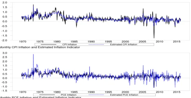
Table 1.2: Autocorrelations of the First Difference of Inflation 1970 to 1983 1984 to 2016 1970 to 2016 lags 1 2 3 1 2 3 1 2 3 GSCI inflation -0.513 0.008 0.032 -0.476 -0.006 -0.011 -0.523 0.013 0.042 CPI inflation -0.461 0.12 -0.111 -0.158 -0.294 -0.080 -0.267 -0.153 -0.085 PCE inflation -0.336 -0.048 -0.099 -0.233 -0.226 -0.059 -0.264 -0.175 -0.068 GDP inflation -0.219 -0.103 -0.031 -0.404 -0.066 -0.009 -0.303 -0.074 -0.029

Second, equation (1) to (3) imply that the first-order autocorrelation is negative for the first difference of inflation. Table 1.2 presents estimated autocorrelation for the change in inflation over three sample periods. The first-order autocorrelation is negative for each of the measures in all sample periods. For GDP inflation, ∆πt is negatively correlated, with

the first autocorrelation much larger in absolute magnitude in the second period than the first.

1.3.2 Model Implementation

We assume that the transitory component follows AR(1) process. Modeling the persistence with AR(1) process would be inadequate, high-order dynamics nevertheless is not statistically better, as the transitory shock would decay too quickly when we assume the latent factors evolve daily.

(29)

            ˜ yGSCI t ˜ yCPI_t ˜ yPCE_t ˜ yGDPD_t             =             0 0 β1 γ1 0 0 0 0 0 0 0 0 β2 γ2 0 0 0 0 0 0 β3 γ3 0 0 0 0 0 0 0 0 β4 γ4                                         τt ηt CW τ,t CW_η_,_t CM_τ_,_t C_ηM_,_t CQ_τ,t CηQ,t                             +             uGSCI t uCPI_t u_tPCE uGDPD_t             , (1.15)                             τt ηt CW_τ_,_t CW_η_,_t C_τM_,_t C_ηM_,_t CτQ,t C_ηQ_,_t                             =                             1 0 0 0 0 0 0 0 0 φ 0 0 0 0 0 0 1 0 θtW 0 0 0 0 0 0 φ 0 θ_tW 0 0 0 0 1 0 0 0 θ_tM 0 0 0 0 φ 0 0 0 θ_tM 0 0 1 0 0 0 0 0 θtQ 0 φ 0 0 0 0 θtQ                                                         τt−1 ηt−1 CW_τ_,_t₋₁ CW_η_,_t₋₁ C_τM_,_t₋₁ C_ηM_,_t₋₁ C_τQ_,_t₋₁ CQ η,t−1                             +                             1 0 0 1 1 0 0 1 1 0 0 1 1 0 0 1                                 vτ,t vη,t     , (1.16)             uGSCI_t uCPI_t uPCE_t u_tGDPD             ∼N(04×1,H),     vτ,t vη,t     ∼N(0,Qt),

(30)

H=             σ₁2 0 0 0 0 σ₂2 0 0 0 0 σ₃2 0 0 0 0 σ₄2             , (1.17) Qt=     στ2,t 0 0 ση2,t     , (1.18)     ln(σ_τ2,t) 0 0 ln(ση2,t)     =     ln(σ_τ2_,_t₋₁) 0 0 ln(σ_η2_,_t−1)     +     ντ,t νη,t     , (1.19)     ντ,t νη,t     ∼N(0,W), W=     σ_{ν τ}2 0 0 σ_{ν η}2     . (1.20)

We identify the model and set the prior hyperparameters in the following ways: First, we restrict the factor loadings β4 and γ4 to be 1 to identify the scale of factor loadings

and of the unobserved components (See equation (15)). Then, we obtain the initial guess value of βi , γi , φ and σi as estimates of the state-space model using MLE with

time-invariant variability of state disturbances. Along with factor loadings, the initial guess of the latent state variables in αt can also be estimated. Second, for the initial guess of

time-varying volatilities σ_τ2_,_t and σ_η2_,_t, we estimate a GARCH(1,1) model to obtain the

conditional variance. Third, the prior distributions ofβi,γiandφ are conjugate independent

(31)

we impose independent inverse gamma with degrees of freedom to 1 forσiinH,σν τ2 and

σ_{ν η}2 inW. Finally, following Del Negro and Otrok (2008), we fix the initial condition of stochastic volatility to zero.

1.3.3 Empirical Result

Inflation Indicator and Factor Loading

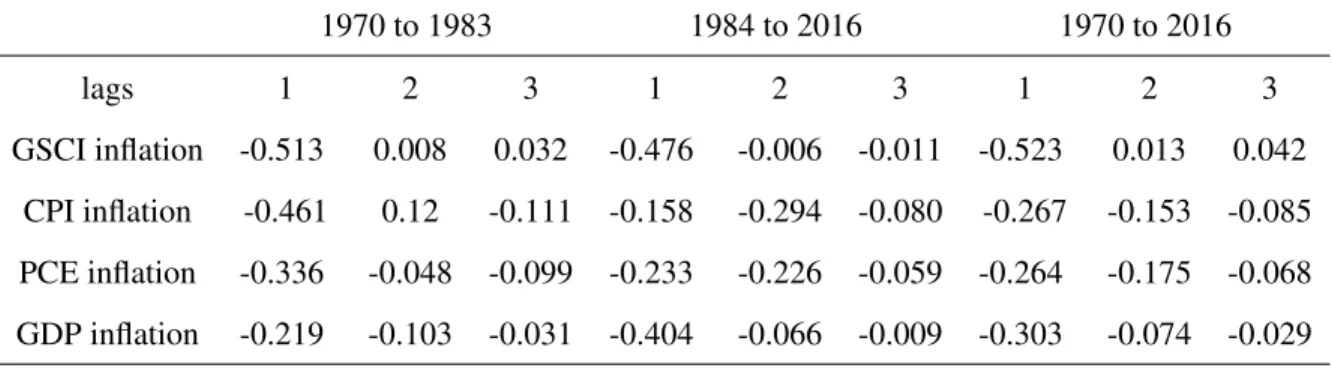
We build the coincident inflation indicator as the sum of latent permanent component and transitory component. The extracted weekly inflation indicator is plotted in Figure 1.1.4 Several observations and desirable properties are noteworthy: First, our estimated inflation indicators are available at high frequency, whereas the monthly CPI and PCE inflation are released only monthly and with weeks of lags. Therefore, our inflation indicator can be applied to nowcast CPI and PCE inflation.

Second, our inflation indicator broadly coheres with the dynamics of inflation in the past 50 years. The Great Inflation in 1970s is apparent, along with the inflation stabilization staring from 1982. The average annual inflation indicator is 6.3648 during 1970s, compared with an average value of 2.3418 after 1982 in our estimation. For the Great Inflation, we find the first peak occurred on October 6, 1974 with a weekly indicator value of 0.199632, and the second peak was on November 30, 1980, with an indicator value of 0.188673. The recent 2007 recession experienced unprecedented price decline. However,

4_{The estimated inflation factors follow daily evolution. But information of price comes on Friday of each}

week as assumed in our model, so we aggregate the daily inflation factors to get the weekly inflation index as plotted. By doing so, we can mimic the real time updating of inflation index.

(32)

Figure 1.1: Extracted Weekly Inflation Index

Note: The weekly inflation indicator is the weekly sum of the daily inflation factors.

this deflation was quite brief and lasted two months from 10/26/2018 to 01/04/2019. In addition, the estimated inflation indicator also indicates varying volatility of inflation, which is consistent with the observations in the literature (Stock and Waston, 2007). We will examine this property in the later sections with estimated conditional volatility.

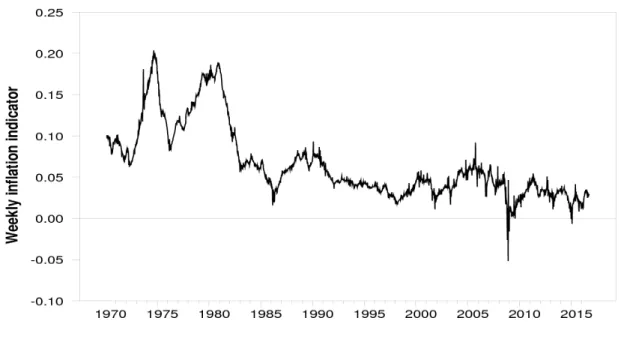
Third, our inflation indicator coheres with consumer inflation and expenditure inflation but plays no leading role in identifying the turning points. Figure 1.2 graphs the weighted inflation indicator along with monthly CPI inflation and PCE inflation. The fact that the weekly inflation indicator has no leading performance can be explained in two ways. On one hand, commodity price is made up of commodity future contracts, thus may convey limited leading information in the consumer and personal expenditure inflation. On the other hand, monthly indicators account for a large part of the extracted inflation factor as

(33)

Figure 1.2: Estimated Inflation Indicator, CPI and PCE Deflator

Note: The upper graph shows estimated monthly trend inflation along with CPI inflation; the lower one shows estimated monthly trend inflation along with PCE inflation.

indicated by the values of the factor loading. It is not surprising that the weekly inflation indicator tracks monthly consumer and personal expenditure inflation well. Adding leading variables such as term premium and M2 may improve the leading performance of our indicator.

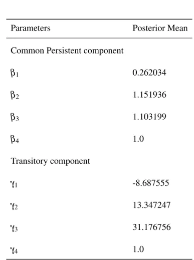
Estimated factor loadings measure the sensitivity of input variables to latent permanent and transitory components. The full sample posterior mean estimates of the factor loadings are reported in Table 1.3. The relative importance of our chosen indicators is given by the full sample posterior mean estimate of the factor loadings. For the common trend component, the monthly inflation indices have the highest posterior means, and followed by the quarterly GDP inflation. The weakest contribution comes from weekly commodity inflation (0.26). This suggests that commodity inflation is less persistent and thus few of

(34)

the variation itself are from the variation of common persistent component.

Table 1.3: Factor loading Estimates

Parameters Posterior Mean Common Persistent component

β1 0.262034 β2 1.151936 β3 1.103199 β4 1.0 Transitory component γ1 -8.687555 γ2 13.347247 γ3 31.176756 γ4 1.0

Note: β1 and γ1 are the factor loadings on GSCI commodity inflation; β2 and γ2 are the

factor loadings on CPI inflation; β3 and γ3 are the factor loadings on PCE inflation; β4

andγ4are the factor loadings on GDP deflator inflation. The estimated AR coefficient in

equation (3) is -0.69.

Among inflation measures at different sampling frequencies, monthly CPI and PCE inflation capture both the persistent and transitory components well, comparing with

(35)

quarterly inflation index in extracting low frequency movements and with weekly commodity inflation in modeling high frequency variations. This may suggest that transitory shocks in general price level vanish within a quarter. Thus, using quarterly average of inflation may overrate the model implied persistence of inflation either in univariate time series model or multivariate VAR model and New Keynesian model.

Trend Inflation and Volatilities

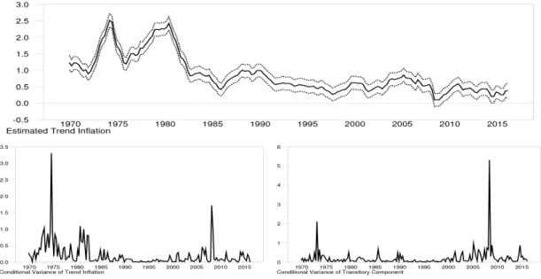
The model provides a measure of trend inflation. Figure 1.3 plots the full sample posterior means of τt , στ2,t and σ

2

η,t. The estimated trend inflation is quite smooth and

shows substantial variation over time. Trend inflation declined continuously over the two decades. Regarding the recent 2007-2009 recession, trend inflation did not plunge deeper and go under zero line, but recovered steadily to the Fed inflation target. Compared with inflation indicator which indicates a short period deflation, trend inflation only suggests a pressure of disinflation. Therefore, the decline of price in 2008 was more likely due to a one-time large shock which decayed very quickly.

There are important similarities betweenσ_τ2_,_t andσ_η2_,_t, most notably the larger variation

in 1970s coincided with high trend inflation, and persistently low volatility in 1990s followed by a remarkable increase in early 2000s. Stock and Watson (2007) suggest the recent rise of volatility as the potential reason for the decreased forecastability of inflation in recent decades. However, there are also differences between the changes in these two series. In 1990s, volatility of permanent component decreased strikingly compared to

(36)

1980s and 1970s, whereas there was only slight decrease in the volatility of transitory component. During 2000s, the volatility of both permanent and transitory components increased, but transitory component increased much more than permanent component. The persistence of inflation which depends on the relative importance of the variances of the permanent and transitory innovations is also examined. The change in inflation indicator has a negative first-order autocorrelation which summarizes the persistence of inflation process (Cecchetti, et al. 2007). The analytical expression can be calculated as:

ρ_∆_π =Cov(∆πt,∆πt−1) Var(∆π_t2) = − 1−φ 1+φσ 2 η,t σ_τ2,t+1+2φσ 2 η,t (1.21)

Note thatρ∆π has a range that depends on the AR coefficientφ. With the estimated value,

the closer it is to -0.845, the less persistent the inflation process is. Additionally, the higher

σ_τ2_,_t is relative to σ_η2_,_t, the closer inflation is to a pure random walk, and the closer the

first-order autocorrelation of∆πt is to zero. By contrast, whenσ_η2_,_tis dominant, inflation is

close to a stationary AR process. From our estimation of the weekly inflation indicator,ρ∆π

decreased by 74.12% from 1970s to the current decade. Alternatively, when inflation does change unexpectedly, how much of the surprise should we assume to be part of the new trend? We calculate the share of inflation surprise that the model currently attributes to the new trend. In our estimation, 54% of the unexpected inflation change assumed to be part of a new trend in 1970s, and this share decreased to 22% in 1990s and 19% in current decade. Overall, inflation persistence has reduced since the 1990s, but due to different components

(37)

over time. In this period with a lower persistence, inflation tended to revert to a stable trend during the 2000s, whereas in the 70s and 80s the trend moved to track inflation.

Figure 1.3: Estimated Trend Inflation and Stochastic Volatility

Note: The upper graph shows the weekly trend inflation; the lower left graph depicts the stochastic volatilies of persistent component; the lower right graph depicts the stochastic volatilities of transitory component of inflation.

Comparing with univariate model using quarterly data, our model tends to overrate the role of high frequency variations. This is shown in the higher contribution of transitory innovations to the variability of inflation process. It is not surprising that quarterly data filter out the high frequency innovations due to temporal aggregation. In contrast, weekly data highlights the volatile movements in commodity inflation, thus assign higher weights

(38)

Figure 1.4: Trend Inflation and Core Inflation Note: Trend inflation are monthly trend inflation component .

to them in signal extracting process (See Table 3 the factor loadings). Modeling transitory components as autoregressive process rather than white noise also weight more on the variability of transitory shocks.

Our model hinders the smoothness to stochastic volatility. The two spikes in 1974 and 2008 are more likely to be occasional large jumps in inflation. The 1974 spike was due to the oil crisis, and the2008 spike was due to the recent financial crisis. Hence it is possible that 2007 recession can be viewed as a temporary period with a high level of volatility in a longer period when moderate volatility is the norm.

Figure 1.4 compares model implied trend inflation with core inflation (CPI and PCE). Our trend estimates are broadly in line with the alternative measures of trend inflation. They together reflect the common low frequency variability in inflation series. However,

(39)

Figure 1.5: Estimated Trend Inflation and Inflation Expectation

Note: Long-term inflation expectation is measured with Survey of Professional Forecasters 10-years inflation expectation.

there are important differences between trend inflation and distinct core inflation measures. Core CPI inflation is much persistently higher than trend inflation and core PCE deflator during late 1970s and early 1980s, which indicates that sectors in CPI categories besides food and energy also contribute to large short-term variations.

Figure 1.5 plots our model implied trend inflation along with the median 10-year ahead forecast that has been reported in the Survey of Professional Forecasters since 1991. Trend inflation lines up with the survey forecasts but lies below trend inflation during 1990s and the current decade. The reason is that survey forecasts are always upward biased. Especially, long-term forecasts of PCE inflation from the SPF have often been a bit higher than long-term projections from the FOMC. After a slightly decline together in 1990s,

(40)

survey forecasts kept stable henceforth while trend inflation became volatile. Although many concerns disinflation due to large output gaps and unemployment in 2004 and 2008 (Williams, 2009), the substantial increase in expectations anchoring mute these pressures and revert the trend to local mean.

A subtle feature in Figure 5 is that the model implied trend inflation leads long-run survey forecast movements. This is especially obvious for the drop around 1997 and the decline after 2012. This raises the question of how inflation expectation reacts to the changes in trend inflation. A simple linear regression between one-year ahead inflation expectation and trend inflation indicates that there exists statistically significant evidence that trend inflation help forecasting trend inflation expectation. This suggests a rise of inflation that is not accompanied by a rise of inflation expectations is less likely to persist.

1.4 Summary of Chapter 1

This article introduces a mixed-frequency unobserved component model with stochastic volatility and estimate the model using Bayesian Gibbs Sampler. MF-UCSV model provides a flexible mixed-frequency framework for extracting high frequency inflation indicator, estimating trend inflation, and describing persistence of inflation. Inflation indicator and trend inflation could be flagged in the real-time as new data are released. The framework allows ragged-edge data, publication lags and non-synchronization in real time monitoring and nowcasting.

(41)

Our paper supports the desirability of using models that account for a slowly-varying trend. The changing time series properties of inflation imparts the forecasting performance of most univariate and activity-based inflation forecast (Stock and Watson, 2007). Apart from accounting for local mean and varying volatility in this paper, one could also apply methods that take account of parameter instability, such as time-varying coefficients VAR by Cogley and Sargent (2005). It is noteworthy that researches which impose a structural break also do well in some specific models (Goren, et al., 2013). However, our initial try of a regime switching model fails to detect a structural break endogenously. One possibility is that high frequency data contains too many noises which can largely disturb the inference of Markov Switching model.

Compared with the conventional way of modeling low-frequency movement from quarterly data and high frequency variations from daily or weekly data separately, we estimate the variability of both components jointly. However, our model underrate the transitory innovation due to the quickly decay in transitory dynamics. This suggests a mixed frequency model with monthly and quarterly observations should be a future research direction to examine the relative importance of transitory components.

(42)

Chapter 2 Nowcasting Headline Inflation

Preview of Chapter 2

Nowcasting contemporaneous inflation using high frequency data is difficult. This chapter proposes a mixed frequency unobserved component model for nowcasting headline inflation of consumer price index (CPI). The model is a small-scale factor model that relies on relatively few variables. These variables are sampled at different frequencies and are selected based on the forecasting performance in real time. The final selected variables includes daily energy price, commodity price, dollar index, weekly gas price, money stock and monthly survey index. The model’s nowcasting accuracy improves as information accumulates over the course of a month, and it easily outperforms a variety of statistical benchmarks. In particular, the nowcasting model outperforms the existing nowcasting models that ignore slowly moving local trend and stochastic volatility of inflation.

(43)

2.1 Introduction to Nowcasting Inflation

The annual inflation rate has been below the Fed’s target for a long time in spite of the tight labor market since 2009. In view of this situation, broad discussion concerning the current 2% inflation targeting strategy has been generated among policy makers and researchers. One popular viewpoint in the 2019 Monetary Policy Forum held by Chicago University Booth School of Business is that the Fed should adopt a symmetric 2% inflation target, or define a range of inflation between 1.5% and 3%. In particular, Fed could set a medium-term goal within that range, and revisit it periodically to take account of the changing economic circumstances. Under an inflation targeting scenario, either with an explicitly announced target or a defined range, monitoring of the inflation path plays a fundamental role in assessing policy effectiveness. The goal of this chapter is to provide early nowcasts of monthly inflation that can be useful to inform monetary policy and market practitioners. The seminal work of Giannone, Reichlin and Small (2008) is the starting point of a large literature that utilizes the high-frequency data to forecast the present condition of the economy. Accordingly, nowcasts of monthly inflation are computed using incoming information on a wide range of relevant available data series within the reference month.

Following Giannone, et al. (2008) and many others, this chapter proposes a parsimonious state-space model with a small number of variables sampled at different frequencies, which are used to produce nowcasts of the monthly CPI inflation. The proposed econometric framework allows updating inflation forecasts continuously, following growing amounts of

(44)

incoming information on a wide range of relevant available indicators. The relevant data group includes variables which are highly correlated with inflation and which are released earlier than the relevant inflation releases. In addition, the proposed model encompasses price measures sampled at different frequencies, including daily, weekly and monthly price indices. Within the model, long- and short-run inflation dynamics are represented by underlying trend and cycle components and modeled by different variables. The possibility of an early inflation nowcast providing more timely signals than the official publication is very appealing. Official inflation measures are observed with publication lags. For example, U.S. CPI is announced at the middle of the month for measures of inflation for the month prior.

Our approach involves formal modeling of inflation dynamics characterizing its trend, cycle and volatility, while allowing for mixed-frequency. In the proposed model, underlying inflation process is approximated as a sum of unobserved common permanent and transitory factors. The permanent component captures long-run trend inflation, while the transitory component captures short-run deviations of inflation from its trend value. Additionally, the variances of the permanent and transitory disturbances are allowed to evolve over time according to a stochastic volatility process. In the end, the daily factor model is capable to capture the slowly moving local mean and time varying volatility in the low frequency variable and volatile component in the high frequency variables. The proposed model allows for the potential distinct dynamics of underlying inflation, and also extracts common trend and common cyclical movements across the series. Then the daily

(45)

forecast of common trend and cyclical factors within the reference month are produced and aggregated to make our monthly nowcast.

The nowcasting literature has yield major advances in handling mixed-frequency time series, missing observations and ragged data. These methods are extensively applied to forecast GDP growth and inflation. Modugno (2013) applies factor model and a large number of series to nowcast US CPI inflation. Breitung and Roling (2014) extend the MIDAS (mixed-data sampling) model in a non-parametric setting and examine the predictive power of high frequency financial variables and commodity prices. Additionally, Monteforte and Moretti (2013) is the only one that considers both the low- and high-frequency variability of inflation separately. Their paper uses the factor model to extract the low frequency inflation dynamics and a MIDAS model to model the high frequencies variations. In contrast, Knotek and Zaman (2017) choose a small number of data series at different frequencies to estimate nowcasts and do not use factor models.

Following this literature, we explore the valuable information contained in the high frequency energy prices and financial variables. The early signals in the high frequency data should be useful for improving the accuracy of inflation forecasting. However, our paper departures from the existing literature in several ways. First, our nowcasting model takes into account potential non-stationarity in inflation dynamics. An unobserved component model with stochastic volatility is used to model the latent dynamics of inflation process. Many researchers suggest models that consider slow-varying local mean of inflation perform reasonably well in forecasting inflation. Atkeson and Ohanian (2001) show that

(46)

forecasts from simple random walk model cannot be statistically beaten by alternatives. Following their work, Stock and Watson (2007, 2016) propose a characterization of quarterly inflation as an unobserved component model with stochastic volatility. Faust and Wright (2013) compare various inflation forecasts and find that models based on stationary specifications for inflation do consistently worse than non-stationary models. However, the related literature in nowcasting (Giannone, et. al. 2006) are all based on stationary specifications for inflation.

Second, we use disaggregated indicators, including energy prices, commodity prices to capture the transitory component of inflation. Most of the variables available at daily and weekly frequency are disaggregated data that only have limited predictive content over consumer prices, and especially the core inflation. Also, disaggregated data is more volatile than the low frequency aggregate data. When we increase the observation frequency, it is increasingly difficult to perceive the trend inflation and where it is likely to be in the future. Knotek and Zaman (2017) utilize the disaggregated data judiciously only when sufficient high frequency data are available to be informative to the aggregates. Monteforte and Moretti (2013) model high frequency variation separately using daily financial variables in MIDAS framework. In contrast to their approaches, we extract the common transitory factor of inflation-the co-movement of transitory component in mixed-frequency data-through optimal inference. The high frequency variables and low frequency variables are modeled in a coherent model to produce the nowcast of monthly CPI inflation.

(47)

performance, and compare the predictive ability of the model with alternative univariate and multivariate specifications. We show that the model’s nowcasts (zero and one month ahead) outperform a variety of statistical benchmarks. First and foremost, our model outperforms the existing nowcasting models that ignore slowly moving local trend and stochastic volatility of inflation. The results provide evidence of substantial gains in real-time nowcasting accuracy when allowing for non-stationarity and stochastic volatility. Second, the results also indicate that the mixed-frequency UCSV models with energy prices, commodity prices, dollar index increases the forecasting accuracy substantially compared with benchmark univariate models. In the out-of-sample comparisons, the model’s nowcasts of headline CPI inflation outperform those from autoregressive and random walk models, with especially significant outperformance as the month goes on.

This chapter is organized as follows. The model is described in section 2, along with the estimation method. The third section describes the alternative univariate and multivariate models. Section 4 presents the empirical results. The conclusion is discussed in the last section.

2.2 Nowcasting Framework

In this section, we specify the inflation nowcasting model that allows the inclusion of data sampled at different frequencies. CPI inflation are monthly observations that track the changes in consumer price index. The nowcasting of monthly CPI inflation yields

(48)

early signals of CPI inflation with the information of high frequency daily and weekly time series. Thus we first need to specify the inflation dynamics at high frequency and express low frequency data in high frequency terms. Many financial indicators are available at daily frequency, so the underlying inflation process is assumed to evolves at daily frequency. Let

Pt denote the underlying daily price index. Then inflation at dayt is

πt =logPt−logPt−1. (2.1)

Most indicators are available at lower frequency, for example, fuel prices are weekly time series, CPI index is at monthly and GDP deflator is available at quarterly frequency. Thus, we aggregate the daily inflation indicator to produce our low frequency inflation index, in order to compare the model results with observed data. The low frequency inflation indicator is expressed as

Πt = D−1

∑

j=0 πt−j= D−1

∑

j=0 (logPt−j−logPt−j−1) = logP_t−logP_t₋_D (2.2)

whereDis the number of days per observational period. For example, D for monthly CPI of January equals 31.

(49)

unobserved component model with stochastic volatility: πt =τt+ηt (2.3) τt =τt−1+στ,tετ,t (2.4) Φ(L)ηt=ση,tεη,t (2.5) ln(σ_τ2_,_t) =ln(σ_τ2_,_t₋₁) +vτ,t (2.6) ln(σ_η2_,_t) =ln(σ_η2_,_t₋₁) +vη,t (2.7)

where τt represents the permanent component of underlying inflation and ηt represents

the transitory component. Permanent component takes the form of a simple random walk by equation (2.4). The transitory component has a finite order AR(p) representation by equation (2.5), where functionΦ(L)is a finite lag polynomial with order p, and has all the

roots outside the unit cycle. ετ,t andεη,t are mutually independent i.i.d.N(0,1)stochastic

processes. στ,t and ση,t represent the variability of innovations to permanent component

and transitory component. They together determine the relative importance of random walk disturbance. To model the changing volatility of inflation components, it is assumed that their log-volatility follows a random walk with no drift, as described in equation (2.6) and (2.7).v_τ,t andvη,t are disturbance to the stochastic volatility which are assumed to be i.i.d.

v_τ,t ∼N(0,σv2τ)andvη,t∼N(0,σv2η).

(50)

to depend on the latent permanent and transitory inflation factors. In the mixed frequency framework, the relationship between the observed data and daily inflation factors need to be specified. Following the approach developed in chapter 1, we let ˜yi_tdenote theithobserved flow variable in low frequency. Then ˜yi_t is the weighted sums of the corresponding daily inflation factors, ˜ yi_t =          ∑D_j=0i−1βiτt−j+∑D_j=0i−1γiηt−j+uit i f yt can be observed NA otherwise (2.8)

Following Harvey (1978) and Modugno (2013), we define the corresponding low frequency factor accumulator. Let C_τ_,_t and C_η_,_t denote the permanent and transitory component accumulator. Then weekly inflation accumulator is define as

C_τW_,_t = θ_tWCτ,t−1+τt (2.9)

= θ_tWCτ,t−1+τt−1+στ,tετ,t

and

CW_η_,_t = θ_tWCη,t−1+ηt (2.10)

= θ_tWCη,t−1+Φ(L)ηt−1+ση,tεη,t

(51)

θt=          0 I f t is Monday 1 otherwise

The monthly inflation accumulator is define as

CM_τ_,_t = θ_tMCτ,t−1+τt (2.11)

= θ_tMCτ,t−1+τt−1+στ,tετ,t

and

C_ηM_,_t = θ_tMCη,t−1+ηt (2.12)

= θ_tMCη,t−1+Φ(L)ηt−1+ση,tεη,t

whereθ_tM is defined as:

θt=         

0 I f t isthe f irst day o f the month

1 otherwise

Then equation (2.8) can be written as:

˜ yi_t =          βiCτi,t+γiCηi,t+u∗ti i f yt can be observed NA otherwise (2.13)

(52)

The multivariate unobserved component model extracts the co-movement among the target variable CPI inflation, denoted by y1,t, and other candidate daily indicators yDm,t, m=1,· · ·,M, weekly indicatorsyW_n_,_t, n=1,· · ·,N, monthly indicators yM_k_,_t, k=1,· · ·,K. The model separates out the common trend and cyclical movements underlying these variables in the unobserved factorτt,ηt, and the idiosyncratic movements not representing

there inter-correlations captured by the associated idiosyncratic termsu_t. The MF-UCSV is expressed as follows:                                     y₁,t yD₁_,_t .. . yD_M_,_t yW₁_,_t .. . yW_M_,_t yM₁_,_t .. . yM_K_,_t                                     =                                     ∑M_j=0t−1β1τt−j+∑M_j=0t−1γ1ηt−j β₁Dτt+γ1Dηt .. . β_MDτt+γMDηt ∑6_j=0β₁Wτt−j+∑6_j=0γ₁Wηt−j .. . ∑6_j=0β_NWτt−j+∑6_j=0γ_NWηt−j ∑M_j=0−1β₁Mτt−j+∑M_j=0−1γ₁Mηt−j .. . ∑M_j=0t−1β_KMτt−j+∑M_j=0t−1γ_KMηt−j                                     +                                     u1_t uD₁_,_t .. . uD_M_,_t uW₁_,_t .. . uW_N_,_t uM₁_,_t .. . uM_K_,_t                                    

whereβ andγare the factor loadings on the common permanent and transitory components,

which measure the sensitivity of the common factor to the observable variables. The dynamics of the unobserved permanent and transitory component is described by equation

(53)

(2.4)-(2.5) and equation (2.9)-(2.12).

The MF-UCSV model can be cast into a state-space representation as follows:

Yt =C 0 tαt+wt (2.14) αt+1=Atαt+Rtvt (2.15) Λt+1=Λt+ζt (2.16) wt∼N(0,H), vt∼N(0,Qt) ζt∼N(0,W)

whereY_t is an N×1 vector of observed variables with missing values. State vector αt

includes common trend and cyclical inflation factors,w_tandv_tare Gaussian and orthogonal measurement and transitory shocks. The time-varying variance matrix Qt is a diagonal

matrix with elements ofσ_τ2_,_t andσ_η2_,_t. Λt is the vector of unobserved log-volatilities, and W is a diagonal matrix containing the variance of log-volatility disturbances.

In the state-space system, equation (2.15) corresponds to the measurement equation that relates observed variables with unobserved common trend and cyclical component, and idiosyncratic terms. Equation (2.16) is the state equation,which specifies the dynamics of the trend and cyclical component. Equation (2.17) describes the dynamics of the stochastic volatility, which governs the relative importance of trend and cyclical component. Through the state-space model, we can use Kalman filter to obtain the optimal inferences on the

(54)

state variable. The estimation follows the procedure in chapter 1.

2.3 Model Comparison

2.3.1 Univariate Model

We compare the nowcasts obtained from the MF-UCSV model with those obtained from benchmark univariate models. We consider the following inflation forecasting models which are widely used in the literature:

• Univariate autoregressive AR(p) model: π_TCPI=β0+∑p_j=1πCPI_T₋_j+εT

• Pure Random Walk (RW):πCPI_T =π_TCPI₋₁+εT

• Random Walk on annual inflation(RW-AO):π_TCPI =₁₂1 ∑12j=1πTCPI−j+εT

The number of lags in the AR(p) model is selected with Bayesian Information Criteria. Besides the autoregressive model, we also consider two variants of random walk model. The first is the pure random walk, and the second is the 4-quarter random walk model considered by Atkeson and Ohanian (2001). Although the AO random walk model is used to forecast quarterly inflation, it yields well-established predictive performance in the literature. Thus we modify it to forecast the monthly CPI inflation.