simulation of turbulent flow
Xingsi Han and Sini ˇsa Krajnovi ´cAbstractAmong various hybrid RANS/LES methodologies, Speziale’s Very Large Eddy Simulation (VLES) is one that was early proposed and is a unified simulation approach that can change seamlessly from RANS to DNS depending on the numer-ical resolution. The present study proposes a new improved variant of the original VLES model. The advantages are achieved in two ways: (1) RANS simulation can be recovered near the wall which is similar to the Detached Eddy Simulation (DES) concept; (2) An LES subgrid scale model can be reached by the introduction of a third length scale, i.e. integral turbulence length scale. Thus the new model can pro-vide a proper LES mode between the RANS and DNS limits. This new methodology is implemented in the standardk−εmodel and Wilcox’sk−ωmodel. Applications are conducted for the turbulent channel flow atReτ =395 and turbulent flow past a square cylinder at Re=22000. Results are compared with previous studies. It is demonstrated that the new method is quite effective in resolving the large flow structures, and can give satisfactory predictions on a very coarse mesh.
1 Introduction
In many industrial and engineering applications, the Reynolds-Averaged Navier-Stokes (RANS) approach is still the dominant method for simulating turbulent flows at high Reynolds number. However, the RANS method performs poorly in complex unsteady flows that are dominated by coherent large-eddy structures. Large Eddy Simulation (LES) can resolve the large structures accurately, as the unsteady large-scale turbulent motions are explicitly resolved in the LES method. Unfortunately, LES is often not computationally feasible, as it suffers from a very restrictive grid resolution requirement near the wall. An idea, namely hybrid RANS/LES methodol-Xingsi Han and Sini ˇsa Krajnovi ´c
Division of Fluid Dynamics, Department of Applied Mechanics, Chalmers University of Technol-ogy, 41296 Gothenburg, Sweden, e-mail:[email protected],[email protected]
ogy, pursued by many researchers is to switch or gradually blend to a RANS method near the wall. The underlying concept is to combine the computational efficiency of RANS for modeling the flow in the near-wall regions, with the accurate LES method for simulating the large-scale turbulent structures in the regions away from the wall. Speziale was among the first to propose a hybrid method that combines the ad-vantages of different turbulence approaches [18]. This approach was later called Flow Simulation Methodology (FSM) [4, 6] and has shown robustness in some ap-plications. In this approach, a generalized turbulence model is obtained by rescaling a conventional RANS model through the introduction of a resolution control func-tionFr, i.e. the subscale turbulent stress tensor is modeled by damping the Reynolds stresses, that is
τi jsub=Frτi jRANS (1)
in which the resolution control functionFrhas the form
Fr= · 1.0−exp µ −β ∆ Lk ¶ ¸n (2) where β ∼O(10−3),n∼O(1)are some modelling (unspecified) parameters, ∆
is the representative mesh spacing (cutoff length scale) and,Lkis the Kolmogorov length scale defined asLk=ν
3
4/ε14. In the limit such as∆/Lk→0, all relevant scales are resolved (e.g.τsub
i j =0), i.e. the model approaches to a DNS method. The regular RANS behavior is recovered (e.g.τsub
i j =τi jRANS) at the other limit as∆/Lk→∞as the mesh becomes coarse. It is considered a VLES methodology between the two limits.
However, the model damps the Reynolds stress too much, and it is nearly impos-sible to recover to a RANS simulation unless the mesh is unreasonably coarse [20]. The model therefore needs quite fine mesh resolutions near the wall as does a LES method and does not work effectively for wall-bounded flows. Furthermore, there are a number of issues that were never completely specified by Speziale (please see [16]). One important issue is that properly reaching both the DNS and RANS limits in this model does not guarantee that the corresponding approach provides a correct LES mode. As pointed out by Sagaut et al. [16], when the Reynolds number tends to infinity (i.e.Lk→0), this model systematically gives a RANS behavior ac-cording to Eq. 2, which means that the grid spacing no longer has any influence on the eddy viscosity and an LES subgrid scale cannot be reached regardless of how fine the grid is.
Several other approaches follow Speziale’s method, such as the Limited Numer-ical Scales (LNS) approach by Batten et al. [1], the Partially Resolved Numeri-cal Simulation (PRNS) by Liu and Shih [9], and a newly developed approach by Hsieh et al. [5]. The present paper uses the VLES acronym to refer generically to all these, similar, strategies. The objective of the present study is to try to make an im-provement with respect to the two disadvantages of the original Speziale’s method mentioned above. The new model’s performance is validated in the application for
two classical flows, fully-developed turbulent channel flow and turbulent flow past a square cylinder atRe=22000.
2 Mathematical formulation and numerical detail
In the VLES concept, the subscale stress is rescaled by a resolution control func-tion,Fr, whose value lies between zero and one. The predictive accuracy of VLES depends onFrand the specific RANS turbulence model. The present study focuses on the more important issue of formulating theFr control function. According to Hsieh et al. [5], a generalized functional form of Fr can be written based on the turbulence energy spectrum in the form of
Fr= RLc Lk E(L)dL RLi LkE(L)dL (3) in whichLc,LiandLkare the turbulent cutoff length scale, integral length scale and Kolmogorov length scale, respectively, defined as
Lc=Cx(∆x∆y∆z) 1 3 L i=k 3 2/ε Lk=ν34/ε14 (4) where the definite integrals in Eq. 3 represent the turbulent kinetic energy between Lk andLc, and betweenLk andLi, and therefore roughly resemble the ratio of the unresolved turbulent kinetic energy to the total turbulent kinetic energy. Following this idea, a new formulation ofFrcan be obtained based on the original Speziale’s model. Assuming Eq. 2 is suitable for the inertial sub-range scales, it can be gotten that Fr=τii(Lk→Lc) τii(Lk→Li) = · 1.0−exp(−βLc/Lk) ¸n τi jRANS · 1.0−exp(−βLi/Lk) ¸n τRANS i j Fr= ·µ 1.0−exp(−βLc/Lk) ¶ / µ 1.0−exp(−βLi/Lk) ¶¸n (5) Eq. 5 is the proposed generalized functional form ofFr. Unfortunately, forLc> Li, Eq. 5 leads toFr>1.0, which is unphysical. To ensureFrhaving a value between 0 and 1.0, we propose the final form of the new model to be
Fr=min µ 1.0, ·µ 1.0−exp(−βLc/Lk) ¶ / µ 1.0−exp(−βLi/Lk) ¶¸n¶ (6) where themin(x,y)refers to the minimum value betweenxandy. There are three model parameters in the new model,Cxin Eq. 4, andβ andnthat come from the
original Speziale’s model. To calibrate the model constantCx, we follow the idea of Johansen et al. [7] who assume that the standardk−εmodel becomes identical to the Smagorinsky LES model whenLc=Li. In this situation, the model constantCx is related to the Smagorinsky LES model constantCsas
Cx=
√
0.3Cs/Cµ (7)
whereCµ =0.09 is the model constant in the standardk−εmodel. As the typical Smagorinsky LES model constantCshas a value of 0.1, we can finally get the model constantCx=0.61.
It can be seen from Eq. 5 that in the limit of very fine mesh resolution, i.e. when the modeled kinetic energy approaches zero, Eq. 5 can be expressed in another form using the Taylor series
Fr→ · (−βLc/Lk)/(−βLi/Lk) ¸n = µ Lc Li ¶n (8) which has exactly the same form as in several previous hybrid RANS/LES method-ologies (please see [16]). The functional form of Eq. 8 actually implies that the hybrid methodology approaches a LES method with very fine mesh resolution. In addition, in those methods, model parameternhas a fixed value, although two dif-ferent values exist, i.e.n=4/3 ( [12, 8]) andn=2 ( [15]). On the basis of this, we propose to use a model constant ofn=4/3 orn=2.
Equations 1 and 6 constitute the new proposed VLES model. The model con-stants are Cx =0.61, n =4/3 or n=2, and the recommended value of β is
β =2.0×10⁻³based on the studies of Speziale [18] and Fasel et al. [4]. It should
be noted that near the wall,Lc>Lileading toFr=1 (see Eq. 6); the hybrid model recovers to the RANS model, similar to the DES concept.
As in the original VLES model, the new model can be blended with any trusted RANS turbulence model. For the initial study here, it was implemented in the stan-dardk−ε model and Wilcox’sk−ω model. There are actually several different methods that can be implemented in the hybrid method based on the RANS method. The present study adopts a simple one following the ideas of the PRNS method [9], the LNS method [1] and from [5], in which only the formulation of the turbulent viscosity is modified, in the form of
µtsub=FrµtRANS (9)
and the governing equations of turbulence quantities keep exactly the same forms as in the original RANS turbulence model. The implementations in the standardk−ε model and Wilcox’sk−ωmodel are given in the appendix. It should be noted that, in the framework of thek−ω model, the computation of length scales in Eq. 4 is accomplished by using the relation betweenωandε, i.e.ε=0.09kω.
The new VLES models were implemented in the FLUENT commercial CFD software. The convective terms are discretized using a second-order central differ-encing scheme for channel flow and a bounded central differdiffer-encing scheme for
flow past a square cylinder. The second-order upwind scheme was used for the turbulence model equations. The temporal advancement was approximated using a second-order implicit scheme. The SIMPLEC algorithm was used for pressure-velocity coupling.
3 Results of turbulent channel flow
The first test case is a fully developed turbulent channel flow at Reτ=δuτ/ν= 395 which was studied using DNS [13]. It was selected to highlight the feasibility of the VLES model to simulate near-wall turbulence. The computational domain is 2πδ×2δ×πδ. Two different, relatively coarse, meshes were used, i.e. mesh1 (32×64×32) and mesh2 (40×80×40). The mesh is clustered near the wall and the first node is located aty+≈1.0.
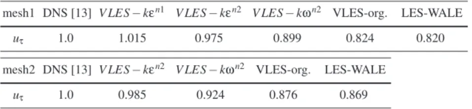
Table 1 Comparisons of friction velocity,uτ, between different models
mesh1 DNS [13] V LES−kεn1 V LES−kεn2 V LES−kωn2 VLES-org. LES-WALE
uτ 1.0 1.015 0.975 0.899 0.824 0.820
mesh2 DNS [13] V LES−kεn2 V LES−kωn2 VLES-org. LES-WALE
uτ 1.0 0.985 0.924 0.876 0.869
The computed friction velocities are compared in Table 1, where superscriptn1 refers to the use of the model constantn=4/3 andn2 refers to the use ofn=2 in Eq. 6,V LES−org. refers to the original Speziale’s model, andLES−WALE refers to the simulation using the LES WALE model [14]. It can be seen that the new VLES models clearly improve the results, compared with the original VLES model and LES model. The VLES-kεmodels predict quite good results compared with DNS.
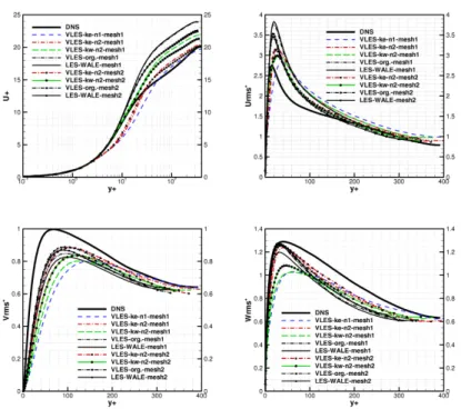
The mean streamwise velocity and RMS velocity profiles by different models are compared in Fig. 1. The first observation is that the new VLES model using the model constant ofn=2 predicts obviously better results than usingn=4/3. Therefore, in the following sections, the results shown are all obtained using the model constant ofn=2. The new VLES models based onk−ε andk−ω mod-els both improve the results compared with the original VLES model and with the LES WALE model. It should be noted that predictions made by the original VLES model and LES WALE are quite close in all velocity profiles on the same mesh. The new VLES model based on thek−εmodel gives slightly better results than the one based on thek−ωmodel, which can be observed in Table 1. It can also be seen that, with increasing mesh resolution, the predictions of the new VLES models are im-proved. However, the level of improvement is dependent on the underlaying RANS
Fig. 1 Comparisons of velocity and RMS velocity profiles for channel flow
turbulence model. Compared with VLES based on thek−εmodel, the VLES based on thek−ω is more sensitive to the mesh resolution. It seems that the new VLES based on thek−ε model is quite insensitive to the mesh resolution, which means that it can resolve quite reasonable results on a very coarse mesh. This feature can also be observed in the next case of flow past a square cylinder.
4 Results of turbulent flow past a square cylinder
The new VLES model is also applied for the flow past a square cylinder atRe= 22000 based on the cylinder edge lengthD. The square cylinder is aligned in the z(spanwise) direction and the inlet flow is set in thex(streamwise) direction. The computational domain is 20D×14D×4D. The lateral dimension 14Dis the same as in Lyn’s experiment [11], and the lateral boundaries are also subject to the wall boundary conditions to make the comparison with experiment more appropriate. Two different coarse meshes are used. The grid is clustered near the wall and the first node is located aroundy+=1.0. The first mesh is quite coarse with a resolution of 85×60×10 (about 0.048 million cells in total), and the second by refining the first mesh near the square cylinder (within 2.0D), results in a mesh containing about
0.144 million cells. This is still very coarse, compared with the LES studies in [17], which uses a mesh of about 0.485 million and 1.066 millon cells, and the DES stud-ies in [2], which uses a mesh with 8.467 million cells. The flow was simulated by both the new VLES models based on thek−εmodel andk−ωmodel respectively using the model constant of n=2. A non-dimensional time step,t∗=tU
inlet/D equal to 0.01, was used for all simulations.
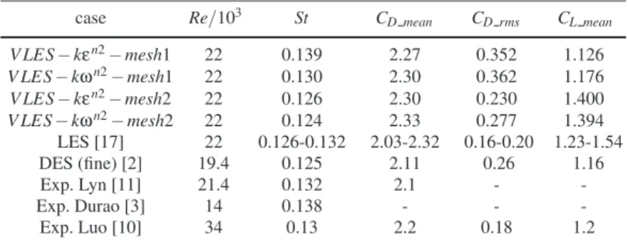
Table 2 Comparisons of global flow parameters between different models case Re/103 St C D mean CD rms CL mean V LES−kεn2−mesh1 22 0.139 2.27 0.352 1.126 V LES−kωn2−mesh1 22 0.130 2.30 0.362 1.176 V LES−kεn2−mesh2 22 0.126 2.30 0.230 1.400 V LES−kωn2−mesh2 22 0.124 2.33 0.277 1.394 LES [17] 22 0.126-0.132 2.03-2.32 0.16-0.20 1.23-1.54 DES (fine) [2] 19.4 0.125 2.11 0.26 1.16 Exp. Lyn [11] 21.4 0.132 2.1 - -Exp. Durao [3] 14 0.138 - - -Exp. Luo [10] 34 0.13 2.2 0.18 1.2
The global parameters of the flow fields are compared in Table 2 with some pre-vious studies. Although both meshes used are very coarse compared with prepre-vious numerical studies, all the global parameters predicted are acceptable. On the finer mesh, the results of RMS drag and lift coefficients are obviously improved. How-ever, the Strouhal number is slightly underpredicted and the mean drag coefficient overpredicted; this might resulted from the mesh used in the present study being very coarse. Previous DES studies [2] also found that the Strouhal number was un-derpredicted and the mean drag coefficient overpredicted when the mesh was not fine enough. The results also demonstrate that the new VLES model based on the k−εmodel is slightly better than the one based on thek−ω model.
The averaged and RMS velocities along the central line are compared in Fig. 2, and the averaged velocities at location x/D=1.0 are shown in Fig. 3. The new VLES predicts quite reasonable results on the quite coarse meshes compared with the LES results obtained in a dynamics Smagorinsky model in [17], and experi-mental data of Lyn et al. [11]. On the finer mesh, the VLES predicts better velocity distributions, especially for the RMS velocities. The results of the two VLES models are quite close based on thek−εmodel andk−ωmodel, except for the streamwise RMS velocity predictions. It can be seen that theUvelocities are quite higher than the experiments, but better than the LES results [17]. Previous simulations found that the velocity is quite hard to be accurately predicted unless the mesh is very fine. Considering that the finer mesh used for VLES simulations is much coarser than the DES study [2] (the total cell number used is about 1.7% of that in DES study), this might result in the overprediction ofU velocity. The underprediction ofWrmsmay also resulted from the coarse mesh as only 10 girds were placed in the spanwise di-rection. The performances of the VLES model on a finer mesh (around 1.0 million
Fig. 2 Comparisons of velocity and RMS velocity profiles along the central line including the LES results [17], DES results [2] and experiments [11]
cells) should be conducted later. However, these results still demonstrate that the new VLES model is quite efficient to resolve the flow field, and that comparative results can be obtained using much coarser computational meshes than in previous LES computations.
Fig. 3 Comparisons of streamwise and transverse velocity profiles at x/D=1.0 including DES results [2] and experiments [11]
5 Conclusions
A new Very Large Eddy Simulation (VLES) method was proposed in the present work that is based on Speziale’s VLES method. The new improved method can recover to a RANS simulation near the wall and also provide a proper LES mode between the limits of RANS and DNS. It was implemented in the standard k−
ε model and Wilcox’sk−ω model, and applied for turbulent channel flow and flow past a square cylinder. The results are compared with those of several previous studies. It is found that the new method is quite effective in resolving the large flow structures in both flow cases, and can give satisfactory predictions on a very coarse mesh compared with LES study, in both implementations based on thek−ε model and thek−ω model. It also seems that the new model is not sensitive to the mesh resolution, which implies that acceptable results can be obtained on very coarse meshes using the new model, which is an obvious advantage in complex engineering applications.
Appendix 1: VLES based on the standard
k
−
ε
model
The modeled transport equations forkandεare exactly the same as in the standard k−εmodel given by Dρk Dt =Pk−ρε+ ∂ ∂xj ·µ µ+µt σk ¶ ∂k ∂xj ¸ (10) Dρε Dt = ε k µ Cε1Pk−Cε2ρε ¶ + ∂ ∂xj ·µ µ+µt σε ¶ ∂ ε ∂xj ¸ (11) µt=FrρCµk2/ε (12)
The model constants are also exactly the same as in the standardk−εmodel. Func-tionFris shown in Eq. 6 and the length scales are given in Eq. 4.
Appendix 2: VLES based on Wilcox’s
k
−
ω
model
The modeled transport equations forkandωare exactly the same as in the Wilcox’s k−ωmodel, given by Dρk Dt =Pk−ρβ ∗ 0fβ∗kω+ ∂ ∂xj ·µ µ+µt σk ¶ ∂k ∂xj ¸ (13) Dρω Dt =α ω kPk−ρβ0fβω 2+ ∂ ∂xj ·µ µ+ µt σω ¶ ∂ ω ∂xj ¸ (14)
µt=Frρk/ω (15) The model constants are also exactly the same as in the Wilcox’s k−ω model (see [19] for details). FunctionFr is shown in Eq. 6. The length scales are calcu-lated in the framework of thek−ωmodel as
Lc=Cx(∆x∆y∆z) 1 3 L i=k 3 2/ε Lk=ν34/ε14 with ε=0.09kω (16)
References
1. Batten, P., Goldberg, U., Chakravarthy, S.: Interfacing statistical turbulence closures with large eddy simulation. AIAA J. 42, 485-492 (2004)
2. Barone, M.F., Roy, C.J.: Evaluation of Detached Eddy Simulation for turbulent wake appli-cations. AIAA J. 44, 3062-3071 (2006)
3. Durao, D.F.G., Heitor, M.V., Pereira, J.C.F.: Measurements of turbulent and periodic flows around a square cross section cylinder. Exp. Fluids 6, 298-304 (1988)
4. Fasel, H.F., Seidel, J., Wernz, S.: A methodology for simulations of complex turbulent flows. J. Fluids Eng. 124, 933-942 (2002)
5. Hsieh, K.J., Lien, F.S., Yee, E.: Towards a uniformed turbulence simulation approach for wall bounded flows. Flow Turbulence Combust 84, 193-218 (2010)
6. Israel, D.M.: A new approach for turbulent simulations in complex geometries. Ph.D. thesis, University of Arizona (2005)
7. Johansen, S.T., Wu, J.Y., Shyy W.: Filter-based unsteady RANS computations. Int. J. Heat Fluid Flow 25, 10-21 (2004)
8. Langhe, C. De, Merci, B., Dick, E.: Hybrid RANS/LES modelling with an approximate renor-malization group. I: model development. J. Turbulence 6, 1-18 (2005)
9. Liu, N.S., Shih, T.H.: Turbulence modeling for very large eddy simulation. AIAA J. 44, 687-697 (2006)
10. Luo, S.C., Yazdani, M.G., Chew, Y.T., et al.: Effects of incidence and afterbody shape on flow past bluff cylinders. J. Wind Eng. Ind. Aerodyn. 53, 375-399 (1994)
11. Lyn, D.A., Einav, S., Rodi, W., et al.: A laser-Doppler velocimetry study of ensemble-averaged characteristics of the turbulent near wake of a square cylinder. J. Fluid Mech. 304, 285-319 (1995)
12. Magnient, J.C., Sagaut, P., Deville, M.: A study of built-in filter for some eddy viscosity models in large eddy simulation, Phys. Fluids 13, 1440-1449 (2001)
13. Moser, R.D., Kim, J., Mansour N.N.: Direct numerical simulation of turbulent channel flow up toReτ=590. Phys. Fluids 11, 943-945 (1999)
14. Nicoud, F., Ducros, F.: Subgrid-scale stress modelling based on the square of the velocity gradient tensor. Flow Turbulence and Combustion 62, 183-200 (1999)
15. Peltier, L.J., Zajaczkowski, F.J.: Maintenance of the near-wall cycle of turbulence for hy-brid RANS/LES of fully-developed channel flow. In 3rd AFOSR International Conference on Direct Numerical Simulation and Large-Eddy Simulation. Kluwer Academic (2001) 16. Sagaut, P., Deck, S., Terracol, M.: Multiscale and multiresolution approaches in turbulence.
Imperial college press, London (2006)
17. Sohankar, A., Davidson, L.: Large Eddy Simulation of Flow Past a Square Cylinder: Com-parison of Different Subgrid Scale Models. J. Fluids Eng. 122, 39-47 (2000)
18. Speziale, C.G.: Turbulence modeling for time-dependent RANS and VLES: a review. AIAA J. 36, 173-184 (1998)
19. Wilcox, D.C.: Turbulence modeling for CFD. 2nd Ed., DCW Industries, Inc. (2004) 20. Zhang, H.L., Bachman, C.R., Fasel, H.F.: Application of a new methodology for simulations
![Fig. 2 Comparisons of velocity and RMS velocity profiles along the central line including the LES results [17], DES results [2] and experiments [11]](https://thumb-us.123doks.com/thumbv2/123dok_us/1877951.2774140/8.892.256.635.156.498/comparisons-velocity-velocity-profiles-central-including-results-experiments.webp)
