Tetrahedral mesh improvement via optimization of
the element condition number
Lori A. Freitag
1;∗;†and Patrick M. Knupp
2;‡1Mathematics and Computer Science Division;Argonne National Laboratory;Argonne;IL 60439;U.S.A. 2Parallel Computing Sciences Department;Sandia National Laboratories;M=S 0441;P.O. Box 5800;
Albuquerque;NM 87185-0441;U.S.A.
SUMMARY
We present a new shape measure for tetrahedral elements that is optimal in that it gives the distance of a tetrahedron from the set of inverted elements. This measure is constructed from the condition number of the linear transformation between a unit equilateral tetrahedron and any tetrahedron with positive volume. Using this shape measure, we formulate two optimization objective functions that are di!erentiated by their goal: the "rst seeks to improve the average quality of the tetrahedral mesh; the second aims to improve the worst-quality element in the mesh. We review the optimization techniques used with each objective function and present experimental results that demonstrate the e!ectiveness of the mesh improvement methods. We show that a combined optimization approach that uses both
objective functions obtains the best-quality meshes for several complex geometries. Copyright? 2001
John Wiley & Sons, Ltd.
KEY WORDS: mesh improvement; optimization-based mesh smoothing; mesh quality; element con-dition number
1. INTRODUCTION
Local mesh smoothing algorithms are commonly used for simplicial mesh improvement. These methods relocate a set of adjustable vertices, one at a time, to improve mesh quality in a neighbourhood of that vertex. The new grid point position is determined by considering a local submesh containing the adjustable, or free, vertex, v, and its incident vertices and elements.
∗Correspondence to: Lori A. Freitag, Mathematics and Computer Science Division, Argonne National Laboratory, 9700 South Cass Avenue, Argonne, IL 60439-4844, U.S.A.
†E-mail: [email protected] ‡E-mail: [email protected]
Contract=grant sponsor: O#ce of Advanced Scienti"c Computing Research, U.S. Department of Energy; contract=grant number: W-31-109-Eng-38
Contract=grant sponsor: Mathematics, Information and Computational Sciences Program (SC-31), U.S. Department of Energy; contract=grant number: DE-AC04-94AL85000
Overall improvement in the mesh is obtained by performing some number of sweeps over the set of adjustable vertices.
The most commonly used local mesh smoothing technique is Laplacian smoothing [1; 2] which moves the free vertex to the geometric centre of its incident vertices. Laplacian smooth-ing is computationally inexpensive but does not guarantee improvement in element quality. To address this problem, several optimization-based approaches to mesh smoothing have been developed in recent years [3–7]. In these techniques, the local submesh is evaluated according to some objective function based on a quality metric such as element angle or aspect ratio. Function and, possibly, gradient information are used to relocate the free vertex in such a way that the objective function is optimized.
Several optimization objective functions based on geometric criteria have been proposed for
a priori improvement of a simplicial mesh. For example, Bank proposed a ratio of triangle area to edge length squared for two-dimensional meshes [8], Shephard and Georges proposed a similar ratio of volume to face areas for tetrahedral meshes [3], Freitag et al. used angle-based measures for both two- and three-dimensional meshes [9;4], and Knupp has proposed a number of shape quality measures derived from simplicial element Jacobian matrices [7; 10]. Canann et al. proposed a distortion metric for both triangles and quadrilaterals that could be used with both valid and inverted elements [6]. In addition, a posteriori metrics have been proposed by Bank and Smith to improve "nite element meshes by optimizing solution error indicators [5].
In Section 2, we propose a new quality metric for the a priori improvement of tetrahe-dral meshes. The metric is based on the condition number of the linear transformation from an equilateral tetrahedron to an arbitrary tetrahedron. We show that the condition number metric is a tetrahedral shape measure according to the formal de"nition given in Dompierre
et al. [11], and that it is optimal in that it gives the distance of a tetrahedron to the set of inverted elements. We show that this previously overlooked metric is well-motivated, no more expensive to compute than other commonly used shape measures, and e!ective. In ad-dition, the condition number metric is notable because it is referenced to the ‘ideal’ element. This allows us to $exibly choose our ideal element shape and thereby reference element quality to an ideal anisotropic element as well as to an isotropic one. We have proved that the metric is equivalent (in the sense of Liu and Joe [12]) to the mean ratio metric [13; 14].
In Section 3, we formulate two optimization objective functions using the element condition number that are suitable for mesh improvement if the initial mesh is valid. The "rst objective function targets the improvement of average element quality and the second the improvement of the worst-element quality. In previous papers, we have independently proposed optimization techniques for mesh improvement as measured by average element quality [7] and mesh improvement as measured by extremal element quality [4], and we review these optimization techniques in Section 3.2. If the initial mesh is not valid, it may be preprocessed using an optimization-based mesh untangling approach that creates valid, although poor-quality, elements [15–17].
In Section 4, we present numerical results for each optimization approach on four tetrahedral meshes. We compare each technique to a baseline Laplacian smoother, and illustrate that in all test cases, a combined optimization approach produces the best-quality meshes. Finally, in Section 5, we o!er concluding remarks and directions for future research.
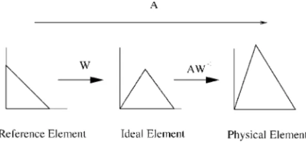
2. TETRAHEDRAL JACOBIAN MATRICES AND CONDITION NUMBERS To facilitate our discussion of the condition number quality metric, we "rst discuss the linear transformations associated with triangular and tetrahedral elements. Figure 1 illustrates the two-dimensional case. Let t be an arbitrary triangular element consisting of three vertices vn,
n= 0;1;2; with co-ordinates xn∈R3. De"ne the edge vectors
ek; n=xk−xn (1)
withk#=nandk= 0;1;2. Vertexvn has two attached edge vectors,en+1; n anden+2; n, where the
indices are taken modulo three. The columns of the Jacobian matrix, denoted A, consist of the edge vectors attached to a vertex. This linear transformation takes points in the reference triangle (a right-angled triangle) to points in the physical triangle, t. De"ne the matrix W
such that it transforms the reference triangle to an ideal, equilateral triangle. Then the matrix
S=AW−1 transforms the ideal triangle to the physical triangle. This linear transformation is
critical because it measures the deviation of the physical triangle from the ideal shape. A critical part of the theory to be presented are the matrix norms associated with these linear transformations, and we brie$y review that information now. LetI be the identity matrix and S an arbitrary matrix. The Frobenius norm of S is de"ned in terms of the trace:
|S|= [tr(STS)]1=2
The Frobenius norm is invariant to rotation matrices, that is, |SR|=|RS|=|S|, where R is a rotation matrix (RTR=I; det(R) = 1). If S is invertible, then S−1 exists, and one can de"ne
the adjoint matrix of S:
adj(S) = det(S)S−1
Similarly, matrices and linear transformations can be de"ned for tetrahedral elements, and we now construct a new tetrahedral shape measure based on the resulting norms and matrix condition number.
2.1. Tetrahedral Jacobian matrices
For the three-dimensional case, let T be an arbitrary tetrahedral element consisting of four vertices vn, n= 0–3 with co-ordinates xn∈R3. De"ne the edge vectors, ek; n, as in
Figure 1. The relationship between the linear transformations and the reference, ideal, and physical elements.
Equation (1) fork= 0–3 and note thaten; k=−ek; n. Each vertex vn of the tetrahedra has three
attached edge vectors, en+1; n, en+2; n, and en+3; n, where the indices are taken modulo four. In
this case, the Jacobian matrix at node n, denotedAn, consists of the columns of the triplet of
attached edge vectors, namely,
An= (−1)n(en+1; n en+2; n en+3; n)
Let !n be the determinant of An. A right-handed rule is assumed for the edge-ordering so that
!n¿0 for elements with positive volume. Let V(T) denote the volume of the tetrahedron. Theorem 1. The determinants of An are independent of n; that is !n=!0 for n= 1;2;3. Proof. Let M be the following constant matrix:
M= 1 1 1 −1 0 0 0 −1 0
The determinant of M equals 1. A direct calculation shows that
An=A0Mn
for n= 1–3. Taking the determinant of this expression gives !n=!0.
It is well-known that the volume of a tetrahedron is one-sixth of the Jacobian determinant [18], hence !0= 6V(T) and V(T)¿0 if and only if !0¿0. An element is said to be valid
if and only if !0¿0.
One can easily show that the following relationships hold for the Jacobian matrix:
|An|2=|en+1; n|2+|en+2; n|2+|en+3; n|2
and
|adj(An)|2=|en+1; n×en+2; n|2+|en+2; n×en+3; n|2+|en+3; n×en+1; n|2
which provide a geometric interpretation of the norms. The norm-squared of An is the sum of
the lengths-squared of the attached edge vectors and the norm-squared of the adjoint is the sum of the squares of the areas of the attached triangular faces.
Unlike the determinant !n, the norms of An and adj(An) are not independent of n because
not all of the lengths and areas of the tetrahedron a!ect the result for An. However, one can
create a weighted Jacobian matrix that is independent of n, as will be shown next.
De"ne an equilateral tetrahedron Te to have sides of length one and four vertices with the
co-ordinates (0;0;0), (1;0;0), (1=2;√3=2;0), and (1=2;√3=6;√2=√3). This tetrahedron serves as the ideal element. Let Wn be the Jacobian matrix at the nth vertex of Te. For example,
W0= 1 1=2 1=2 0 √3=2 √3=6 0 0 √2=√3 and w0= det(W0) =√2=2.
Theorem 2. Let T be any tetrahedron with Jacobian matrices An and Sn be the linear
transformation that takes Wn to An, then Sn=A0W0−1. That is,Sn is independent of n. Proof. By de"nition, SnWn=An. If n= 0, S0=A0W0−1. Theorem 1 applies to the matrices Wn of Te. Thus Wn=W0Mn for n= 1;2;3. Because An=A0Mn, we have the stated result.
In other words, there exists a unique linear transformation between the ideal tetrahedron Te
and the physical tetrahedron T. Thus, let us denote W0 by W and w0 by w.
Theorem 3. The norms |AnW−1| and |WA−n1| are independent of n. That is |AnW−1|=|A0
W−1
| and |WA−1
n |=|WA−01|.
Proof. The result for n= 0 is immediate. De"ne the matrix R=WMW−1, where M is
de"ned in the proof of Theorem 1. A direct calculation shows that Ris a rotation matrix with a positive determinant. Therefore, det(Rn) = 1 and (Rn)TRn=I for n= 1;2;3. Hence
|AnW−1|= |A0MnW−1|
= |A0W−1Rn|
= |A0W−1|
Similarly, the second result can be proved by observing that WA−1
n = (AnW−1)−1= (Rn)−1W
A−1
0 and showing that (Rn)−1 is a rotation matrix. 2.2. Tetrahedral condition numbers
LetT+ be any valid tetrahedron. ThenA−n1 exists, and one can compute the weightedcondition number of the matrix An
"w(An) =|AnW−1| |(AnW−1)−1|
Because (AnW−1)−1=WAn−1, Theorem 3 shows that"w(An) is independent of n which is not
true for the unweighted condition number "(An) =|An| |A−n1|. Now let A be any of the four
Jacobian matrices ofT+ and"w(A) =|AW−1| |WA−1|. Recall thatS=AW−1 is the linear
trans-formation taking the ideal element to the physical element; hence "w(A) =|S| |S−1|="(S).
That is, "(S) is the condition number of the linear transformation between the ideal and physical tetrahedron.
Theorem 4. Let S be derived from a tetrahedron with positive volume. Then 3="(S) is a tetrahedral shape measure.
Proof. We use the formal de"nition given in Dompierre et al. [11], to prove this assertion. That is, we show that 3="(S) is (1) continuous, (2) invariant to translations and rotations, (3) has values greater than zero and less than or equal to one, (4) has a value of one if and only if the element is ideal, and (5) has a value of zero for degenerate tetrahedra.
First, it is clear that |S| is a continuous function of the co-ordinates of T+, and likewise so
is |S−1
|. Therefore, "(S) is a continuous function of the co-ordinates of any tetrahedron with
positive volume.
Second, the Jacobian matrix is invariant to translations so"(S) is invariant to translations. Let ˜A=#RA with #¿0 and R a rotation matrix, corresponding to a uniform scaling and
rotation of the tetrahedron. Let ˜S= ˜AW−1. Since the Frobenius norm is invariant under
rota-tions, it is clear that "( ˜S) ="(S). Finally, "(S) is invariant to scaling because for any real number, $, the de"nition of condition number directly shows that "($S) ="(S).
Third, it is clear that 0¡3="(S). For any matrix, |S|2 is the sum of the squares of its
singular values %i. Thus
"2(S) ='
i; j(%i=%j)
2
This is a continuous function of three variables and its minimum may be found by computing the solution to @"2=@%
i= 0 with i= 1–3. The solution is %i=% where % is any positive
constant. Hence "(S)¿3. This shows that 0¡3="(S)61.
Fourth, suppose 3="(S) = 1. Then the singular values of S must be constant and S=%R. Then the Jacobian matrix associated with the tetrahedron must have the form A=%RW; in other words, 3="(S) attains its maximum value only if the tetrahedral element is a rotation and uniform scaling of the ideal tetrahedron. The converse is easy to show.
Fifth, the de"nition of a degenerate tetrahedral element given in Dompierre et al. [11], is somewhat vague. As noted, a tetrahedron with a small volume is not necessarily degenerate. This is re$ected in the properties of the condition number. For example, if A=$W, where 0¡$!1, then!=$3det(W) is small, but 3="
w($W) = 1. Thus a tetrahedron with small volume
does not necessarily make 3="(S) large. Dompierre et al. give an example of a degenerate tetrahedron, one whose volume goes to zero but at least some of the lengths do not. Suppose there exist constants b and c such that 0¡b6|S| and 0¡c6|adj(S)|. Then both |A| and
|adj(A)| are bounded below by a positive constant. Since
"(S) =|S| |adj(S)|=det(S)
the limit of 3="(S) as !→0 is zero. Hence, for the given example, the condition number satis"es the requirement that a shape measure go to zero for a degenerate element. In fact, the condition number provides a rigorous de"nition of a degenerate element. Let 0¡$!1 be given. Then T+ is degenerate if 3="(S)¡$.
The distinguishing feature between the condition number metric and the other weighted non-dimensional quality metrics given in Knupp [10] is given in the following well-known theorem [19] adapted to our current setting.
Theorem 5. 1="(S) is the greatest lower bound for the distance of S to the set of singular matrices.
Proof. Let S and X be 3×3 matrices with S non-singular and S+X singular. Write S+
X=S(I+S−1X). If|S−1X|¡1, then I+S−1X is non-singular. This would mean that S+X is
non-singular, so we must have |S−1X|¿1. But 16|S−1X|6|S−1| |X|; hence |X|=|S|¿1="(S).
Therefore
min{|X|=|S|: S+X singular}= 1="(S)
Since S is singular if and only if A is singular, we are guaranteed that minimization of
"(S) will increase the distance between A and the set of singular matrices.
2.3. The condition number of poor-quality tetrahedral elements
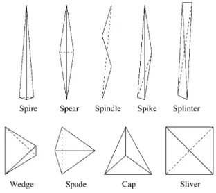
The second author reported numerical experiments which show that the common tetrahedral shape degeneracies can be detected by the condition number [10]. We now consider the taxonomy of poorly shaped tetrahedra given in Chenget al. [20], which is shown in Figure 2. The primary characteristic of these elements is that the four vertices are either nearly linear as shown in the top row or nearly planar as shown in the bottom row.
We now examine the behaviour of the condition number metric as the quality of each of the nine poorly shaped tetrahedra worsens. We report the value of the function "(S)=3 rather than 3="(S) so that "(S) = 1 for an ideal element and "(S)−→ ∞ as the element becomes increasingly distorted. We compare this metric to two commonly used quality metrics: minimum dihedral angle and element aspect ratio de"ned as
A&=
(1
6'6i=1L2i)3=2
8:47967V (2)
where Li is the length of each edge of the tetrahedron and V is the volume [13]. The aspect
ratio metric is also normalized so that A&= 1 corresponds to an ideal element and A&−→ ∞
as the element becomes increasingly distorted.
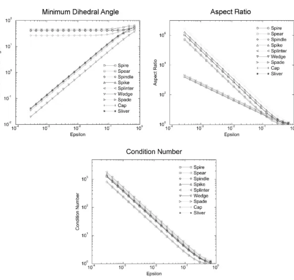
For each element type shown in Figure 2, we create a series of poor-quality tetrahedra and compute and plot the resulting metric values in the log–log graphs shown in Figure 3. We start with the ideal tetrahedral element and modify it so that the vertices are no more than a distance of $ from the centre line for the elements in the "rst row and are no taller than $for the element types in the second row. In Figure 3, we plot the values for each of the metrics as$
decreases. Ideally, the minimum dihedral angle should decrease as the tetrahedra become increasingly distorted. However, this metric is not a tetrahedral shape measure as de"ned
Figure 3. The minimum dihedral angle, aspect ratio, and condition number metrics as a function of tetrahedral element quality.
by Dompierreet al. [11] which is re$ected by the fact that it is unable to detect spear, spindle or spire elements. In contrast, both the aspect ratio and condition number metrics e!ectively detect all nine distorted element types. In addition, the dihedral angle metric is more expensive to compute than the other two because there are six values per tetrahedron rather than one. In particular, on a Sun Ultra 2 with 300 MHz processors, the dihedral angle metric required 1:73×10−4s to compute for each tetrahedron, whereas the aspect ratio and condition number
metrics required 3:80×10−5 and 6:58
×10−5s, respectively.
3. OPTIMIZATION-BASED SMOOTHING TECHNIQUES
Using the element condition number quality metric, we now derive two objective functions that are useful for optimization-based mesh improvement. We then brie$y describe the
associated optimization algorithms; more details can be found in the references mentioned below.
3.1. Optimization objective functions
To build objective functions for mesh improvement based on the condition number of the tetrahedron, consider a node in the interior of a valid tetrahedral mesh with M attached tetra-hedra. Let Am be a Jacobian matrix corresponding to the mth element and Sm=AmW−1. Let
"m="(Sm); m= 0;1; : : : ; M−1; be the weighted condition number of the mth attached
tetra-hedron normalized so that an equilateral tetratetra-hedron has a" value of one, andK= ("0; "1; : : : ;
"M−1). The vector p-norm of K can be used to construct a local objective function to
mini-mize the condition number
|K|p= (M−1 ' m=0" p m )1=p
The choice p= 2 gives the ‘2 norm of K
|K|2= (M−1 ' m=0 "2 m )1=2 (3) which can be used to minimize the average condition number, while p → ∞ gives the ‘∞
norm
|K|∞= maxm {"m}
which can be used to minimize the maximum condition number. For the results presented in Section 4, we reformulate the objective function as the equivalent maximization problem as follows:
Kmin= minm {−"m} (4)
Since the condition number is not de"ned for elements with negative volume, one must begin optimization with a valid mesh. To achieve this, the mesh is pre-processed with an untangling objective function based on the ‘∞ norm of the Jacobian determinant [15–17]. We note that some optimization techniques require the gradient of the condition number "(S) with respect to the free vertex position x. Let S=A W−1. One can apply the chain rule and
the formulas given in Knupp [10] to compactly write the gradient:
∇"= −@"@SW−Tu
with uT= [1;1;1]. An explicit calculation shows that @" @S= | S|2S det(S)2"(S)[|S|2I−STS]−"(S)S−T+|S−1|2 S "(S) 3.2. Optimization procedures
We now formulate the optimization problem associated with each of the objective functions given above. In each case, the characteristics of the objective function demand di!erent solu-tion techniques, and we brie$y describe the methods used.
3.2.1. Optimization of the ‘2 objective function. The formulation of the optimization
problem for the ‘2 objective function given in (3) is
min(M−'1
m=0"m(x)
2)
1=2
This objective function is smooth with continuous derivatives, and the problem can be solved with various techniques for unconstrained optimization.
We use a robust minimization algorithm that requires only objective function values. M
search directions are computed from the sum ofen+1; n for each of the attached tetrahedra. The
objective function is then evaluated at various distances along the scaled search directions, and the node is moved to the position that provides the greatest decrease in the value of the objective function. If no decrease is found, the node is not moved. See Knupp and Freitag [15] and Knupp [10] for more details.
3.2.2. Optimization of the ‘inf objective function. The optimization problem for the ‘inf
objective function given in (4) is formulated as max min
06m6M−1{−"m(x)}
where each "m is a non-linear, smooth, and continuously di!erentiable function of the free
vertex position. Let the maximum value of the functions evaluated at x be called the active value, and the set of functions that obtain that value, the active set, be denoted by S(x).
Since multiple elements can obtain the maximum value, the composite objective function has discontinuous partial derivatives where the active set changes from one set of functions to another set.
We solve this non-smooth optimization problem using an analogue of the steepest descent method for smooth functions. The search direction, s, at each step is the steepest descent direction derived from all possible convex linear combinations of the gradients in S(x). The
line search subproblem along s is solved by predicting the points at which the active set
S will change. These points are found by computing the intersection of the projection of a
current active function in the search direction with the linear approximation of each −"m(x)
given by the "rst-order Taylor series approximation. The distance to the nearest intersection point from the current location gives the initial step length, '. The initial step is accepted if the actual improvement achieved by moving v exceeds 90% of the estimated improvement or the subsequent step results in a smaller function improvement. Otherwise, ' is halved recursively until a step is accepted, or ' falls below some minimum step length tolerance. More detail on this optimization algorithm can be found in Freitaget al. [4] and Freitag [21].
4. NUMERICAL EXPERIMENTS
We now demonstrate the e!ectiveness of each of the optimization techniques in improving tetrahedral meshes compared with a baseline Laplacian smoother. We use four tetrahedral meshes generated by the CUBIT package [22] for duct, gear, hook, and foam geometries.
Figure 4. The four tetrahedral mesh test cases for duct, gear, hook and foam geometries. Table I. Initial quality of the four test cases.
Geom. N ND "avg "max A&avg A&max
Duct 4267 39 1.305 3.790 1.441 5.191
Gear 3116 25 1.423 3.448 1.622 4.782
Hook 4675 30 1.360 5.176 1.533 6.151
Foam 4847 47 1.392 4.362 1.579 8.197
These meshes are shown in Figure 4. In Table I, we give the number of elements in each mesh, N, and the initial mesh quality as measured by the following metrics:
1. The number of distorted elements in the mesh, ND, namely those with a normalized
con-dition number greater than 3.0.
2. The average normalized condition number for all of the elements in the mesh, "avg.
3. The maximum normalized condition number of any element in the mesh, "max.
4. The average and maximum tetrahedral aspect ratio given by Equation (2).
The overall quality of each initial mesh as measured by "avg andA&avg is quite good, but each
mesh contains a number of distorted elements.
Mesh improvement results are obtained by using the CUBIT and Opt-MS [23] software packages developed at Sandia National Laboratories and Argonne National Laboratory, re-spectively. An interface between these two packages has been developed, and we also report the results of a combined optimization approach that uses the two software packages in con-cert. We will measure the success of our smoothing techniques by their ability to eliminate distorted elements and to improve both the average and the maximum quality metric values. We attempt to improve each initial mesh described in Table I with six di!erent smoothing techniques:
1. Laplacian smoothing;
2. ‘Smart’ Laplacian smoothing, which accepts a Laplacian step only if the local submesh is improved as measured by "max;
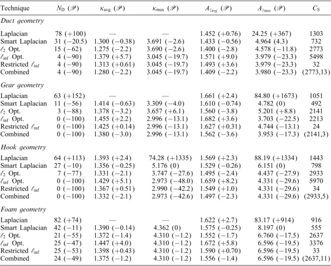
Table II. Mesh quality improvement results for the optimization-based smoothing techniques.
Technique ND (P) "avg (P) "max (P) A&avg (P) A&max (P) CS
Duct geometry Laplacian 78 (+100) — — 1.452 (+0:76) 24.25 (+367) 1303 Smart Laplacian 31 (−20:5) 1.300 (−0:38) 3.691 (−2:6) 1.433 (−0:56) 4.964 (4.3) 732 ‘2 Opt. 15 (−62) 1.275 (−2:2) 3.690 (−2:6) 1.400 (−2:8) 4.578 (−11:8) 2773 ‘inf Opt. 4 (−90) 1.379 (+5:7) 3.045 (−19:7) 1.571 (+9:0) 3.979 (−23:3) 5498 Restricted‘inf 4 (−90) 1.313 (+0:61) 3.045 (−19:7) 1.493 (+3:6) 3.979 (−23:3) 32 Combined 4 (−90) 1.280 (−2:2) 3.045 (−19:7) 1.409 (−2:2) 3.980 (−23:3) (2773,13) Gear geometry Laplacian 63 (+152) — — 1.661 (+2:4) 84.80 (+1673) 1051 Smart Laplacian 11 (−56) 1.414 (−0:63) 3.309 (−4:0) 1.610 (−0:74) 4.782 (0) 492 ‘2 Opt. 3 (−88) 1.378 (−3:2) 3.657 (+6:1) 1.560 (−3:8) 5.201 (+8:8) 2141 ‘inf Opt. 0 (−100) 1.455 (+2:2) 2.996 (−13:1) 1.682 (+3:6) 3.703 (−22:5) 2213 Restricted‘inf 0 (−100) 1.425 (+0:14) 2.996 (−13:1) 1.627 (+0:31) 4.744 (−13:1) 24 Combined 0 (−100) 1.380 (−3:0) 2.996 (−13:1) 1.562 (−3:6) 3.953 (−17:3) (2141,3) Hook geometry Laplacian 64 (+113) 1.393 (+2:4) 74.28 (+1335) 1.569 (+2:3) 88.19 (+1334) 1443 Smart Laplacian 27 (−10) 1.356 (−0:25) 5.176 (0) 1.529 (−0:26) 6.151 (0) 798 ‘2 Opt. 7 (−77) 1.331 (−2:1) 3.747 (−27:6) 1.495 (−2:4) 4.437 (−27:9) 2933 ‘inf Opt. 0 (−100) 1.429 (+5:1) 2.973 (−48:0) 1.659 (+8:2) 4.331 (−29:6) 5970 Restricted‘inf 0 (−100) 1.367 (+0:51) 2.990 (−42:2) 1.549 (+1:0) 4.331 (−29:6) 34 Combined 0 (−100) 1.332 (−2:1) 2.973 (−42:6) 1.497 (−2:3) 4.331 (−29:6) (2933,5) Foam geometry Laplacian 82 (+74) — — 1.622 (+2:7) 83.17 (+914) 916 Smart Laplacian 42 (−11) 1.390 (−0:14) 4.362 (0) 1.575 (−0:25) 8.197 (0) 555 ‘2 Opt. 21 (−55) 1.372 (−1:4) 4.310 (−1:2) 1.552 (−1:7) 6.760 (−17:5) 2637 ‘inf Opt. 25 (−47) 1.447 (+4:0) 4.310 (−1:2) 1.672 (+5:8) 6.596 (−19:5) 3376 Restricted‘inf 25 (−53) 1.398 (+0:43) 4.310 (−1:2) 1.590 (+0:70) 6.596 (−19:5) 33 Combined 24 (−49) 1.375 (−1:2) 4.310 (−1:2) 1.556 (−1:4) 6.596 (−19:5) (2637,11)
4. ‘inf smoothing as described in Section 3;
5. Restricted ‘inf smoothing that is applied only if "max¿3:0 in the local submesh; and
6. A combined optimization-based approach that uses ‘2 smoothing on each local submesh
followed by the restricted ‘inf approach.
In each case, we iterate over the interior nodes in the mesh until the change in all node point positions is smaller than some tolerance.
In Table II we report the results of each technique in terms of the number of distorted ele-ments remaining in the mesh after smoothing, the values of the quality metrics,qi="avg; "max; A&avg; A&max, as well as the percentage change from the initial value as computed by the formula:
Pi=qi"nalq−qiinitial iinitial
Owing to the way the metrics are normalized, a negative Pi value indicates an improvement
in mesh quality whereas a positive Pi value indicates a worsening of mesh quality. We also
report the number of nodes moved during the mesh smoothing process,CS, which corresponds
to the number of calls made to each smoother. For the combined approach, CS is reported as
the number of calls to the‘2 smoother, C1, plus the number of calls to the ‘inf smoother, C2,
and is denoted as (C1; C2).
In three of the four cases, Laplacian smoothing results in a mesh containing inverted el-ements. The CUBIT software de"nes the condition number of inverted elements to be 106,
which skews the "avg and"max values for those meshes; we do not report those results. In all
four cases, Laplacian smoothing worsens mesh quality by every measure reported: the number of distorted elements is approximately doubled, A&avg increases by more than 2%, and A&max is
signi"cantly worsened in all four cases. By design, the ‘smart’ Laplacian smoother improves the mesh in each case, but the improvement in the average element quality is less than 0.5% in all cases, and the improvement in the maximum quality values is zero in two of the four cases.
In contrast, the optimization-based smoothing approaches preserve mesh validity in all four test cases, and each approach signi"cantly improves the mesh by some measure of mesh quality. Both the ‘2 and ‘inf smoothers are able to eliminate a majority of the distorted
elements. The ‘inf smoother typically does better than ‘2 with respect to this metric, and in
two of the four cases eliminates all of the distorted elements from the mesh. As expected, the ‘2 smoother improves the average element quality in all four cases by as much 3.2%.
Although it is not designed to improve "max, this can happen serendipitously as is evidenced
in three of the four cases. In the gear geometry, however, "max worsens by about 6%. The
results for the ‘inf smoother are the inverse of the ‘2 results. The average element quality
is worsened in each case by as much as 5.7% in the duct geometry, but the "max and A&max
values are always signi"cantly improved. The restricted ‘inf smoother achieves nearly the
same improvement in "max and A&max as the ‘inf smoother without the corresponding decrease
in average element quality and at a signi"cantly smaller cost. The combined optimization approach achieves the best overall improvement in each of the four cases; all quality metrics are signi"cantly improved in all test cases, and its use is recommended.
In each case, the number of calls to the ‘2 smoother is roughly equal to the number of
vertices in the mesh. In contrast the ‘inf smoother is called more times, indicating more
grid point movement. This is supported by the fact that the average element quality changes approximately twice as much when the ‘inf smoother is called signi"cantly more times than
the ‘2 smoother. The restricted ‘inf smoother is called approximately once for each distorted
element in the mesh when used alone, and far fewer times when used in conjunction with the
‘2 smoother. Currently the ‘inf and ‘2 smoothers are about 10 and 100 times more expensive
than the smart Laplacian, respectively, and work to reduce computational cost is under way. 5. CONCLUSIONS
Our results indicate that the Laplacian smoothing can be detrimental to the quality of sim-plicial meshes on complex geometries, and we do not recommend its use. In contrast, the optimization approaches, particularly the combined ‘2 and ‘inf smoothing technique,
more commonly accepted aspect ratio shape measure was mirrored by the behaviour of the condition number shape measure, and that the condition number shape measure is theoretically optimal. In addition, the fact that the condition number metric can be referenced to any ideal element through the use of the weighting matrix makes it far more $exible than its geometric counterparts.
Strategically combining di!erent local mesh smoothing strategies is not a new idea; a number of researchers have combined Laplacian smoothing with their optimization-based ap-proaches to achieve good-quality meshes at a low computational cost [3;21]. However, this is the "rst instance we are aware of in which two optimization strategies have been combined to improve both the average element quality and the extremal element quality. Although our results showed that these improvements can be achieved for a small incremental cost to the
‘2 strategy, further work is needed to reduce the overall cost of the approach. Techniques
that combine Laplacian smoothing with the combined technique presented here are under consideration.
Finally, we note that the algorithms presented in this paper for smoothing and untangling are local techniques; a globally optimal solution is not guaranteed although empirical evidence suggests that the techniques work well in practice.
ACKNOWLEDGEMENTS
The work of the "rst author was supported by the Mathematical, Information, and Computational Sci-ences Division subprogram of the O#ce of Advanced Scienti"c Computing Research, U.S. Department of Energy, under Contract W-31-109-Eng-38. The work of the second author was supported by the Department of Energy’s Mathematics, Information and Computational Sciences Program (SC-31) and was performed at Sandia National Laboratories. Sandia is a multiprogram laboratory operated by Sandia Corporation, a Lockheed Martin Company, for the United States Department of Energy under Contract DE-ACO4-94AL85000.
REFERENCES
1. Field DA. Laplacian smoothing and Delaunay triangulations.Communications and Applied Numerical Methods
1988;4:709–712.
2. Lo SH. A new mesh generation scheme for arbitrary planar domains. International Journal for Numerical Methods in Engineering 1985;21:1403–1426.
3. Shephard M, Georges M. Automatic three-dimensional mesh generation by the "nite octree technique.
International Journal for Numerical Methods in Engineering 1991;32:709–749.
4. Freitag LA, Jones MT, Plassmann PE. An e#cient parallel algorithm for mesh smoothing. Proceedings of the Fourth International Meshing Roundtable, Sandia National Laboratories, 1995; 47–58.
5. Bank RE, Smith RK. Mesh smoothing using a posteriori error estimates.SIAM Journal on Numerical Analysis
1997;34(3):979–997.
6. Staten ML, Canann SA, Tristano JR. An approach to combined Laplacian and optimization-based smoothing for triangular, quadrilateral, and quad-dominant meshes. Proceedings of the Seventh International Meshing Roundtable, Sandia National Laboratories, 1998; 479– 494.
7. Knupp P. Achieving "nite element mesh quality via optimization of the Jacobian matrix norm and associated quantities. Part I—A framework for surface mesh optimization. International Journal for Numerical Methods in Engineering2000;48(3):401– 420.
8. Bank R.PLTMG:A Software Package for Solving Ellipitc Parital Di!erential Equations,Users’Guide7.0,
Frontiers in Applied Mathematics, vol. 15. SIAM: Philadelphia, PA, 1994.
9. Freitag L, Ollivier-Gooch C. A comparison of tetrahedral mesh improvement techniques. Proceedings of the Fifth International Meshing Roundtable, Sandia National Laboratories, 1996; 87–100.
10. Knupp P. Achieving "nite element mesh quality via optimization of the Jacobian matrix norm and associated quantities. Part II—A framework for volume mesh optimization. Technical Report SAND 99-0709J, Sandia National Laboratories, 1999.
11. Dompierre J, Labbe P, Guibault F, Camerero R. Proposal of benchmarks for 3D unstructured tetrahedral mesh optimization. Proceedings of the Seventh International Meshing RoundTable’98, 1998; 459– 478.
12. Liu A, Joe B. Relationship between tetrahedron quality measures.BIT1994;34:268–287.
13. Parthasarathy VN, Graichen CM, Hathaway AF. A comparison of tetrahedron quality measures.Finite Element Analysis and Design 1993;15:255–261.
14. Knupp P. Algebraic mesh quality metrics.Technical Report SAND 00-, Sandia National Laboratories, 2000. 15. Freitag L, Knupp P. Tetrahedral element shape optimization via the Jacobian determinant and condition number.
Proceedings of the Eighth International Meshing Roundtable, Sandia National Laboratories, 1999; 247–258. 16. Freitag, L, Plassmann P. Local optimization-based simplicial mesh untangling and improvement. Preprint
ANL=MCS-P749-0399, Mathematics and Computer Science Division, Argonne National Laboratory, Argonne, IL, August, 1999.
17. Knupp P. Non-simplicial mesh untangling.Technical Report SAND 00-, Sandia National Laboratories, 2000. 18. George PL, Borouchaki H.Delaunay Triangulation and Meshing. Hermes: Paris, 1998.
19. Demmel J.Applied Numerical Linear Algebra. SIAM: Philadelphia, PA, 1997.
20. Siu-Wing Cheng, Dey T, Edelsbrunner H, Facello M, Shang-Hua Teng. Sliver exudation.ACM Symposium on Compuational Geometry, 1999; 1–13.
21. Freitag, L. On combining Laplacian and optimization-based smoothing techniques. In Trends in Unstructured Mesh Generation, vol. AMD-vol. 220, Canann S, Saigal S (eds), New York: ASME Applied Mechanics Division, 1997; 37– 44.
22. Blacker TD, et al. CUBIT mesh generation environment. Technical Report SAND94-1100, Sandia National Laboratories, Albuquerque, NM, May 1994.
23. Freitag L. Users manual for Opt-MS: Local methods for simplicial mesh smoothing and untangling.Technical Report ANL=MCS-TM-239, Mathematics and Computer Science Division, Argonne National Laboratory, Argonne, IL, 1999.