Repository and Information Exchange
Electronic Theses and Dissertations2018
Statistical Algorithms and Bioinformatics Tools
Development for Computational Analysis of
High-throughput Transcriptomic Data
Adam McDermaid
South Dakota State University
Follow this and additional works at:https://openprairie.sdstate.edu/etd Part of theBiometry Commons, and theMathematics Commons
This Dissertation - Open Access is brought to you for free and open access by Open PRAIRIE: Open Public Research Access Institutional Repository and Information Exchange. It has been accepted for inclusion in Electronic Theses and Dissertations by an authorized administrator of Open PRAIRIE: Open Public Research Access Institutional Repository and Information Exchange. For more information, please [email protected]. Recommended Citation
McDermaid, Adam, "Statistical Algorithms and Bioinformatics Tools Development for Computational Analysis of High-throughput Transcriptomic Data" (2018).Electronic Theses and Dissertations. 2645.
STATISTICAL ALGORITHMS AND BIOINFORMATICS TOOLS DEVELOPMENT FOR COMPUTATIONAL ANALYSIS OF HIGH-THROUGHPUT
TRANSCRIPTOMIC DATA
BY
ADAM MCDERMAID
A dissertation submitted in partial fulfillment of the requirements for the
Doctor of Philosophy
Major in Computational Science & Statistics
South Dakota State University
ACKNOWLEDGEMENTS
I would like to thank my research advisors, Dr. Qin Ma and Dr. Anne Fennell, for their continued support throughout my advancement toward this degree. Both have been invaluable in helping me get to this point. Their support and guidance has allowed for me to comfortably convert from a student to competent researcher.
I would also like to thank the members of the Bioinformatics and Mathematical Biosciences Lab, especially Jinyu Yang, Juan Xie, Cankun Wang, Anjun Ma, and Yiran Zhang, as their assistance with numerous aspects throughout the last three years has been very much appreciated.
Finally, I would like to thank my family. Without their support, I would not be where I am today.
CONTENTS
ABSTRACT ... vii
CHAPTER 1: Introduction ... 1
1.1 Next-Generation Sequencing and RNA-Sequencing Analysis ... 1
1.2 Analysis Tools and Pipelines ... 2
1.3 IRIS Pipeline Framework ... 7
1.3.1 Preprocessing ... 7
1.3.2 Expression Estimation ... 8
1.3.3 End-Stage Analysis... 10
CHAPTER 2: Algorithms and Tools Development for RNA-Seq Data... 12
2.1 GeneQC: Gene Expression Estimation Quality Control ... 12
2.1.1 Mapping Uncertainty ... 12
2.1.2 Methods ... 17
2.1.3 Application on Real Data ... 28
2.1.4 Summary ... 31
2.2 ARM: Ambiguous Read Mapping Algorithm ... 33
2.2.1 Methods ... 34
2.2.2 Application on Real Data ... 38
2.3 IRIS-EDA: Integrated RNA-Seq Interpretation System for Gene Expression
Data Analysis ... 43
2.3.1 Gene Expression Data Analysis and Bottlenecks ... 43
2.3.2 Methods and Implementation ... 47
2.3.3 Summary ... 52
2.4 ViDGER: Visualization of Differential Gene Expression Results Using R ... 53
2.4.1 Interpreting Differential Gene Expression Results ... 53
2.4.2 Methods and Implementation ... 55
2.4.3 Summary ... 64
CHAPTER 3: Collaborative Efforts ... 64
3.1 Computational Tool Collaborations ... 64
3.1.1 Review of Motif Prediction Methods and DMINDA2.0 ... 64
3.1.2 RECTA: Regulon Identification Based on Comparative Genomics and Transcriptomics Analysis ... 67
3.1.3 Metagenomic and Metatranscriptomic Analysis & the Integrated Meta-Function Pipeline ... 71
3.2 Applications of Data Analysis in Collaborations ... 75
3.2.1 Human Cancer Cells ... 75
3.2.2 Malus domestica ... 78
REFERENCES ... 88 APPENDIX 1: Grant proposal to South Dakota Competitive Research Grant Program 119 APPENDIX 2: Curriculum vitae ... 126
ABSTRACT
STATISTICAL ALGORITHMS AND BIOINFORMATICS TOOLS DEVELOPMENT FOR COMPUTATIONAL ANALYSIS OF HIGH-THROUGHPUT
TRANSCRIPTOMIC DATA
ADAM MCDERMAID
2018
Next-Generation Sequencing technologies allow for a substantial increase in the amount of data available for various biological studies. In order to effectively and efficiently analyze this data, computational approaches combining mathematics, statistics, computer science, and biology are implemented. Even with the substantial efforts devoted to development of these approaches, numerous issues and pitfalls remain. One of these issues is mapping uncertainty, in which read alignment results are biased due to the inherent difficulties associated with accurately aligning RNA-Sequencing reads. GeneQC is an alignment quality control tool that provides insight into the severity of mapping uncertainty in each annotated gene from alignment results. GeneQC used feature extraction to identify three levels of information for each gene and implements elastic net regularization and mixture model fitting to provide insight in the severity of mapping uncertainty and the quality of read alignment. In combination with GeneQC, the Ambiguous Reads Mapping (ARM) algorithm works to re-align ambiguous reads through the integration of motif prediction from metabolic pathways to establish co-regulatory gene modules for re-alignment using a negative binomial distribution-based probabilistic approach. These two tools work in tandem to address the issue of mapping
uncertainty and provide more accurate read alignments, and thus more accurate expression estimates.
Also presented in this dissertation are two approaches to interpreting the expression estimates. The first is IRIS-EDA, an integrated shiny web server that combines numerous analyses to investigate gene expression data generated from RNA-Sequencing data. The second is ViDGER, an R/Bioconductor package that quickly generates high-quality visualizations of differential gene expression results to assist users in comprehensive interpretations of their differential gene expression results, which is a non-trivial task. These four presented tools cover a variety of aspects of modern RNA-Seq analyses and aim to address bottlenecks related to algorithmic and computational issues, as well as more efficient and effective implementation methods.
CHAPTER 1: Introduction
1.1 Next-Generation Sequencing and RNA-Sequencing Analysis
The advent of much improved biotechnology and the decreased associated costs have increased the amount of biological data. One of the most modern approaches is Next-Generation Sequencing (NGS) [1, 2], which has higher resolution, better accuracy, lower technical variation, and other advantages, compared with array-based counterparts [3-5]. NGS allows for a much faster-paced generation of larger volumes of biological information than ever before. The generated big data, which refers to the complex and large volumes of data collected from different sources, has changed the way research is conducted in biology [6, 7]. Although the availability of data has increased, utilizing and interpreting it requires new advances in interdisciplinary sciences, namely in
mathematics, statistics, and computer science. RNA-sequencing (RNA-Seq) and Chromatin Immunoprecipitation followed by sequencing (ChIP-Seq) have arisen and been used for the interpretation of transcriptional regulation. The RNA-Seq technology measures the abundance of RNA transcripts in samples or individual cells, giving rise to
the genome-scale transcriptomic (also termed as gene expression) data [8].
ChIP-Seq technologies provide massive amounts of information related to protein-DNA interactions and have been applied successfully to many genome-wide analyses, including transcription factor binding, polymerase binding, and histone modification markers [9, 10]. This type of data is especially useful for determination of transcriptional regulatory signals (TRSs), such as transcription factors (TFs), miRNAs, lncRNAs, and epigenomic regulators. TFs are known to play an important role in
controlling gene expression by binding to specific DNA sequences, with their TF binding
sites (TFBSs) are referred to as cis-regulatory motifs (motifs for short).
RNA-Seq is a revolutionary technology for gene expression profiling [11, 12] and promises to provide a comprehensive picture of the transcriptome for a biological process [11]. It aims to extract usable information from the mature mRNA within a biological
source and generates a huge number of short segments (reads, 100-250 bps), which
enable the discrete quantification of all genes expressed in a cell [11, 13]. Currently, researchers can analyze a large sample of cells from a single organism in the form of bulk RNA-Seq data or can discover individual cells from complex organisms one at a time through single-cell RNA-Sequencing (scRNA-Seq), which uses optimized NGS
technologies and acquires the transcriptomic information from individual cells to provide a better understanding of cell functions at genetic and cellular levels [14]. These
biotechnologies have generated large-scale transcriptomic data and genome-scale gene expression data in the public domain, and their tremendous values have been confirmed in many research areas such as elucidation of cell-type-specific regulatory networks [15, 16] and cancer & complex diseases studies [17-19]. Although numerous algorithms and tools have been developed for transcriptomic data analysis, both in the public [20-46] and private sectors [47-54], the reality is that some of the most widely-used methods suffer from particular issues (e.g., cannot provide accurate gene expression estimates [55, 56]) and construction of applicable combinations of these tools is an ongoing challenge.
1.2 Analysis Tools and Pipelines
RNA-Seq analyses begins with data collection from biological samples. During this process, mature mRNA is extracted from single or multiple cells of a particular
sample with specific characteristics. This mRNA is reverse transcribed into cDNA, which is then broken apart into small segments, referred to as reads. These short reads are generally 80 to 250 base pairs (bps) in length. There are also emerging third-generation sequencing technologies that generate reads in the several mbp lengths; although these approaches can suffer from high error rates during sequencing, limiting their current application power [1, 57, 58]. The set of these reads—generally in the range of millions of reads—is referred to as the library of raw reads for analysis in an RNA-Seq experiment.
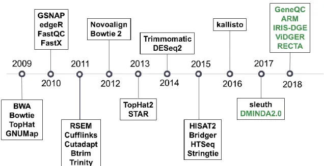
Analyzing raw reads requires numerous steps, and thus requires numerous tools (Figure 1). To effectively use these tools in combination, a pipeline is generally
established with the user’s tools of choice. Initially, a read level quality control is conducted on the raw reads. FastQC [20] is almost universally used for this purpose and provides information related to sequencing depth, reads duplication rates, GC bias, coverage uniformity, among other features. Any serious issues detected in this initial process are then corrected through read trimming. This process trims the end segments off the raw reads, which tend to have remnants of the sequencing process. For this purpose, numerous tools have been developed and are widely implemented in
application, including Btrim [59], the Fastx toolkit [60], Trimmomatic [61], and Cutadapt [62]. To verify successful data trimming, read-level quality control can be used again.
Figure 1: High-performing and widely used RNA-Seq tools developed since 2009. Green lettering indicates tools that are covered in this dissertation, between Chapters 2 & 3.
After verifying the integrity of the raw RNA-Seq data, multiple steps are conducted to quantify the read counts for each gene, which provides insight into the expression level for each gene of each sample. If a reference genome is available for the given species, reference-based read alignment (also referred to as read mapping) of raw or trimmed reads determines where along the genome each read came from. While time consuming and computationally demanding, this step is one of the most important processes used in most RNA-Seq analyses. Due to the importance, numerous tools have been developed for this purpose, including TopHat [35], BWA [63], Bowtie [64, 65], and HISAT [40], among many others [29, 31-33, 37, 42, 44].
Read alignment results still require further analysis to quantify the number of reads estimated at each gene. Two distinct pathways can be pursued at this point. The first is direct quantification of gene expression through read counts. Using a species-specific annotation file, quantification tools take the read alignment results and determine
to which gene each read is aligned. Based on this information, a discrete count of the expression for each gene is generated. Again, there are many tools that can perform this purpose, with HTSeq [45] being one common and efficient method. Alternatively, the second path requires another extensive computational approach in what is referred to as assembly. Assembly tools, such as StringTie [38, 39] and Cufflinks [34], take the aligned reads and assemble transcripts from these segments. The abundance of these transcripts is then quantified, providing an expression estimate. The assembly step is increasingly useful to determine novel transcripts that have not been annotated in a particular species and for addressing the issues presented by alternative splicing. Both of these two approaches result in an estimate of the expression level for each gene.
Having a reference genome for RNA-Seq analysis is not always possible. Some species being analyzed may not have a reference genome sequences at the time of
analysis, requiring a different approach. De novo assembly is a process that can develops
a transcriptome through alignment of the reads themselves. In this process, the reads are taken and assembled together based on overlapping sequences of various lengths. A De
Bruijn graph approach is most commonly used for this purpose by most de novo
assembly tools, such as Trinity [66, 67] and Bridger [43]. The assembly can then be used to functionally annotate the regions within the transcriptome.
Using the expression estimations generated through the reference-based approaches, numerous additional analyses can be performed. One such analysis is differential gene expression analysis, in which gene expression levels are compared between samples of particular conditions. This approach can provide insight into the genetic differences that are affecting or correlated with observed phenotypic differences.
Functional annotation is a process using expression estimates that look for highly expressed functional groups of genes within particular samples. This process can also include comparison of functional group expressions across two or more conditions. Traditional clustering approaches, such as k-means [68] or hierarchical clustering [69], can also be directly applied to expression estimates through grouping of similarly expressed samples. This method can provide insight into which samples or conditions have expression-wide similarities. Biclustering is a two-dimensional clustering approach [70] that, when applied to expression matrices, groups samples together based on subsets of the expression estimates [71]. Since it can be expected that genetic similarities can be exhibited in only a small portion of the expression estimates, this approach captures these similarities and groups sample together, as opposed to requiring high similarity
throughout all expression estimates. Particularly, biclustering has the special application power in scRNA-Seq analyses [72, 73]. In addition to these defined approaches, there are virtually endless other analyses that can be performed using the expression estimates, including a wide range of network analyses and other modeling approaches.
Although substantial efforts have been made to accurately and efficiently quantify genetic expression levels, the performance of these tools is not always adequate. Many of the tools have been shown to underperform on real or synthetic RNA-Seq datasets [55, 56]. TopHat [34, 35], one of the most widely used read alignment tools, has even been demonstrated as one of the poorest performing, having less than 20% of reads correctly aligned in some cases [55]. Even combinations of tools that have excellent individual performance can result in suboptimal or even poor performance levels [56]. Hence,
further investigation into optimized approaches for high-throughput data analysis is required.
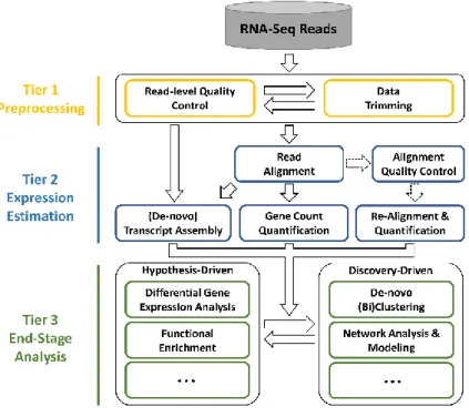
1.3 IRIS Pipeline Framework
All tools related to RNA-Seq analysis fit into a three-tier framework based both on the placement they fit into and analysis function, referred to as the Integrated RNA-Seq data analysis and Interpretation System (IRIS). This framework consists of tiers representing preprocessing, expression estimation, and end-stage analysis (Figure 2).
Figure 2: The IRIS Pipeline. The IRIS pipeline consists of three tiers
designed to analyze and interpret RNA-Seq data. Tier 1 involves preprocessing, Tier 2 determines expression estimates, and Tier 3
provides end-stage analyses 1.3.1 Preprocessing
Preprocessing consists of tool related to quality control for the raw RNA-Seq reads. There are two analyses in this tier, the first being read-level quality control. This process involves investigation of the raw reads to determine if any abnormalities exist,
including detection of primers used to sequence the raw reads. FastQC [20] is almost universally used for this process, and provides statistics related to per base sequence quality, per sequence quality scores, per base sequence content, per base and per
sequence GC content, Kmer content, among other important measures. Users can make decisions about the quality of their raw reads based on the provided information and determine if they need additional measures, such as data trimming. Data trimming involves modification of the raw reads to remove poor sequences and sequence segments, including primers remaining on the ends of reads from previous steps. A wide variety of tools can be utilized for this purpose [28, 60-62]. The results of Tier 1 used for further analysis are either the raw reads—in the case that there are no serious issues found during quality control—or trimmed reads generated using one of the read trimming tools.
1.3.2 Expression Estimation
Using the raw or trimmed reads from Tier 1, Tier 2 contains tools that convert the reads to expression estimates, generally in conjunction with additional genomic
information in the form of a reference genome and annotation. This tier is the core of RNA-Seq data analysis and can proceed through multiple unique paths. Which path is pursued is determined by which data is being analyzed, availability of a reference genome, and investigative purposes. If a reference genome is not available, the
reference-based approaches are not applicable. In these cases, De novo assembly is used
and is commonly combined with annotation of sequences to determine which genes are present and to some degree a measure of the expression level.
The alternative pathway, one in which a reference genome is available, involves alignment of reads against the reference genome. This process is generally time
consuming and computationally demanding. Numerous approaches have been developed for this purpose [29, 31-33, 35, 37, 40, 42, 44, 63-65], with key emphasis on reducing the time and computational requirements.
After read alignment, there are another level of pathways that can be followed. A straightforward quantification of read counts based on the read alignment can generate a discrete estimation of the expression level for each annotated gene. Alternatively,
reference-based transcript assembly can be used to generate transcripts for quantification. A third approach that is much more recent has to do with mapping uncertainty, which results when a read can be aligned to multiple locations. To address this issue, new approaches have been developed for quality control and read re-alignment.
From these pathways, users generally determine an estimation of the genetic expression levels from their samples. Depending on the tools and methods used, the measurement used for expression level can vary. Some methods generate read counts, with a discrete count of the number of reads aligned to each location is provided. Others provide normalized measures based on the gene length or raw read library size. Four commonly used normalized measures are Reads Per Kilobase per Million (RPKM), Fragments Per Kilobase per Million (FPKM), Transcripts Per kilobase per Million (TPM), and Counts Per Million mapped reads (CPM). RPKM and FPKM are calculated similarly, with the former being used for single-end reads and the latter for paired-end
reads. The calculations for normalized counts for a given gene i are given below, with 𝐿
representing library size (i.e. number of reads analyzed), 𝑔𝑖 representing the length of
𝐹𝑃𝐾𝑀𝑖 = 𝑅𝑃𝐾𝑀𝑖 = 𝑐𝑖 𝐿/106÷ 𝑔𝑖 = 𝑐 𝐿 ∗ 𝑔𝑖 ∗ 10 6 𝑇𝑃𝑀𝑖 = 𝑐𝑖 𝑔𝑖 ∑ 𝑐𝑗 𝑔𝑗 𝑗 ÷ ( 𝐿 106) = 106 ∗𝑔𝑐𝑖 𝑖 𝐿 ∗ ∑ 𝑔𝑐𝑗 𝑗 𝑗 𝐶𝑃𝑀𝑖 = 𝑐𝑖 𝐿 106 =𝑐𝑖 𝐿 ∗ 10 6
Frequently, all of these measures are represented in using a logarithm base-10 transformation, since measures can vary greatly.
1.3.3 End-Stage Analysis
From the expression estimates generated in Tier 2, a wide range of analyses can be performed to make biologically meaningful interpretations from the data. Tier 3 contains analysis tools related to this conversion of expression estimates to practical interpretations and is divided into two categories: Hypothesis-driven interpretations and Discovery-driven interpretations. Hypothesis-driven analyses are generally conducted following previously established hypotheses and concepts. Included in this category are differential gene expression analysis and functional enrichment analysis, among many other processes. Differential gene expression analysis is one of the most common analyses used in the analysis of RNA-Seq data and uses statistical techniques to find meaningful differences in expression levels between comparable conditions. This process uses raw or normalized read counts from replicates of the same condition to identify which genes are statistically differentially expressed between two or more conditions. One common use of this method is to determine which genes have differing expression levels for two different strains of the same species that exhibit important
phenotypic differences. This investigation can lead to further understanding of specific relationships between genotype and phenotype.
Discovery-driven analyses follow a more purely exploratory approach, one aimed at discovering interesting features from the data, as opposed to being directed at a
specific hypothesis. Included in this category are clustering and biclustering methods and a wide range of network analyses. Rapidly growing in the analysis of RNA-Seq data is the use of biclustering approaches [70, 74], which isolate similarities between conditions and samples using only a subset of the gene expression estimates. It has been widely shown that most plant and animal life on earth has high genetic similarity due to
commonalities in cellular structure and function [75], meaning the genetic differences in a single species, regardless of their phenotypic differences, will be relatively mild. Because of this, clustering samples based on total genetic expression may miss significant expression patterns. While traditional clustering looks for conditions or samples that have similar expression levels across all genes, biclustering can identify similarities that exist in only a fraction of the total genetic expression profile.
While the analyses included in Tier 3 generally represent the end-stage analyses, there are many times overlaps and feedback loops within this stage. For instance, cell type classification of single-cell RNA-Seq data may involve initial clustering or
biclustering combined with additional graph modeling to identify which cells belong to the same cell type. This means that an end-stage analysis may not necessarily be the final analysis step in an RNA-Seq pipeline, since end-stage analyses can be layered for a specific purpose. However, most experiments using RNA-Seq data will have a well-defined design relying on direct results from Tier 3.
CHAPTER 2: Algorithms and Tools Development for RNA-Seq Data
While there have been great amounts of effort done towards designing optimized RNA-Seq analysis tools, this area of research is by no means complete. The nature of dealing with big data analysis always means a never-ending striving for increased efficiency, both in terms of the time and computational requirements. Additionally, dealing with data and results that frequently consist of tens-of-thousands of measures of statistical significance and an equal number of measures of magnitude leads to challenges with interpreting results on a global scale. Even more challenging are prominent issues within analysis pipelines that arise from biological complexities, such as the
determination of the correct alignment location for a single RNA-Seq read. All of these challenges combined promote the need for continued development of analysis tools for RNA-Seq data. In this chapter, I present four tools develop to address specific pitfalls within RNA-Seq pipelines.
2.1 GeneQC: Gene Expression Estimation Quality Control
2.1.1 Mapping Uncertainty
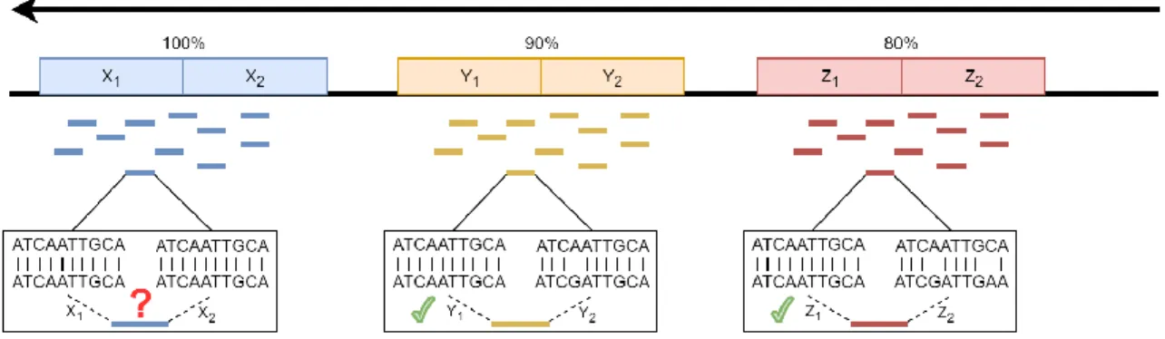
Even though numerous methods have been developed to facilitate read alignment, some critical issues persist. The nature of DNA—long strands of millions of base-pairs created by a reordering of the four nucleotides—makes it inevitable that some similarities and duplications will occur throughout the genome. This can lead to ambiguity during read mapping (Figure 3), with specific reads being aligned to multiple locations across the reference genome with the same alignment scores [7, 27, 55, 76-78]. When this issue
Figure 3: Mapping Uncertainty. Mapping uncertainty occurs when a single read can be mapped to two or more locations along the reference genome with equal or nearly equal confidence.
This mapping uncertainty problem can be observed in any genomic region, including, exons and transcripts. For conciseness, these genomic regions are simply referred to as "genes." This issue has been observed in many diploid species, including human and other mammals and Arabidopsis [79-83], as well as many multiploid species
[84]. In some species, such as Glycinemax, up to 75% of the genes have the duplicated
partners in its genome. For species with high levels of uncertainty, especially angiosperms, mapping uncertainty can have serious implications on gene expression levels and can be extremely hard to remediate due to the genes’ and chromosomes’ duplicative nature [41].
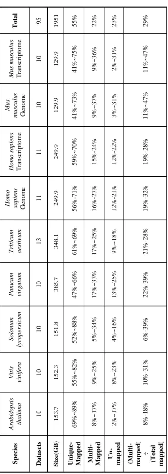
To more fully investigate the issue of mapping uncertainty, 95 datasets totaling almost two terabytes of RNA-Seq data was analyzed from seven plant and animal species with respect to their alignment statistics, including the percentages of uniquely-mapped reads, ambiguously-mapped reads, and non-mapped reads (Table 1). This analysis was done using HISAT2 [40] for read alignment, which automatically generates alignment statistics.
Both paired- and single-end reads were collected from NCBI [85], URGI (https://urgi.versailles.inra.fr/), and JGI [86] for seven plant and animal species. These
species include Arabidopsis thaliana, Vitis vinifera, Solanum lycopersicum, Panicum
virgatum, Triticum aestivum, Homo sapiens, and Mus musculus. The 83 paired-end datasets and 12 single-end datasets average 20.6 GB, with an average overall alignment rate of 81.87%. Each dataset was aligned using HISAT2 [40] against the appropriate reference genome.
Alignment statistics were collected or calculated from the HISAT2 output file, as shown in Table 1. It was determined that an average of 22% of all reads were
ambiguously aligned in each of the seven distinct plant and animal species. In four datasets, over 35% of the reads were ambiguously aligned, and over two-thirds of the
analyzed datasets having at least 18% of the reads multi-mapped. Panicum virgatum
exhibited the highest overall proportions—ranging from 17% to 33%—of multi-mapped
reads over all analyzed datasets, while Arabidopsis thaliana displayed the lowest
proportion, ranging from 8% to 17%. The other analyzed species had similar percentages of multi-mapped reads.
If researchers continue processing RNA-Seq data with such high levels of mapping uncertainty, all downstream analyses will have skewed and biased results. Just as raw reads require quality control [20] so do gene expression estimates based on mapping results. Even with tools that are specifically designed to address mapping uncertainty,
such as MMR [87], the quality of the derived gene expression estimates based on
datasets. Without some quality control for gene expression estimation, researchers could potentially be using unreliable data, and blindly doing so.
Table 1 : A li g nm ent Sta ti st ics . Sev en s p ec ies , fi v e p la nt and tw o a ni m al , w er e a li g ned us ing H ISA T 2. A li g nm ent st at is ti cs w er e col lec ted and p res ent ed bas ed on the per ce n t of r eads f al li ng int o ea ch ca teg or iz at ion . A lso inc luded ar e num ber of dat ase ts a n d ov er al l d at a si ze f or ea ch spe ci es . S p ec ies Ara b id o p sis th a li a n a Vitis vin ifer a S o la n u m ly co p er sic u m Pa n ic u m virg a tu m T riti cu m a es tivum Ho mo sa p ien s G en o m e Ho mo sa p ien s T ra n sc rip to m e M u s mu sc u lu s G en o m e M u s mu sc u lu s T ra n sc rip to m e To ta l Da ta se ts 10 10 10 10 13 11 11 10 10 95 S ize (G B ) 1 5 3 .7 1 5 2 .3 1 5 1 .8 3 8 5 .7 3 4 8 .1 2 4 9 .9 2 4 9 .9 1 2 9 .9 1 2 9 .9 1 9 5 1 Un iq u e-M a p p e d 6 9 % ~ 8 9 % 5 5 % ~ 8 2 % 5 2 % ~ 8 8 % 4 7 % ~ 6 6 % 6 1 % ~ 6 9 % 56% -7 1 % 5 9 % ~ 7 0 % 4 1 % ~ 7 3 % 4 1 % ~ 7 5 % 55% M u lti - M a p p e d 8 % ~ 1 7 % 9 % ~ 2 5 % 5 % ~ 3 4 % 1 7 % ~ 3 3 % 1 7 % ~2 5% 16% -2 7 % 15% -2 4 % 9 % ~ 3 7 % 9 % ~ 3 6 % 22% Un -m a p p ed 2 % ~ 1 7 % 8 % ~ 2 3 % 4 % ~ 1 6 % 1 3 % ~ 2 5 % 9 %~ 1 8% 12% -2 1 % 12% -2 2 % 3 % ~ 3 1 % 2 % ~ 3 1 % 23% (M u lti -m a p p ed ) ÷ (To ta l m a p p ed ) 8% -18% 10% -3 1 % 6% -39% 22% -3 9 % 21% -2 8 % 19% -3 2 % 19% -2 8 % 1 1 % ~ 4 7 % 1 1 % ~ 4 7 % 29%
2.1.2 Methods
To address this issue, I present GeneQC [88] based on novel applications of regularized regression and mixture model fitting approaches to quantify the mapping uncertainty issue (Figure 4). This tool can determine the genes having reliable expression estimates and those requiring further analysis, along with a statistical evaluation of the mapping uncertainty level. GeneQC develops a novel score, referred to as D-score, to represent the level of mapping uncertainty for each annotated gene and groups genes into several categorizations with different reliability levels, through integration and modeling of three genomic and transcriptomic features. Specifically, (i) sequence similarity
between a particular gene and other genes is collected to give an insight into the genomic characteristics contributing to the mapping uncertainty problem; (ii) the proportion of shared multi-mapped reads between gene pairs provides information regarding the transcriptomic influences of mapping uncertainty within each dataset; and (iii) the degree of each gene, representing the number of significant gene pair interactions resulting from calculating (i) and/or (ii).
Figure 4: GeneQC Workflow. (A) The MMR percentages for the 95 datasets across seven species. More detailed information is showcased in Table 1; (B) GeneQC takes a read alignment,
reference genome, and annotation file as inputs; (C) The first step of GeneQC is to extract features related to mapping uncertainty for each annotated gene; (D) Using the extracted features,
elastic-net regularization is used to calculate the D-score, which represents the mapping uncertainty for each gene; (E) A series of Mixture Normal and Mixture Gamma distributions are fit to the D-scores; and (F) The mixture models are used to categorize the D-scores into different levels of mapping uncertainty along with a statistical alternative likelihood value for each gene.
GeneQC is designed to fit into computational pipelines for RNA-Seq data
immediately following read alignment, acting as a supplement to most current pipelines. GeneQC is composed of two distinct processes: feature extraction and statistical
modeling. GeneQC takes as inputs three pieces of information that are easily found in most RNA-Seq analysis pipelines: (1) the read mapping result SAM file; (2) the fasta reference genome corresponding to the to-be-analyzed species; and (3) the species-specific annotation general feature format (gff/gtf/gff3) file (Figure 4B).
From input information, GeneQC first performs feature extraction, in which the three characteristics are calculated for each annotated gene (Figure 4C). The first
extracted feature (𝐷1) is derived from genomic level information and involves the similarity between two genes (Figure 5A). For each gene, this is calculated as the maximum of the sequence similarity multiplied by the match length, where the match length is the longest continuous string of matching base pairs. More specifically,
𝐷1 = max
𝑦 {𝑠𝑠𝑖,𝑦∗ 𝑙𝑖,𝑦}
where 𝑠𝑠𝑖,𝑦 is the base pair sequence similarity of gene 𝑖 and gene 𝑦 and 𝑙𝑖,𝑦 is the match
length of these two genes. Additionally, to minimize negligible interactions, some
default criteria are required for determination of 𝐷1: (1) 𝑠𝑠𝑖,𝑦∗ 𝑙𝑖,𝑦 > 100; (2)
𝑚𝑖𝑠𝑚𝑎𝑡𝑐ℎ 𝑐𝑜𝑢𝑛𝑡 < 5; (3) max{𝑔𝑎𝑝} < 5; and (4) 𝑒 − 𝑣𝑎𝑙𝑢𝑒 < 10−6 as determined in using BLAST [89].
Figure 5: (A) Genes with significant similarity are displayed, with 𝐷1 being the maximum value
of 𝑠𝑠𝑖,𝑦∗ 𝑙𝑖,𝑦. In this situation, genes 𝑦2, 𝑦3, & 𝑦4 all have the same 𝑠𝑠𝑖 value, but gene 𝑦3 has a
longer consecutive string of matching base pairs (𝑙𝑖) than the other values, making it the more
similar genomic location. (B) Graphical representation of the sets of reads aligned to each gene. 𝐷2 is the largest overlapping proportion of shared ambiguous or multi-mapped reads between the
to both locations. (C) This graph displays the significant interactions of gene 𝑖 with other genomic locations. Each node represents a genomic location, with the red edges representing
sequence similarity scores and black edges representing multi-mapping proportions. In this situation, 𝐷1= 310, 𝐷2= 0.24, and 𝐷3= 𝑙𝑜𝑔10(3 + 1) = 0.602.
The second feature (𝐷2) comes from transcriptomic level information and
represents the proportion of shared MMRs (Figure 5B). This value is calculated as the maximum proportion of shared MMRs between the gene of interest and another gene. In other words,
𝐷2 =|𝐺𝑖 ∩ 𝑋| |𝐺𝑖|
where 𝐺𝑖 = {𝑎𝑙𝑙 𝑟𝑒𝑎𝑑𝑠 𝑎𝑙𝑖𝑔𝑛𝑒𝑑 𝑡𝑜 𝑔𝑒𝑛𝑒 𝑖} and 𝑋 = argmax
𝑌
|𝐺𝑖 ∩ 𝑌|.
The third feature (𝐷3) is a network factor that represents the number of alternate
gene locations with significant interactions with the gene of interest based on the previous two parameters (Figure 5C) and is calculated as
𝐷3 = log10(|𝑆 ∪ 𝑀| + 1)
where 𝑆 = {𝑔𝑒𝑛𝑜𝑚𝑖𝑐 𝑙𝑜𝑐𝑎𝑡𝑖𝑜𝑛𝑠 𝑤𝑖𝑡ℎ 𝐷1 > 0} and 𝑀 =
{𝑔𝑒𝑛𝑜𝑚𝑖𝑐 𝑙𝑜𝑐𝑎𝑡𝑖𝑜𝑛𝑠 𝑤𝑖𝑡ℎ 𝐷2 > 0}.
To perform the modeling, a dependent variable is constructed. The dependent
variable D4 is an approximation of the proportion of ambiguous reads based on the two
most extreme approaches to dealing with multi-mapped reads, the unique alignment
approach and the all-matches approach. If we consider 𝐺𝑖 = {𝑟𝑒𝑎𝑑𝑠 𝑚𝑎𝑝𝑝𝑒𝑑 𝑡𝑜 𝑔𝑒𝑛𝑒 𝑖}
somewhere between these two values, with |𝑈𝑖| ≤ |𝑅𝑖| ≤ |𝐺𝑖|. Thus, we approximate the
true alignment as |𝑅̂𝑖| =
|𝐺𝑖|+|𝑈𝑖|
2 . Using this approximation,
𝐷4 = 1 −|𝑅̂𝑖| |𝐺𝑖|
= 1 −|𝐺𝑖| + |𝑈𝑖| 2|𝐺𝑖|
To develop a model evaluating the severity of mapping uncertainty and thus expression estimation quality, a regression approach is utilized. Ordinary least squares has been demonstrated to have particular issues when dealing with real world data, especially data that does not fit linearity, homoscedasticity, lack of serious multi-collinearity, or other requirements [90]. Because of this, alternative approaches were
explored. Ridge regression, which develops a model based on an L2-norm penalization,
has better predictive results than ordinary least squares regression [90, 91]. However, this approach tends to retain all included variables to achieve such high predictive power, in turn reducing the interpretability of the model [92]. Another approach with potential application in GeneQC is the least absolute shrinkage and selection operator, also known
as lasso. This method uses an L1-norm penalization, while simultaneously performing
continuous shrinkage and variable selection [93]. While this is an appealing feature in generating a model, lasso has shortcomings when it comes to dealing with variables exhibiting high pairwise correlation [92]. Elastic-net regularization—sometimes referred to simply as elastic net—has the potential to overcome the shortcomings of both ridge and lasso regression methods by implementing a combination of the two approaches.
Take the set of n response variables 𝒚 = (𝑦1, 𝑦2, … , 𝑦𝑛)𝑇, a set of p predictor
variables 𝒙𝒊= (𝑥𝑖,1, 𝑥𝑖,2, … , 𝑥𝑖,𝑝), 𝑖 ∈ {1, … , 𝑛}, a set of p coefficients 𝜷 =
(𝛽1, 𝛽2, … , 𝛽𝑝), and matrix of predictor variables
𝑿 = (𝒙𝟏, 𝒙𝟐, … , 𝒙𝒏)𝑇= (
𝑥1,1 ⋯ 𝑥1,𝑝
⋮ ⋱ ⋮
𝑥𝑛,1 ⋯ 𝑥𝑛,𝑝)
For a given 𝜆1, 𝜆2 ≥ 0, elastic-net regularization uses a criterion based on
𝐿(𝜆1, 𝜆2, 𝜷) = ‖𝒚 − 𝑿𝜷‖22+ 𝜆2‖𝜷‖22+ 𝜆 1‖𝜷‖1 ‖𝜷‖2 = √∑ 𝛽𝑗 𝑝 𝑗=1 ‖𝜷‖1 = ∑|𝛽𝑗| 𝑝 𝑗=1
Thus, the set of coefficient estimates 𝜷̂ are calculated as
𝜷̂ = argmin 𝜷 {𝐿(𝜆1, 𝜆2, 𝜷)} = argmin 𝜷 {‖𝒚 − 𝑿𝜷‖22+ 𝜆2‖𝜷‖22+ 𝜆1‖𝜷‖1} Given 𝛼 = 𝜆1
𝜆1+𝜆2, solving for 𝜷̂ is equivalent to optimizing 𝜷̂ = argmin𝜷 ‖𝒚 − 𝑿𝜷‖2
2, for
𝛼‖𝜷‖22+ (1 − 𝛼)‖𝜷‖1 ≤ 𝑘, 𝑓𝑜𝑟 𝑠𝑜𝑚𝑒 𝑘. In the construction of this elastic net, 𝛼‖𝜷‖22+ (1 − 𝛼)‖𝜷‖1 is considered as the elastic net penalty, representing a combination of the
penalties used in ridge and lasso regression methods. In the situation where 𝛼 = 1, the
elastic net is equivalent to basic ridge regression. For 𝛼 = 0, the approach becomes lasso
GeneQC utilizes the elastic-net regularization method [92] with default 𝛼 = 0.5
to develop a regression model for the calculation of D-scores. Here, elastic-net regularization is used to properly perform the variable selection, while simultaneously fitting a sufficient model to the provided data (Figure 4D). This approach also accounts for potential serious multicollinearity issues which were detected in some of the test data and prevents overfitting of the regression model [92]. The set of calculated D-scores represents the mapping uncertainty for each annotated gene and is provided to give researchers an idea of how reliable their initial read mappings are. A higher D-score represents more mapping uncertainty, and thus a less reliable expression estimate.
Based on the calculated sets of D-scores through above investigations during GeneQC development, there are apparent underlying distributions for these scores, intuitively representing levels of mapping uncertainty. For this purpose, extensive mixture model fitting is included within GeneQC to best fit a mixture model distribution with three sub-distributions to each set of D-scores (Figure 4E).
GeneQC’s mixture model fitting process involves k-means initialization with
randomized initial grouping. Cluster means, µi, are then calculated for each of the k
clusters, followed by two iterative steps: (1) reassignment of data points to the cluster with the lowest distance between a data point and cluster mean, and (2) recalculation of cluster centers. This process is continued until achieving the minimum within-cluster sum of squares: argmin 𝐾 ∑ ∑ ‖𝑥 − 𝜇𝑖‖2 𝑥∈𝐾𝑖 𝑘 𝑖=1
After initialization using the k-means process defined above, the EM-algorithm is implemented to find the best fitting distributions. Based on the preliminary
investigations into the D-score development, two underlying distributions were selected for this purpose: Gamma and Gaussian. Specifically, it is assumed that each set of D-scores can be expressed as a mixture model distribution given by
𝑃(𝑋|𝜃) = ∑ 𝛽𝑘𝑌𝑘(𝑋|𝜃𝑘) 𝑘
with 𝛽𝑘 representing the weighting parameter of the 𝑘𝑡ℎ component, 𝑌
𝑘 representing the
probability density function of the 𝑘𝑡ℎ component of the mixture model, and 𝜃𝑘
representing the parameters of the 𝑘𝑡ℎ component. Considering the Gaussian distribution
scenario, 𝑌𝑘(𝑋|𝜃𝑘) is 𝑁(𝑋|𝜇𝑘, 𝜎𝑘2). In this case,
𝑀𝐿𝐸(𝜇𝑘) = 𝜇̂𝑘 = ∑𝑁𝑗𝑘𝑥𝑗,𝑘 𝑁𝑘 𝑀𝐿𝐸(𝜎𝑘2) = 𝜎̂𝑘2= ∑ (𝑥𝑗,𝑘− 𝜇𝑘) 2 𝑁𝑘 𝑗 𝑁𝑘 𝛽𝑘 = 𝑁𝑘 𝑁
where 𝑥𝑗,𝑘 is the 𝑗𝑡ℎ data point in component 𝑘, 𝑁𝑘 is the number of data points in cluster
𝑘 and 𝑁 is the total number of data points (i.e. ∑ 𝑁𝑘 𝑘 = 𝑁). After this initialization step,
the algorithm proceeds to the Expectation (E) step. In this step, for each data point (i.e. each D-score from this dataset) the posterior probability of containment within each
𝑃(𝑥𝑗∈ 𝑘𝑖|𝑥𝑗) = 𝑃(𝑥𝑗|𝑥𝑗 ∈ 𝑘𝑖) 𝑃(𝑘𝑖) 𝑃(𝑥𝑗) = 𝑁(𝑥𝑗|𝜇̂𝑘, 𝜎̂𝑘 2) (𝑁𝑘 𝑁 ) ∑ 𝛽𝑘 𝑘𝑁(𝑥𝑗|𝜇̂𝑘, 𝜎̂𝑘2 ) = 𝛽𝑘𝑁(𝑥𝑗|𝜇̂𝑘, 𝜎̂𝑘 2 ) ∑ 𝛽𝑘 𝑘𝑁(𝑥𝑗|𝜇̂𝑘, 𝜎̂𝑘2 )
After this Expectation step, the Maximization step again calculates parameters
𝜇̂𝑘, 𝜎̂𝑘2 for each component 𝑘. Based on the previous step,
𝜇̂𝑘= ∑𝑁𝑗=1𝑃(𝑥𝑗∈ 𝑘𝑖|𝑥𝑗)𝑥𝑗 ∑𝑁𝑗=1𝑃(𝑥𝑗∈ 𝑘𝑖|𝑥𝑗) 𝜎̂𝑘2= ∑ 𝑃(𝑥𝑗 ∈ 𝑘𝑖|𝑥𝑗)(𝑥𝑗− 𝜇̂𝑘) 2 𝑁 𝑗=1 ∑𝑁𝑗=1𝑃(𝑥𝑗∈ 𝑘𝑖|𝑥𝑗) 𝛽𝑘= ∑𝑁𝑗=1𝑃(𝑥𝑗∈ 𝑘𝑖|𝑥𝑗) 𝑁
These parameter estimates are then used as the parameters for the next
Expectation step, through which this process iteratively continues until convergence, i.e. no significant improvement in the log-likelihood is achieved from the previous iteration. This process is implemented iteratively to quickly generate a series of mixture model distributions for both Gamma and Gaussian distributions.
The optimally fitted mixture model is determined using a Bayesian Information Criterion (BIC) with a penalization based on the number of distributions is used to
determine the best-fitting distribution. The BIC for a mixture distribution K is based on
the number of sub-distributions k, the number of data points n, and the log likelihood 𝐿̂.
𝐵𝐼𝐶(𝐾) = 2𝑘𝑙𝑜𝑔(𝑛) − 2𝐿̂
The best fitting mixture model is then used to separate each D-score into a category representing the severity of mapping uncertainty, thus indicating the mapping
uncertainty categorization for each gene (Fig 1F). The categorizations are based on the intersections of the density functions representing the mixture model fitting. If the Gaussian distributions provide the minimal BIC, the categorization cutoffs are calculated as 𝑥 = − (𝜇𝑖+1𝜎𝑖 2− 𝜇 𝑖𝜎𝑖+12 𝜎𝑖+12 − 𝜎 𝑖2 ) ± √( 2𝜎𝑖2𝜎𝑖+12 ∙ ln ( 𝜎𝑖+12 𝜎𝑖2 ) − 𝜇𝑖2𝜎𝑖+12 + 𝜇𝑖+12 𝜎𝑖2 𝜎𝑖+12 − 𝜎 𝑖2 ) + (𝜇𝑖+1𝜎𝑖 2− 𝜇 𝑖𝜎𝑖+12 𝜎𝑖+12 − 𝜎 𝑖2 ) 2 for 𝑖 ∈ {1,2}.
For Gamma distributions providing the minimal BIC, a closed form solution of the density function intersections does not exist. To accommodate this, an estimation approach is utilized. The cutoffs are calculated as the mean value of the maximum
sequence element for which sub-distribution 𝑖 has a higher probability density value than
it does for sub-distribution 𝑖 + 1 and the minimum sequence element for which
sub-distribution 𝑖 + 1 has a higher probability density value than it does for sub-distribution 𝑖,
i.e. 𝑚𝑒𝑎𝑛 (argmax 𝑥 {𝑓𝑖(𝑥) > 𝑓𝑖+1(𝑥)} , argmin𝑥 {𝑓𝑖(𝑥) < 𝑓𝑖+1(𝑥)}) 𝑥 ∈ {𝑎𝑛| argmax 𝑥 𝑓𝑖(𝑥) ≤ 𝑎𝑛 ≤ 𝑎𝑛+1 ≤ argmax 𝑥 𝑓𝑖+1(𝑥)}
resulting in two cutoff values.
Due to the nature of mapping uncertainty and the lack of current approaches to evaluate this concept, GeneQC also calculates and provides an alternative likelihood value, as a proposed method of evaluating the mapping uncertainty categorizations
computationally. This value based on the posterior probabilities of the other distributions and is provided to represent the certainty of the gene ID belonging to that category. This
value (𝑠𝑑) is computed as the maximum posterior probability of the D-score belonging to
any other categorization distribution.
𝑠𝑑 = max {1 − 𝐹𝑖−1(𝑑), 𝐹𝑖+1(𝑑)}
where 𝑖 is the distribution for which 𝑑 is categorized, and 𝐹𝑗 represents the cumulative
distribution function of distribution 𝑗.
The final output of GeneQC includes the three extracted features (named D1, D2,
and D3), D-score, mapping uncertainty categorization, and alternative likelihood for each
annotated gene. This information is combined into a concise table to provide users with all relevant information related to the mapping uncertainty of their read alignment data, allowing them to make informed decisions about further and continued analysis. An
example of the output file from Vitis vinifera can be found in Table 2. For each
annotated gene, the D-score indicates the severity of mapping uncertainty for that particular gene in this particular RNA-Seq data. A higher D-score indicates a higher level of mapping uncertainty, with maximum levels of mapping uncertainty occurring around 0.5 for most samples. Genes with relatively high D-scores have mapping uncertainty issues resulting in potentially unreliable expression estimates (i.e., the High category). Whereas, genes with D-scores close to 0 have little to no mapping uncertainty, and therefore have reliable expression estimates (i.e., the Low and Medium categories).
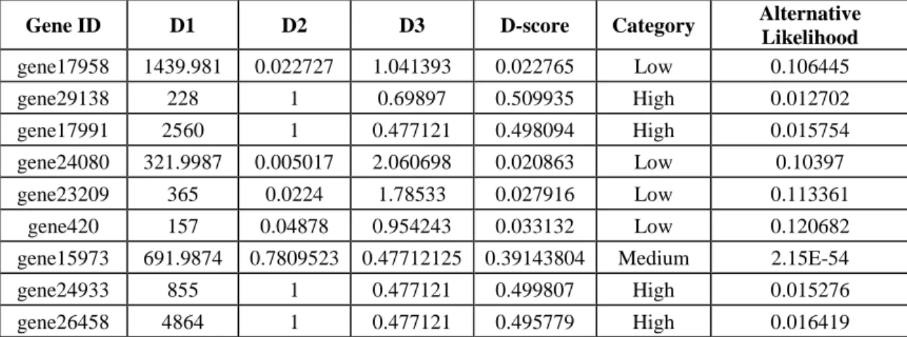
Table 2: GeneQC Example Output. The output of GeneQC from a Vitis vinifera sample, providing the extracted features, calculated D-score, mapping uncertainty categorization, and
alternative likelihood value.
Gene ID D1 D2 D3 D-score Category Alternative Likelihood gene17958 1439.981 0.022727 1.041393 0.022765 Low 0.106445 gene29138 228 1 0.69897 0.509935 High 0.012702 gene17991 2560 1 0.477121 0.498094 High 0.015754 gene24080 321.9987 0.005017 2.060698 0.020863 Low 0.10397 gene23209 365 0.0224 1.78533 0.027916 Low 0.113361 gene420 157 0.04878 0.954243 0.033132 Low 0.120682
gene15973 691.9874 0.7809523 0.47712125 0.39143804 Medium 2.15E-54
gene24933 855 1 0.477121 0.499807 High 0.015276
gene26458 4864 1 0.477121 0.495779 High 0.016419
2.1.3 Application on Real Data
In order to display the use of GeneQC, one dataset from each of the seven species were investigated for multi-mapping issues (Table 3). Based on this analysis, it is evident that plant samples tend to have higher proportions of genes with mapping uncertainty than animal samples (Figure 6). These results correlate with the fact that plant genomes tend to have higher levels of duplication, which is a strong contributing factor to mapping
uncertainty. While H. sapiens and M. musculus have lower proportions of genes with
mapping uncertainty than the plant samples, the proportion of genes with high mapping uncertainty of all the genes with mapping uncertainty is much higher. Plant species exhibited mapping uncertainty in an average of 12.6% of genes across the five species, whereas animal species exhibited this issue in an average of 5% of genes. However, over half of the genes with mapping uncertainty in the animal samples fall into the “High” categorization, while only around one-fifth of genes with mapping uncertainty from plant
samples fall into this category. The contributing factors to the higher proportion of “High” categorized genes for animal samples can be seen when looking at the three extracted features for each species.
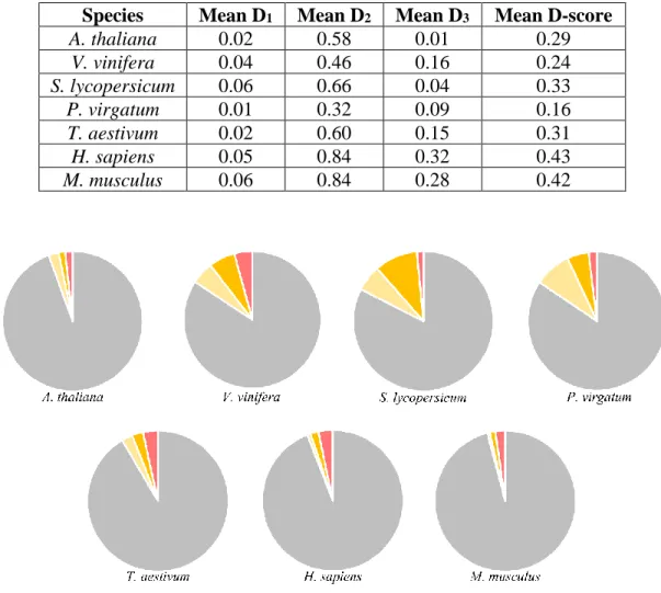
Table 3: GeneQC Analysis of Seven Species. This table shows the sample ID and relevant
metrics for each of the seven datasets analyzed. Mean values for D1, D2, D3, and D-score are calculated based on the genes that exhibit some level of mapping uncertainty, and D1, D2, and D3 were normalized for comparison.
Species Mean D1 Mean D2 Mean D3 Mean D-score
A. thaliana 0.02 0.58 0.01 0.29 V. vinifera 0.04 0.46 0.16 0.24 S. lycopersicum 0.06 0.66 0.04 0.33 P. virgatum 0.01 0.32 0.09 0.16 T. aestivum 0.02 0.60 0.15 0.31 H. sapiens 0.05 0.84 0.32 0.43 M. musculus 0.06 0.84 0.28 0.42
Figure 6: The categorization results related to the analysis of seven datasets representing five
plant and two animal species indicating level of mapping uncertainty per gene are shown relative to all categorizations.
The analysis results for the three features and calculated D-scores for genes with some level of mapping uncertainty are displayed in Figures 7 and 8, respectively. Both
H. sapiens and M. musculus display higher levels of sequence similarity (D1), shared MMR proportion (D2), and degree (D3) than what is generally exhibited in the analyzed plant species. These relatively high values for each feature led the higher D-scores, translating to a higher measure of mapping uncertainty in the animal samples compared
with the plant samples. Mean D-score for H. sapiens and M. musculus are 0.43 and 0.42,
respectively. These average values are much higher than those for the analyzed plant
samples, which are 0.29, 0.24, 0.33, 0.16, and 0.31 for A. thaliana, V. vinifera, S.
lycopersicum, P. virgatum, and T. aestivum, respectively.
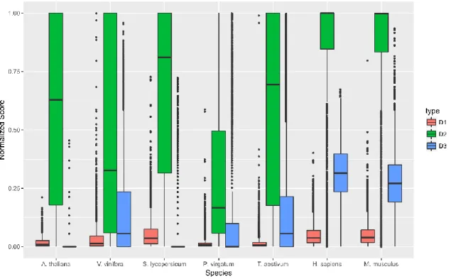
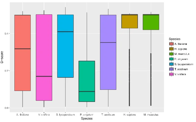
Figure 7: Boxplots results of the seven analyzed species using GeneQC for the three extracted
features of each gene. D1, D2, and D3 represent the sequence similarity, proportion of shared MMR, and degree weight, respectively. Each value is shown normalized between 0 and 1. Only
Figure 8: Derived D-scores for each gene are shown by species for each of the seven analyzed datasets, as calculated from the three features in Figure 7. Higher D-scores represent higher
levels of mapping uncertainty.
2.1.4 Summary
GeneQC is a tool used to investigate the prominent issue of mapping uncertainty in modern RNA-Seq analysis. Oversight in the quality of derived gene expression estimates based on mapping results can have drastic consequences for all downstream analyses and read mapping uncertainty is a significant cause of problems in further analysis. While read mapping has been accepted as sufficient, entirely ignoring the possibility of poorly mapped reads used for further analysis can have detrimental effects on all manner of RNA-Seq studies. As demonstrated in our analysis of 95 RNA-Seq datasets, the problem of mapping uncertainty is prominent and is displayed directly in the gene expression estimates. GeneQC can provide insight into the severity of this issue for each annotated gene along with a statistical evaluation framework. It utilizes feature
extraction, elastic-net regularization, and mixture model fitting to provide researchers with a sense of the quality of gene expression estimates resulting from the read alignment step. GeneQC provides sufficient information for researchers to make more
well-informed decisions based on the results of their RNA-Seq data analysis and to plan further analyses to address mapping uncertainty.
The application of GeneQC on the seven analyzed datasets display some interesting differences between plant and animal samples. Fewer genes displayed
mapping uncertainty in the animal samples, while a higher proportion of these genes were categorized as “High”. Alternatively, a much higher proportion of plant genes displayed mapping uncertainty, but more of these genes had moderate to low mapping uncertainty, relative to genes from animal samples. Both of these scenarios display the severity of mapping uncertainty in modern RNA-Seq analyses. High mapping uncertainty displayed in animal samples can lead to very biased expression estimates over fewer genes, while moderate levels of mapping uncertainty on a wider scale as displayed in plant species can cause widespread expression estimate biases on a lesser scale.
Not only does GeneQC provide a method for analyzing the severity of mapping uncertainty in analyzed data, it also enables researchers to directly compare the
expression estimates generated by various alignment tools using real world data. While current comparisons rely on large-scale simulated data—which fails to accurately capture the biological complexities of real RNA-Seq data—or small-scale real data using qPCR or the limited validated gene sets, GeneQC allows for any type of real data to be used to directly compare alignment strategies through the use of D-scores and categorization percentages.
2.2 ARM: Ambiguous Read Mapping Algorithm
While GeneQC provides a direct framework to determine the severity of mapping uncertainty and reliability of expression estimates, addressing these issues involves application of a different approach. Current alignment tools mainly consider local information in the context of the reads and reference genomes. While the strategies implemented by these tools are of high quality relative to the information used, they are still not suitable to provide optimal alignment results, since there are still serious issues related to the reliability of alignment results as demonstrated in Section 2.1. One approach that could rectify this issue is to consider a wider scope of information. In particular, using pathway and regulatory information can provide a new level of information to consider when aligning reads.
Transcription factors are proteins that bind to specific DNA sequences and play
important roles in controlling the expression levels of their target genes. Cis-regulatory
motifs are short, conserved segments of DNA and are typically binding sites for these transcription factors [94]. These binding sites play significant roles in regulating the rate of transcription for nearby genes. Hence, prediction of transcription factor binding sites provides a solid foundation for inferring gene regulatory mechanisms and building regulatory networks for a genome [95-98].
In order to determine more accurate expression estimations, I present an algorithm for ambiguous reads mapping (ARM). ARM integrates information in the form of
metabolic pathways, regulatory networks, alignment locations, and reads counts to provide negative binomial distribution-based re-alignment leading to more accurate expression estimates from RNA-Seq data (Figure 9).
Figure 9: ARM Algorithm Framework. KEGG Pathways are analyzed using the BOBRO motif prediction tool to develop networks of co-regulated genes (CRGs). Simultaneously, GeneQC
extracts information related to potential alignment locations for each read, along with unambiguous read counts. The unambiguous read counts are used along with proportional ambiguous read counts for each CRG network to generate a negative binomial-based distribution
for each potential alignment location. Based on the current read count of the potential gene location, a probabilistic alignment for each ambiguous read is determined.
2.2.1 Methods
ARM relies on key pieces of information from multiple sources to determine a sounder alignment of ambiguous reads. First, ambiguous reads are determined through GeneQC as any reads belonging to genes with particular levels of mapping uncertainty. By default, any reads aligned to genes falling into the “High” or “Medium” mapping uncertainty categorizations are considered ambiguous reads; although, reads from genes falling into the “Low” categorization could be considered also.
In addition to the qualification of ambiguous reads, GeneQC also provides
information related to potential alignment locations and read counts. For each ambiguous read, a modified version of GeneQC provides a list of potential alignment locations based on the initial alignment results. Furthermore, GeneQC extracts ambiguous and
unambiguous read counts for each potential alignment location. The unambiguous read counts are calculated as the total number of reads that are uniquely mapped to that particular location, while the unambiguous read counts are the total number of reads that are mapped to that location but could be mapped to another location.
Co-regulatory networks are determined by integration of pathway information and motif prediction. First, KEGG metabolic pathways [99] are collected for the specific species of interest. Each of these pathways are separately analyzed using DMINDA2.0 [100] with the backend algorithm being BOBRO [101] for motif prediction. The genes that are regulated or targeted by these predicted motifs create a single co-regulatory network, as co-regulated gene modules tend to have more similar expression patterns; hence, these modules can be used to train the re-alignment model.
For each ambiguous read, the potential alignment locations are isolated with their corresponding co-regulatory networks to develop a series of distributions. Read count distributions have widely been understood to follow negative binomial distributions [34,
36, 102, 103]. Following this framework, the distribution for read counts of gene j can
then be represented using a negative binomial distribution denoted as 𝑋𝑗~𝑁𝐵(𝑟, 𝑝),
following the probability mass function of
𝑃(𝑋 = 𝑘) = (𝑘 + 𝑟 − 1
𝑘 ) 𝑝
This formulation represents the probability of achieving the 𝑘𝑡ℎ success on the
𝑟 + 𝑘 = 𝑛𝑡ℎ attempt, with the independent probability of a success being 𝑝. While this does not have direct applicability or interpretability within the scope of read counts, a conversion can shed more light. The expected value and variance of the read count of
gene j are respectively calculated as 𝜇𝑗 = 𝐸(𝑋𝑗) = 𝑝𝑟
1−𝑝 and 𝜎𝑗
2 = 𝑉𝑎𝑟(𝑋 𝑗) =
𝑝𝑟 (1−𝑝)2
[104]. Thus, with some basic algebra, we obtain the following:
𝜇𝑗 = 𝑝𝑟 1 − 𝑝→ (1 − 𝑝)𝜇𝑗 = 𝜇𝑗− 𝑝𝜇𝑗 = 𝑝𝑟 → 𝜇𝑗 = 𝑝𝑟 + 𝑝𝜇𝑗 = 𝑝(𝑟 + 𝜇𝑗) → 𝑝 = 𝜇𝑗 𝑟 + 𝜇𝑗 → 1 − 𝑝 = 1 − 𝜇𝑗 𝑟 + 𝜇𝑗 = 𝑟 𝑟 + 𝜇𝑗
Using this information, an alternative formulation of the probability mass function can be derived as:
𝑃(𝑋 = 𝑘) = (𝑘 + 𝑟 − 1 𝑘 ) 𝑝 𝑘(1 − 𝑝)𝑟= (𝑘 + 𝑟 − 1 𝑘 ) ( 𝜇𝑗 𝑟 + 𝜇𝑗 ) 𝑘 ( 𝑟 𝑟 + 𝜇𝑗 ) 𝑟 = (𝑘 + 𝑟 − 1)! 𝑘! (𝑟 − 1)! ( 𝜇𝑗 𝑟 + 𝜇𝑗) 𝑘 (𝑟 + 𝜇𝑗 𝑟 ) −𝑟 =Γ(𝑘 + 𝑟) 𝑘! Γ(𝑟) ( 𝜇𝑗 𝑟 + 𝜇𝑗) 𝑘 (1 +𝜇𝑗 𝑟) −𝑟
where Γ is the gamma function defined as
Γ(𝑦) = ∫ 𝑥𝑦−1𝑒−𝑥𝑑𝑥 ∞
0
From this formula, we can estimate 𝜇𝑗 using 𝜇̂𝑗 = 𝑥̅ and 𝑟 using 𝑟̂ = 𝑥̅2
𝑠2−𝑥̅, where
𝑥̅ is the sample mean and 𝑠2 is the sample variance [105]. With this estimation, we can
represent the probability mass function of read counts as
𝑃(𝑋 = 𝑘) = (𝑘 + 𝑟̂ − 1 𝑘 ) ( 𝜇̂𝑗 𝑟̂ + 𝜇̂𝑗) 𝑘 ( 𝑟̂ 𝑟̂ + 𝜇̂𝑗) 𝑟̂ = (𝑘 + ( 𝑥̅2 𝑠2− 𝑥̅) − 1 𝑘 ) ( 𝑥̅ 𝑥̅2 𝑠2− 𝑥̅+ 𝑥̅ ) 𝑘 ( 𝑥̅2 𝑠2 − 𝑥̅ 𝑥̅2 𝑠2− 𝑥̅+ 𝑥̅ ) 𝑥̅2 𝑠2−𝑥̅
Using this distribution framework, ARM calculates the sample mean 𝑥̅ and
sample variance 𝑠2 for each co-regulatory network.
For a given read i, a set of n potential alignment locations is provided through
GeneQC. Each of the n potential locations has a co-regulatory network with a calculated
𝑥̅ and 𝑠2. ARM calculates the alignment value of read i to gene location j as
𝐴𝑖,𝑗 = 𝑃(𝑋 ≤ 𝑥̅) − 𝑃(𝑋 ≤ 𝑘𝑗+ 1)
where 𝑘𝑗 = 𝑢𝑗 + 𝑟𝑜𝑢𝑛𝑑(𝑐𝑗𝑎𝑗), with 𝑢𝑗 representing the unique read count, 𝑎𝑗
representing the ambiguous read counts, 𝑐𝑗 = max {0, 1 − 2𝐷𝑗} representing the
ambiguous count weighting factor, and 𝐷𝑗 representing the D-score calculated using
GeneQC. The weighting factor is used to give partial credit for ambiguously aligned reads for genes that have relatively low D-scores. Genes with high D-scores—those
close to 0.5—will be given little to no credit for ambiguously aligned reads. Read i will
alignment, the unique reads count 𝑢𝑗 for potential location j is updated. This process will be repeated for each ambiguous read.
2.2.2 Application on Real Data
In order to investigate the effectiveness of the ARM algorithm on re-alignment of ambiguous reads, GeneQC was used. In particular, the pre- and post-ARM D-scores
were evaluated for Vitis vinifera, Arabidopsis thaliana, Homo sapiens, and Mus musculus
to determine if ARM had any appreciable or statistical effect on mapping uncertainty. D-scores for each gene with some level of mapping uncertainty were calculated based on
the re-alignment using the ARM algorithm. Since D1 represents sequence similarity that
would not change with re-alignment, only D2 and D3 values changed. The same model
used to determine D-scores for the initial alignment was used to reflect an accurate change in the alignment quality. D-score distributions for genes with original non-zero D-scores are shown in Figure 10.
Figure 10: D-scores for the Pre- and Post-ARM algorithm for V. vinifera, A. thaliana, H. sapiens,
and M. musculus. Genes included in the generation of this figure had Pre-ARM D-scores greater
than zero, indicating some level of mapping uncertainty existing after initial alignment. Based on Figure 10, the effect of ARM on D-scores appears to be relatively minor overall. To more rigorously evaluate the effectiveness of the ARM algorithm, a paired Wilcoxon signed-rank test was used. This test acts as a nonparametric version of a paired t-test to determine if there is a difference in the pre- and post-ARM D-score pairings. A
significance level of 𝛼 = 0.10 was chosen to determine if significant improvements are
observed. This analysis generated 𝑝 − 𝑣𝑎𝑙𝑢𝑒 < 2.2𝑒−16 for V. vinifera, H. sapiens, and
M. musculus samples, thus indicating a statistically significant difference in D-scores due
to the ARM algorithm. For A. thaliana, the generated p-value is 0.0596. Based on this,
it is safe to conclude that the ARM re-alignment algorithm significantly improves D-scores. Figure 11 displays the percent of genes that observed improvements in D-score
through the use of the ARM algorithm. Overall, V. vinifera saw an improvement in
D-scores for 2.08%, A. thaliana saw an improvement in 0.02%, H. sapiens saw an
the ARM algorithm is specifically for re-alignment of ambiguous reads, it is more appropriate to view the performance of ARM relative to only the genes with some level of mapping uncertainty (i.e. D > 0). Based on these metrics, an improvement in 13.25%,
0.33%, 5.93%, and 25.93% of genes for V. vinifera, A. thaliana, H. sapiens, and M.
musculus was observed, indicating a relatively large proportion of improvement. The
ARM algorithm appears to be less effect for the A. thaliana sample than the others, which
is most likely due to the relatively limited network information generated through motif prediction.
Figure 11: Percent of Genes with Improved D-scores by species. The percent of genes that
observed an improved D-score through the ARM algorithm are displayed here. The red bar indicates the percentage relative to all genes, while the blue bar is with respect to the genes that had some level of mapping uncertainty to begin with (i.e. D > 0).
Additionally, of some importance is the degree to which the D-scores changed. If
D-scores improved for 25% of M. musculus genes but that change was very minor, the
the magnitude of impact, mean percent change and percent of genes that changed
mapping uncertainty categorization as a result of the ARM algorithm. Figure 12 displays
the mean percent change of D-score for the four species. Overall, the mean change for V.
vinifera, A. thaliana, H. sapiens, and M. musculus are 9.77%, 0.28%, 5.61%, and
24.42%, respectively. When considering the mean percent change only for the genes that exhibited some change in D-score as a result of the ARM algorithm, these numbers
increased to 75.64%, 85.4%, 95.47%, and 94.18%, respectively. Again, A. thaliana has a
lower overall metric than the other species, which is potentially due to the limited network information. This theory is supported by the similar mean percent difference when considering only genes that showed some difference in post-ARM D-score.
Figure 12: Mean percent change in D-score by species. The red bar indicates percent change
overall genes, while the blue indicates mean percent change for genes that exhibited some change in D-score.
Impact for the ARM algorithm can also be observed through the percent of genes