Rejoinder to ‘Post-selection shrinkage estimation for high-dimensional data analysis’ By: Xiaoli Gao, S. Ejaz Ahmed, Yang Feng
This is the peer reviewed version of the following article:
Gao, X.L., Ahmed, S.E. and Feng, Y. (2017). Rejoinder: Post Selection Shrinkage Estimation for High Dimensional Data Analysis. Applied Stochastic Models in Business and Industry, 33(2), 131-135. doi: 10.1002/asmb.2245,
which has been published in final form at http://dx.doi.org/10.1002/asmb.2245. This article may be used for non-commercial purposes in accordance with Wiley Terms and Conditions for Self-Archiving
Made available courtesy of Wiley:
http://onlinelibrary.wiley.com/wol1/doi/10.1002/asmb.2245/full
***© Wiley. Reprinted with permission. No further reproduction is authorized without written permission from Wiley. This version of the document is not the version of record. Figures and/or pictures may be missing from this format of the document. ***
Abstract:
One fundamental ingredient of our work is to formally split the signals into strong and weak ones. The rationale is that the usual one-step method such as the least absolute shrinkage and selection operator (LASSO) may be very effective in detecting strong signals while failing to identify some weak ones, which in turn has a significant impact on the model fitting, as well as prediction. The discussions of both Fan and QYY contain very interesting comments on the separation of the three sets of variables. Regarding Assumption (A2) about the weak signal set S2, we admit that the original version was not as rigorous as it could have been, as it could have contained the variables in S3. We now propose the following Assumption (A2') that replaces (A2) in the original paper.
Keywords:mathematics | post-shrinkage estimation | high-dimensional regression | data analysis Article:
We sincerely thank all the discussants Kjell Doksum and Joan Fujimura (DF); Jianqing Fan (Fan); Peihua Qiu, Kai Yang, and Lu You (QYY); and Yanming Li, Hyokyoung Grace Hong, and Yi Li (LHL) for the thought-provoking and insightful discussions on our paper. We would also like to thank the Editor Fabrizio Ruggeri for processing and organizing the discussion. Ahmed would like to specially thank him for his encouragement on this paper and patience. 1 Strong signal, weak signal, and noise
One fundamental ingredient of our work is to formally split the signals into strong and weak ones. The rationale is that the usual one-step method such as the least absolute shrinkage and selection operator (LASSO) may be very effective in detecting strong signals while failing to identify some weak ones, which in turn has a significant impact on the model fitting, as well as
prediction. The discussions of both Fan and QYY contain very interesting comments on the separation of the three sets of variables. Regarding Assumption (A2) about the weak signal set S2, we admit that the original version was not as rigorous as it could have been, as it could
have contained the variables in S3. We now propose the following Assumption (A2') that replaces (A2) in the original paper.
(A2'): The parameter vector β∗ satisfies that for some 0<τ<1, where ∥·∥ is the ℓ2 norm and for any j∈S2.
QYY mentioned that in practice, it is sometimes difficult to have a subjective separation of strong and weak signals. First of all, we would like to emphasize that the conditions imposed in the paper are from an asymptotic point of view, which demonstrate the great performance of the proposed estimators in the specified scalings and covariance structure. Second, we would like to argue that this separation is sometimes unnecessary in practice as the ultimate goal of high-dimensional regression is to provide accurate predictions for future data after variable selection and insightful interpretations on the importance of the predictors in terms of explaining the response. Third, the separation of strong and weak signals was mainly used to stimulate the post-selection shrinkage estimation (PSE) method, and the variables identified as ‘strong’ or ‘weak’ by PSE do not necessarily have a natural separation in terms of true regression coefficients, at least for a fixed sample size.
2 Conditions on designed matrix
We thank Fan for pointing out that the assumption on the design matrix could be strong. In fact, condition (B2) is mainly motivated from [1], and it requires the weak signals to be correlated to strong ones, in order for it to be detectable using the weighted ridge regression. On the other hand, condition (B4) requires that the eigenvalues of the design matrix corresponding to both strong and weak signals are bounded away from both 0 and infinity. Now, we describe one specific example. Consider an n×p design matrix X=[X1,X2,X3]. X1 and X2 correspond to strong
and weak signals, and X3 includes noises. Suppose all signals in Z=[X1,X2] are correlated with
constant correlation coefficient of r and uncorrelated with noises in X3. Then, such a design
matrix satisfies both conditions (B2) and (B4). We agree that some reasonably correlated design matrix for all variables could be excluded under those conditions.
3 MUJI variables
We thank LHL for bringing up the marginally unimportant but jointly informative (MUJI) variable set [2], namely, ‘marginally unimportant but jointly important’ variables. Indeed, the inclusion of MUJI variables could significantly improve the performance of the vanilla sure independence screening approach [3]. However, we would like to argue that in our proposal, the estimation of S1 could be done by any variable selection method that could identify the strong
signals, for example, LASSO. As a result, S1 could already contain the MUJI variables as it
considers the joint regression on all predictors.
Motivated by the MUJI variables, LHL proposed a new shrinkage estimator called Covariance Insured Screening-based PSE (CIS-PSE), which uses two simulation examples to compare
HD-PSE and CIS-HD-PSE. They conclude that using MUJI can help to improve the risk performance of the shrinkage estimator. However, the comparison could be a little unfair because S1 in CIS-PSE
is generated by marginal correlation, while S1 in HD-PSE is from LASSO. Thus, S1 generated
from two methods can be different. To ensure a fair comparison, we let S1 in the first step from
both CIS-PSE and HD-PSE be consistent. We consider different scenarios: (i) S1 is selected by
LASSO; (ii) S1 is selected by the minimax concave penalty (MCP); (iii) S1 is selected using the
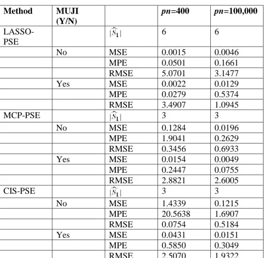
marginal strong set suggested by LHL in the first step while producing CIS-PSE. For each of those aforementioned three cases, we compute the MUJI set as suggested by LHL and then shrinking in the direction of . We define those three estimates as LASSO-PSE, MCP-PSE, and CIS-PSE, correspondingly. We then recheck those two examples, compare their performance, and report the results in Tables 1 and 2 ‡. When pn=100,000, we apply ridge regression and keep the 500 variables with the largest absolute coefficients before applying our algorithm.
Table 1. Simulated results for example 1 Method MUJI (Y/N) pn=400 pn=100,000 LASSO-PSE 6 6 No MSE 0.0015 0.0046 MPE 0.0501 0.1661 RMSE 5.0701 3.1477 Yes MSE 0.0022 0.0129 MPE 0.0279 0.5374 RMSE 3.4907 1.0945 MCP-PSE 3 3 No MSE 0.1284 0.0196 MPE 1.9041 0.2629 RMSE 0.3456 0.6933 Yes MSE 0.0154 0.0049 MPE 0.2447 0.0755 RMSE 2.8821 2.6005 CIS-PSE 3 3 No MSE 1.4339 0.1215 MPE 20.5638 1.6907 RMSE 0.0754 0.5184 Yes MSE 0.0431 0.0151 MPE 0.5850 0.3049 RMSE 2.5070 1.9322
Larger RMSE, smaller MSE, and smaller MPE indicate better performance. CIS, Covariance Insured Screening; MPE, mean prediction error; MSE, mean squared error; PSE, post-selection shrinkage estimation; RMSE, relative mean squared error.
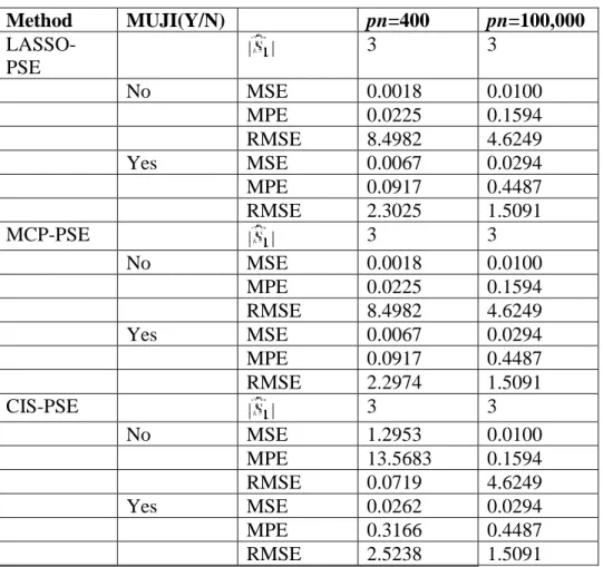
Table 2. Simulated results for example 2 Method MUJI(Y/N) pn=400 pn=100,000 LASSO-PSE 3 3 No MSE 0.0018 0.0100 MPE 0.0225 0.1594 RMSE 8.4982 4.6249 Yes MSE 0.0067 0.0294 MPE 0.0917 0.4487 RMSE 2.3025 1.5091 MCP-PSE 3 3 No MSE 0.0018 0.0100 MPE 0.0225 0.1594 RMSE 8.4982 4.6249 Yes MSE 0.0067 0.0294 MPE 0.0917 0.4487 RMSE 2.2974 1.5091 CIS-PSE 3 3 No MSE 1.2953 0.0100 MPE 13.5683 0.1594 RMSE 0.0719 4.6249 Yes MSE 0.0262 0.0294 MPE 0.3166 0.4487 RMSE 2.5238 1.5091
Larger RMSE, smaller MSE, smaller MPE indicate better performance. CIS, Covariance Insured Screening; MPE, mean prediction error; MSE, mean squared error; PSE, post-selection shrinkage estimation; RMSE, relative mean squared error.
In the tables, we report mean squared error and relative mean squared error. We also report the mean prediction error based upon the selected subset, defined as
In Example 1 in LHL, there is strong correlation among three covariates with weak signals and three covariates with strong signals. From the evaluation results reported in Table 1, we observe that when using the MCP-PSE and CIS-PSE, incorporating the MUJI variables improves the performance of the method as it can include additional signals from the MUJI set. However, when using LASSO-PSE, it is clear that using MUJI actually deteriorates the performance of the method by having larger mean squared errors and smaller relative mean squared errors. This is probably because LASSO already selects some weak signals in additional to the strong signals, which makes the MUJI detection step unnecessary. In Example 2 in LHL, there is strong correlation among three noise covariates and three covariates with strong signals. From the evaluation results reported in Table 2, we observe that both Lasso and MCP only select strong signals with no weak signals. Incorporating MUJI variables deteriorates the performances of
both MCP-PSE and LASSO-PSE in this case. This is because MUJI variables may pick up those noises in the second step. However, CIS-PSE with MUJI variables can help to improve the performance of the method.
From this preliminary numerical study, we can see that including MUJI variables may or may not improve the performance of the PSE, depending on the selected submodel.
The corresponding theoretical analysis regarding when the MUJI variables help the final estimation is an interesting open research question.
4 About the algorithm
DF suggested to use the partial least square method in the second step to select the weak signals, as opposed to the current weighted ridge regression. We appreciate the suggestion; however, one still needs to impose regularization on the estimates, which would lead to a different strategy and should be of interest for further research.
QYY posed the question about the selection of the tuning parameters an and rn in the PSE strategy. We agree that the proposed cross-validation method, while effective in our limited numerical experience, may need further theoretical justification. Recently, [4, 5] conducted a systematic study on the cross-validation-based tuning parameter selection method for high-dimensional penalized regression problems. Some work along similar lines could be an
interesting research project. In addition, it is also important to develop a certain adaptive tuning parameter selection method and demonstrate its robustness against model misspecification. 5 Future directions
This paper introduced the post-shrinkage estimation framework and used specific methods to select the strong and weak signals. The shrinkage estimation received a lot of attention since its inception decades ago. It strikes a balance between post-selected submodels and
high-dimensional weighted ridge estimators and is proved to be an effective strategy.
There are a number of alternatives to mimick the ideas of the PSE. For example, Fan suggested a great idea involving using the penalized least square with different penalty levels, closely related to the folded concave penalties including the smoothly clipped absolute deviations penalty (SCAD) and MCP.
The current methodology can be extended in a host of directions, including nonparametric models (suggested by QYY), spatially corrected data, among others. We would like to remark here that shrinkage estimation strategies have already been applied to some nonparametric models in low-dimensional cases such as [6-8], among others that can be extended to high-dimensional cases.
Another interesting direction would be to study the shrinkage method in robust high-dimensional data analysis, such as M-estimation. Recently, [9, 10] proposed penalized weighted least squares and penalized weighted least absolute deviation methods to study robust high-dimensional regression. The methods unify the M-estimation in a penalized weighted least squares and least
absolute deviation framework. Such a connection will enable us to extend the post-selection shrinkage strategy to robust high-dimensional regression models.
The scope of research in PSE is expanding. How to develop a system of diagnostic tools for the high-dimensional post-shrinkage estimators is an important direction for future research, as suggested by QYY.
Acknowledgements
Ahmed is supported by grants from NSERC. Gao is supported by Simons grant no. 359337. Feng is supported by NSF CAREER grant DMS-1554804.
‡ The results of LASSO-PSE and MCP-PSE are identical when pn=400 because they always select the same .
References
1 Shao J, Deng X. Estimation in high-dimensional linear models with deterministic design matrices. Annals of Statistics 2012; 40: 812–831.
2 Li Y, Hong H, Kang J, He K, Zhu J, Li Y. Classification with ultrahigh-dimensional features. arXiv preprint arXiv:1611.01541 2016.
3 Fan J, Lv J. Sure independence screening for ultra-high-dimensional feature space (with discussion). Journal of the Royal Statistical Society, Series B 2008; 70: 849–911.
4 Yu Y, Feng Y. Modified cross-validation for LASSO penalized high-dimensional linear models. Journal of Computational and Graphical Statistics 2014; 23: 1009–1027.
5 Feng Y, Yu Y. Restricted consistent cross-validation for tuning parameter selection in high-dimensional variable selection. manuscript2016.
6 Hossain S, Ahmed SE, Yi GY, Chen B. Shrinkage and pretest estimators for longitudinal data analysis under partially linear models. Journal of Nonparametric Statistics 2016; 28: 531–549. 7 Buhamra S, Al-Kandarri S, Ahmed SE. Nonparametric inference strategies for the quantile functions under left truncation and right censoring. Journal of Nonparametric
Statistics 2007; 19: 189–198.
8 Ahmed SE, Hussein AA, Sen PK. Risk comparison of some shrinkage M-estimators in linear models. Journal of Nonparametric Statistics 2006; 18: 401–415.
9 Gao XL, Fang Y. Penalized weighted least squares for outlier detection and robust regression. https: //arxiv.org/abs/1603.07427, 2016.
10 Gao XL, Feng Y. Penalize weighted least absolute deviation regression. Statistics and Its Interface 2017. Accepted for publication.