1-1-2016
Big Data Management Using Scientific Workflows
Andrii Kashliev
Wayne State University,
Follow this and additional works at:
https://digitalcommons.wayne.edu/oa_dissertations
Part of the
Computer Sciences Commons
This Open Access Dissertation is brought to you for free and open access by DigitalCommons@WayneState. It has been accepted for inclusion in Wayne State University Dissertations by an authorized administrator of DigitalCommons@WayneState.
Recommended Citation
Kashliev, Andrii, "Big Data Management Using Scientific Workflows" (2016).Wayne State University Dissertations. 1548.
by
ANDRII KASHLIEV
DISSERTATION
Submitted to the Graduate School of Wayne State University,
Detroit, Michigan
in partial fulllment of the requirements for the degree of
DOCTOR OF PHILOSOPHY
2016
MAJOR: COMPUTER SCIENCE
Approved By:
2016
To God be the glory.
I would rst like to thank God for giving me an amazing opportunity to pursue a Ph.D. degree in a fascinating eld of Computer Science, for giving me a passion to research, for bringing me to Wayne State University to work with my advisor Dr. Shiyong Lu, for guiding me through a number of important decisions, for protecting me, for answering my prayers, and for giving me the strength to persevere. I would also like to express my deep and sincere gratitude to my advisor Dr. Shiyong Lu, for his guidance, encouragement, and support throughout my Ph.D. studies. Dr. Lu's advice has enabled me to remain focused and to succeed in my studies. I am deeply thankful for Dr. Lu's kindness and for inspiring me to pursue an academic career. I am also very grateful to my dissertation committee members: Dr. Shiyong Lu, Dr. Alexander Kotov, Dr. Chandan K. Reddy, as well as Dr. Qiang Zhu in the Department of Computer and Information Science at the University of Michigan - Dearborn, for being on my dissertation committee and for providing their helpful feedback, insightful comments, and constructive suggestions.
I would also like to thank Dr. Fotouhi for his encouragement and support during my Ph.D. studies. I am deeply thankful for the University Graduate Research Fellowship award that has enabled me to have an early start in my Ph.D. research. I would also like to thank Dr. Artem Chebotko for his invaluable help for the past seven years, and for being an outstanding mentor, an inspiring role model, and a great collaborator. I would also like to thank my bright colleagues from the Big Data Research Laboratory: Dong Ruan, Fahima Bhuyan, Aravind Mohan, Mahdi Ebrahimi, and Scotia Roopnarine, as well as alumni Dr. Chunhyeok Lim, Dr. Cui Lin, and Dr. Xubo Fei.
I am especially thankful to my beautiful wife, who has been incredibly supportive throughout my studies. My deep gratitude goes to my loving parents, my sister, my brother-in-law and to my entire family.
Acknowledgements iii
LIST OF TABLES vii
LIST OF FIGURES viii
CHAPTER 1: INTRODUCTION 1
1.1 Problem Statement . . . 2
1.1.1 Scientic Workow Verication . . . 2
1.1.2 Shimming Techniques in Scientic Workows . . . 3
1.1.3 Scientic Workow Management in the cloud . . . 4
1.2 Main Contributions . . . 6
1.3 Organization . . . 7
CHAPTER 2: RELATED WORK 8 2.1 Scientic Workow Modeling . . . 8
2.2 Scientic Workow Verication . . . 11
2.3 Shimming Techniques in Scientic Workows . . . 13
2.4 Scientic Workow Management in the Cloud . . . 15
CHAPTER 3: SCIENTIFIC WORKFLOW VERIFICATION 17 3.1 Scientic Workow Model . . . 17
3.2 Workow Expressions . . . 21
3.3 Type System for Scientic Workows . . . 25
3.4 Subtyping in Scientic Workows . . . 27
3.5 Typechecking Scientic Workows . . . 34
3.6 Chapter Summary . . . 38
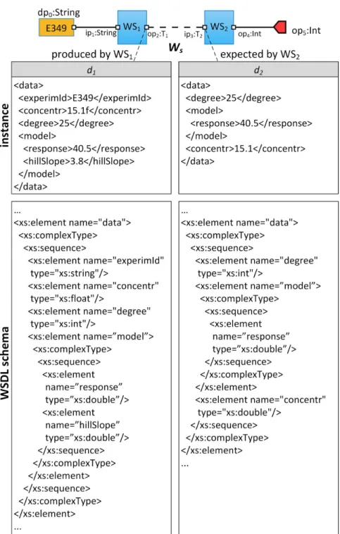
CHAPTER 4: A TYPETHEORETIC APPROACH TO SHIMMING 39 4.1 Motivating Example from the Biological Domain . . . 39
4.3.1 Primitive Shimming in Workow Wa . . . 48
4.3.2 Composite Shimming in Workow Ws . . . 49
4.3.3 Mediating Web Services from myExperiment Portal . . . 52
4.4 Chapter Summary . . . 52
CHAPTER 5: SCIENTIFIC WORKFLOW MANAGEMENT IN THE CLOUD 53 5.1 Big Data Challenges and Scientic Workows . . . 53
5.2 Main Challenges for Running Scientic Workows in the Cloud . . . 54
5.2.1 Platforms Heterogeneity Challenge . . . 55
5.2.2 Resource Selection Challenge . . . 56
5.2.3 Resource Utilization Challenge . . . 57
5.2.4 Resource Volatility Challenge . . . 60
5.2.5 Distributed Computing Challenge . . . 62
5.3 A System Architecture for BDWFMS in the Cloud . . . 63
5.4 Chapter Summary . . . 71
CHAPTER 6: DATAVIEW: BIG DATA WORKFLOW MANAGEMENT SYSTEM 73 6.1 DATAVIEW Implementation in the Cloud . . . 73
6.2 Case Study: Analyzing Driving Competency from Vehicle Data . . . 74
6.3 Case Study: Building Sky Image Mosaic . . . 77
6.4 Moving Big Data within the Cloud . . . 78
6.5 Chapter Summary . . . 79 CHAPTER 7: CONCLUSIONS AND FUTURE WORK 80 APPENDIX A: WDSL SPECIFICATION FOR THE WS1 WEB SERVICE 83 APPENDIX B: WDSL SPECIFICATION FOR THE WS2 WEB SERVICE 88
APPENDIX D: DATA PRODUCT LANGUAGE (DPL 2.0) 104
REFERENCES 110
ABSTRACT 122
AUTOBIOGRAPHICAL STATEMENT 124
Figure 3.1 Examples of scientic workows (Wa, Wb, ..., Wg). . . 19
Figure 3.2 The SWL specication of the workow Wa. . . 21
Figure 3.3 Two sample XSD types. . . 26
Figure 3.4 The subtyping DAG. . . 29
Figure 3.5 Subtyping inference rules. . . 30
Figure 3.6 Sample subtyping derivations. (a) Tphd <:Tgrad. (b) T1 <:T2from Ws. . . 31
Figure 3.7 Workow typing rules. . . 34
Figure 3.8 Typing derivation for workow Wa. . . 35
Figure 3.9 Typing derivation for workow Ws. . . 36
Figure 4.1 Sample Workow Ws. . . 40
Figure 4.2 Translating subtyping derivation into a composite coercion using translateS. . . 46
Figure 4.3 Automatically inserting primitive shim in workow Wa using the VIEW system. 48 Figure 4.4 The SWL specication of the workow with the shim automatically inserted. . . 49
Figure 4.5 Automatically inserting composite shim in workow Ws using the VIEW system. 51 Figure 5.1 Big data workow analyzing automotive data. . . 57
Figure 5.2 Montage workow for creating a mosaic of sky images. . . 58
Figure 5.3 A system architecture for BDWFMS in the cloud and its subsystems. . . 64
Figure 6.1 The graphical user interface of our DATAVIEW system. . . 74
Figure 6.2 Provisioning virtual machines in DATAVIEW. . . 75
Figure 6.3 Screenshot of the driving skill report from our big data workow in DATAVIEW. 76 Figure 6.4 Running big data workow from the automotive domain in Amazon EC2 cloud. 76 Figure 6.5 Moving 3Gb dataset to the target VM. . . 78
CHAPTER 1: INTRODUCTION
Humanity is approaching a new era, in which every sphere of our activity will be informed by big data. The amount of data in the world will continue to grow by 40% every year, from 4.4 zettabytes in 20131to 44 zettabytes in 2020 - enough to ll the memory of six stacks of iPads reaching from the Earth to the Moon [110]. Leveraging big data has the potential to revolutionize many areas of human activity, including scientic research, education, healthcare, energy, manufacturing, environmental science, urban planning, and transportation, just to name a few [111]. Examples of possible big data innovations may range from safer driving using connected vehicles to better fraud detection using machine learning, from energy-ecient homes with learning thermostats, to personalized medicine using wearable devices, from discovering new particles using Large Hadron Collider (LHC) to saving lives with remotely-monitored pacemakers. In the US healthcare alone, making use of big data can save an estimated 300 billion dollars annually [112].
However, making these breathtaking innovations a reality requires managing terabytes and even petabytes of data. For example, an average US company with over 1,000 employees typically has more than 200 terabytes of stored data [112]. Data are generated by billions of devices, products, and events, often in real time, in dierent protocols, formats and types. The volume, velocity, and variety of big data, known as the 3 Vs, present formidable challenges, unmet by the traditional data management approaches. Big data has become a critical research eld for the coming years. As a renowned database researcher and a recent Turing Award winner Michael Stonebraker puts it, I expect big data to be important for a long time to come.
Traditionally, many data analyses have been performed using scientic workows, tools for formalizing and structuring complex computational processes. A scientic workow provides a for-mal specication of a scientic process by capturing and streamlining all computational steps. It can be viewed as a data analysis pipeline, which incorporates a wide range of components, or tasks, such as data preparation tasks, data mining algorithms, scripts, local and remote software invoca-tions, Web services, visualization tasks, etc. A scientic workow management system (SWFMS) is a software system that allows users to design, store and execute scientic workows via a user-friendly graphical interface. SWFMS facilitates data analysis and scientic discovery by enabling
domain experts, such as physicists or biologists, to create, run, and manage their complex multi-step scientic data analyses. SWFMS provides necessary capabilities for managing scientic workows, including representation, serialization, and storage of workow specications that describe structure and congurations of workows and their constituent computational components. Other important functions of a SWFMS include workow composition, typically done via a drag-and-drop graphical interface, workow verication, scheduling, orchestration, data storage, and workow provenance collection. SWFMSs are used in a variety of domains, such biology, physics, chemistry, bioinformat-ics, and earthquake science [108, 109]. The intuitive and user-friendly interface of SWFMSs allows users with non-technical background to design and execute workows to extract knowledge from the data.
1.1 Problem Statement
While scientic workows have been used extensively in structuring complex scientic data analysis processes, little work has been done to enable scientic workows to cope with the three big data challenges on the one hand, and to leverage the dynamic resource provisioning capability of cloud computing to analyze big data on the other hand.
1.1.1 Scientic Workow Verication
Scientic workows have been an important paradigm for scientists to structure, integrate and execute complex multi-step computational pipelines that analyze and extract knowledge from data. As the volume, velocity, and variety of such data continues to grow, so does the complexity and size of scientic workows.
We argue that there is a pressing need to develop and implement a scientic workow verication technique. First, the growing size and complexity of scientic workows, as well as the increasing heterogeneity of workow components, make it increasingly dicult for users to ensure that there are no errors in the workow design. Indeed, when designing a large workow with dozens or even hundreds of heterogeneous components, the user may struggle to ensure 1) that all the required data channels are in place, 2) that all the required data products are properly connected to the appropriate workow components, 3) that there are no dangling input ports, and 4) every data channel links components that are syntactically compatible with each other, i.e., that the downstream component is capable of processing the data produced by the upstream component.
Second, running large-scale scientic workows often involves using large distributed computing resources, such as clouds [119, 121], whose cost can often be signicant. Indeed, an execution of a scientic workow analyzing big data in the cloud may last many hours or even days. Such executions are often terminated due to errors, e.g., an incorrect format of input data of one of the intermediate software components in the workow. Such errors result in a failure to nish execution, which often requires terminating virtual resources, correcting the errors in the workow design, provisioning a new set of virtual resources and re-running the entire workow, all of which adds additional expenses to and increases the time of the scientic experiment. To avoid needless expenses and to speed up scientic experiments, it is critical to determine whether the workow is correct and can execute successfully, before provisioning virtual resources and attempting to run the distributed workow in the cloud. Finally, although several large-scale scientic workow management systems have been proposed [12,80,83], a formal scientic workow verication technique is still missing.
1.1.2 Shimming Techniques in Scientic Workows
The variety of big data results in heterogeneity of data representation formats, data struc-tures, and the increasing number of services, such as WSDL services, with heterogeneous inter-faces. Such autonomous third-party services are often composed into scientic workows to perform eScience experiments to make discoveries in biology, chemistry, and other disciplines. However, very often, these services and applications are syntactically mismatching or semantically incompatible, necessitating the use of a special kind of workow components, called shims, to mediate them by performing appropriate data transformations. The shimming problem has been widely recognized as an important problem in the community [50, 51], leading to much eorts in the development of shims [48], shim-aware workow composition [50] and the suggestion of a new discipline called shi-mology [51]. Shims are ubiquitous, e.g., a study shows that shims constitute as much as 38% of all components used in bioinformatics workows on a popular myExperiment portal [52]. While shims are of no signicance to the actual domain problems being solved, shimming requires signicant eort, shims clutter workow design, and become a distraction from doing some real science [113]. Existing mediation techniques to insert shims have a number of limitations. First, exist-ing techniques are not automated and burden users by requirexist-ing them to generate transformation scripts, dene mappings to and from domain ontologies, and even write shimming code [47,53,54].
We believe these requirements are dicult and make workow design counterproductive for non-technical users. Second, current approaches produce cluttered workows with many visible shims that distract users from main workow components that perform useful work. Workow stud-ies [52, 55] show that the percentage of shim components in workows registered in myExperiment portal2 is at least 30%. These numbers indicate that such explicit shimming tends to make work-ows cluttered, which further diminishes the usefulness of these techniques. Third, many shimming techniques only apply under a particular set of circumstances that are hard to guarantee or even predict. Some approaches (e.g., [47,53,58, 59]) apply only when all the right shims are supplied by Web service providers and are properly annotated beforehand, and/or when required shims can be generated by automated agents (e.g., XQuery-based shims [58]), which cannot be guaranteed for any practical class of workows. Such uncertainty makes these techniques unreliable in the eyes of end users (domain scientists) who need assurance that their workows will run. Finally, while these eorts resolve structural dierences between complex types of Web services [47,53,59], they cannot mediate simple types, such as Int or Double.
Therefore, there is a pressing need for an automated and transparent approach to component mediation, or shimming, in order to simplify scientic workow composition and help scientists focus on solving their domain problems and making discoveries.
1.1.3 Scientic Workow Management in the cloud
Cloud computing oers on-demand access to vast amounts of storage and computing re-sources and exible pay-per-use pricing model. In the age of big data such unprecedented access to computing power makes cloud an essential paradigm, as it enables everyone, even small research teams, to dynamically build virtualized cyberinfrastructures for running their large-scale analytic workows in order to extract knowledge and value from big data. Without cloud, using big data would be a privilege only available to a handful of large corporations with massive IT budgets. In short, it is precisely cloud computing that makes it possible for most researchers and industry professionals to leverage big data.
Although scientic workows have been frequently utilized to formalize and structure com-plex data analyses, few attempts were made to enable scientic workows to leverage the elastic resources oered by cloud computing.
As an example, Fig. 1.1(a) shows a big data scientic workow from the automotive domain. Yellow and blue boxes represent data and tasks, respectively. The workow computes driver's competency from the vehicle data, that records, in small discrete steps, vehicle speed, steering wheel angle, brake pedal status, etc. Such information might be useful, for example to improve safety on the road by detecting incompetent drivers who need more training, or to assign lower auto insurance rates to safe drivers. As the average adult driver in the US may generate up to 75 gigabytes of such driving data annually, the total amount of data generated in the US may exceed 14 exabytes (1018 bytes) per year [104,114]. Another example, from the astronomy domain, is a Montage workow shown in Fig. 1.1(b), that reprojects and coadds sky images to create a mosaic. There are already many terabytes of such image les [115], and the scale of such astronomy workows will continue to grow. Running these data intensive workows requires using signicant computing resources oered by the cloud. Although several scientic workow management systems
Figure 1.1: Scientic workows from the (a) automotive and (b) astronomy domains.
(SWFMSs) have been developed to use cloud resources, most of them are geared either towards a specic domain, such as Tavaxy for bioinformatics [116], or towards a particular type of workows, such as SwinDeW-C system for QoS-annotated workows [117]. Besides, existing systems do not address the bottleneck of moving large datasets between virtual machines during workow execution in the cloud, which prolongs workow execution due to volume of big data and limited network bandwidth. Most importantly, a generic system architecture for running big data workows in the cloud is still missing.
1.2 Main Contributions
To address the aforementioned challenges, in this dissertation we make the following contri-butions:
• A Formal Approach to Scientic Workow Verication. We dened a scientic
work-ow model and shwork-owed that scientic workwork-ows are equivalent to typed lambda calculus expressions. We designed an algorithm, called translateWorkow to translate a scientic workow into an equivalent lambda expression. Next, we have introduced the notion of subtyping in scientic workows, along with the subtype relation, and dened a well-typed workow. Our notion of well-typed workow serves as a formal criterion for verifying scientic workows, and for knowing whether it is safe to execute a given scientic workow. We have also designed two algorithms, subtype and typecheckWorkow, that check whether two types belong to the subtype relation, and whether a workow is well-typed, respectively. We have implemented all of our proposed models, algorithms, and functions, as well as typed lambda calculus and type system in our scientic workow management system, called VIEW.
• A Typetheoretic Approach to the Shimming Problem in Scientic Workows. We
reduced the shimming problem from the eld of scientic workows to a runtime coercion problem in the theory of type systems. We dened a function translateS that generates co-ercions, or shims, that coerce (transform) data products into appropriate target data types. Next, we dened a function translateT, that translates a workow typing derivation into an expression, in which subtyping is replaced with runtime coercions, thereby resolving the shim-ming problem automatically. Finally, we implemented our automated shimshim-ming technique, including all the proposed algorithms, formalisms, and translation functions in our VIEW system and presented two case studies to validate our approach.
• A Reference Architecture for Running Big Data Workows in the Cloud. We
identied the key challenges for running big data workows in the cloud, based on a thorough literature review and our experience in using the cloud infrastructure. We then proposed a generic implementation-independent system architecture that addresses these challenges. We also proposed a data movement technique that leverages Elastic Block Store (EBS) volumes to transfer data across virtual machines in the cloud.
• DATAVIEW: Big Data Workow Management System. We developed a
cloud-enabled big data wofklow management system, called DATAVIEW that delivers a specic implementation of the proposed architecture. To validate our proposed architecture we con-ducted a case study in which we designed and ran a big data workow in the automotive domain using the Amazon EC2 cloud environment.
1.3 Organization
The rest of this dissertation is organized as follows: Chapter 2 presents related work on the current research in scientic workow verication, shimming techniques, and cloud-enabled workow system architectures. Chapter 3 presents our proposed technique for scientic workow verication. Chapter 4 presents our automated approach to shimming in scientic workows. Chapter 5 presents our proposed reference architecture for running big data workows in the cloud. Chapter 6 presents our cloud-enabled big data workow management system (BDWFMS), called DATAVIEW, along with our case study from an automotive domain.
CHAPTER 2: RELATED WORK
The importance of scientic workows for advancing data-intensive science has been widely recognized by the research community [1,2,4,8891]. This chapter introduces models and techniques that are most relevant to the approaches and solutions presented in this dissertation, most notably those concerning workow verication, workow shimming, and workow execution in the cloud. Workow verication is tightly coupled with the underlying workow model, which serves as a foundation for reasoning about workows. Therefore, we begin this chapter by discussing various scientic workow models in Section 2.1. Next, in Section 2.2 we discuss current approaches to workow verication. In Section 2.3 we present existing techniques to the shimming problem, which arises when linking together related but incompatible components. Finally, we discuss current approaches to executing scientic workows in cloud environments in Section 2.4.
2.1 Scientic Workow Modeling
Scientic workows [1, 3] facilitate discovery by allowing domain researchers design and execute complex computational processes, which consist of various local and remote computational resources, such as Web services, grid services, cloud resources, and local applications. Given the complexity of such processes, the task of modeling scientic workows becomes a non-trivial one. In this chapter we present ideas and approaches proposed and used by the research community to model scientic workows.
Taverna workows [4] are captured using an XML-based workow language, called Simple Conceptual Unied Flow Language (Scu) [7], which is dened using the computational lambda calculus. A Scu workow is a network of processors (or nodes) connected using data links. There may also be input and output ports, as well as coordination constraints for relationships between processors that are not enforced by data links [8]. [9] formalizes the workow composition using a sequent calculus. It denes a set of rules by which Taverna workows are composed.
Kepler is a workow management system, that allows scientists to capture workows in a format that can be easily exchanged, archived, versioned and executed [5, 10]. Kepler is built on top of Potlemy II system, which focuses on module-oriented, visual programming. Ptolemy II follows actor-oriented modeling paradigm. Workow is dened as a composition of independent actors, that communicate through ports. Actors are connected to each other via channels. The
execution model is dened by the director and is called the model of computation. There are a number of models used in Kepler, e.g. Process Networks (PN), Discrete Event systems (DE), etc. Thus, component interaction is dened by the directors, rather than by actors. Actor's behavior is thus determined by the model of computation of a director managing a particular composition of actors (behavioral polymorphism). As described in [11], Ptolemy II (and thus Kepler) also supports data polimorphism. For instance, PLUS operator may be implemented in a way that enables it to dynamically choose correct addition (double, integer, oat), given a concrete set of inputs, (or if inputs are string PLUS operator may even perform concattenation, etc). Another aspect of Kepler composition is hierarchical modelling. This is achieved using sub-workows (composite actors). A user can view the content of a sub-workow by right-clicking on its graphical representation and selecting Look inside.
Pegasus is a workow management system primarily focused on mapping an abstract speci-caiton of a scientic workow to the Grid and cloud resources [12]. The abstract workow (AW) is modeled as Directed Acyclic Graph (DAG) that captures workow components (called jobs in Pegasus terminology), their inputs and outputs, and all the data dependencies between the jobs. The serialization format used in Pegasus for abstract workow is an XML le, termed DAX, that conforms to the DAX XML schema [13]. Pegasus provides a number of ways for users to create DAX workow specication. These include composing workow directly, using DAX Schema, using DAX Python API, and using Chimera system [14] that takes as input partial logical workow descriptions specied by the user in Virtual Data Language (VDL) [14] and produces an abstract workow spec-ication. Finally, workows can be designed using Composition Analysis Tool (CAT) [15], which provides an interactive mechanism for scientist to incrementally compose a workow. The tool as-sists user during the workow composition by making suggestions every step of the way. To achieve this, the CAT tool relies on knowledge base that consists of Domain and Component Ontologies. While the former captures the hierarchy of data types involved in the domain, the latter contains workow components, expressed in terms of their input and output parameters data types. CAT supports workow components with varying degrees of detail. For instance, while Car-Rental-by-Airport workow produces Car-Reservation given an airport and a date, Car-Rental workow does the same, except that it takes location instead of airport as one of its inputs, which is more generic.
If during the composition planner nds multiple equally matching components to be inserted in certain slot of the workow, it suggests adding the most abstract component from that set. For example, planner may choose abstract ight reservation service, instead of suggesting a particular service, such as Expedia or Orbitz. For search and reasoning purposes, the knowledge base sup-ports a set of queries, such as, components(), which returns a set of available components from the knowledge base. Workow composition is seen as a sequence of steps performed by the user. After each step the system computes possible next steps and suggest them to the user. To analyze such partial workows the system utilizes AI planning techniques. Desired end results provided by the user are the goals of the planning problem. In CAT, each workow is a tuple<C, L, I, G>where C, L, I and G represent workow components, links, initial input components provided by the user and goals (end-result components). The initial inputs and end-results are treated as components with no inputs and no outputs respectively. Through this interactive process, user and the system together search the space of workows, with the goal of moving towards the subspace of correct workows. Authors of [15] point out that this interactive semi-automated approach is a balance between two extremes - manual workow composition (slow, inecient) and fully automated com-position (requiring the user to know and specify the exact goals at the very beginning, and leaving no room for the user to inuence workow design during the composition process).
Vistrails is a system that was designed to support exploratory computational tasks such as visualization and data analysis [16,92,93,96]. In Vistrails, a workow is composed via graphical user interface using drag and drop approach. Workows are represented using XML-based language that species all modules and connections between modules. VisTrails maintain a database of such XML workow specications, that users can query using XML query language such as XQuery to nd workows suitable for their tasks [17]. VisTrails workows can be executed by The Vistrail Player (VP), that takes as input an XML-based specication of the workow. In a VisTrails workow, each module may represent simple script, VTK module or web service. Vistrails allows to cluster workow components into groups and subworkows. Groups and subworkows can be subsequently used in other workows as building blocks.
Triana is a Problem Solving Environment that provides a user portal for the composition of scientic applications [18, 19]. According to [20], its distinct feature is the support of both a
composition environment and a mechanism for the distribution of components. Triana requires existence of Triana execution environment on each machine that executes a workow, or part of the workow. Although Triana uses its own XML-based language to represent workows, it supports external languages, including BPEL4WS. Each workow consists of components. Each component is an atomic unit of execution. A component may be a single algorithm or a process. Inputs of a component can be congured to be optional or mandatory. Availability of all mandatory inputs triggers component execution. Triana provides a graphical interface that allows users to compose workows by dragging and dropping programming components (referred to as units or tools in Triana terminology) onto the work surface and connecting them together [20].
Although all the systems described above allow to create and execute scientic workows in one form or another, each of these tools was developed to address a particular, more specic need. This fact resulted in slightly dierent architectures, user interfaces and sets of supported features. Taverna, for example was created to help bioinformatics research and support collabo-ration between domain scientists by allowing them to create and share reusable components. It thus provides extensive support for web services, and provides intuitive user-friendly graphical user interface. VisTrails workow system enables ecient execution of multiple visualization pipelines and provenance maintenance. Swift, on the other hand, focuses on allowing user to execute complex computations over large datasets (tens and hundreds of thousands of tasks and data les) on dis-tributed resources. Kepler was designed to be generic enough to support wide variety of workows, such as knowledge discovery, experiment automation, and experiment managgement and scheduling on high performance computing (HPC) environments. Kepler provides seamless access to web and grid services. Pegasus' major focus is on creation large workows with thousands and even millions of tasks that can be executed in distributed environments, such as grids and clouds.
2.2 Scientic Workow Verication
Workow verication is regarded as an important research direction by the research com-munity [22,24,28]. Verication was considered both at the system level, and at the theoretical level. We now discuss representative works on workow verication.
Scientic Workow Management Systems (SWFMSs) employ a range of techniques to verify workows. Pegasus system provides the CAT tool [15] as an interactive means for the user to
design a workow. As the user incrementally builds the workow, the tool provides assistance by detecting errors and making suggestions how to x them. The errors are detected using the knowledge base, which consists of Domain and Component Ontologies. During such analysis, the system takes into account input data provided by the user, component parameter data types, links between components in the partial workow etc. For search and reasoning purposes, the knowledge base supports a set of queries, including the following:
• components(): returns a set of available components from the knowledge base • data-types(): returns a set of data types
• input-parameters(c): returns input parameters of component c
• output-parameters(c): given a component c, returns a set of output parameters • output-parameters(c): given c, returns output patameters
• executable(c): returns false i c is not an executable component.
• range(c, p): returns a class dened as the range of parameter p of component c.
• subsumes(t1,t2): returns true of class t1 subsumes t2 in knowledge base. E.g. subsumes(location,
airport) = true, subsumes(airport,location) = false.
• component-with-output-data-type(t): returns a set of components such that each comopnent
has at least one output of type t (or one that subsumes t)
• component-with-input-data-type(t): returns a set of components, such that each component
has at least one input of type t (or one that subsumes t) The CAT tool considers various workow properties, such as:
• All inputs of all non-initial components are connected to some other components. In
CAT-terminology such workow is said to be satisifed.
• Data type of each output is consistent with the input of next component it is connected to.
Such link is said to be consistent.
• Each component's output is used (directly or indirectly) to produce the end result (in other
words, it contributes to the workow goal, as opposed to doing useless work). Such component is said to be justied.
• There is at least one goal dened by the user in the workow, i.e. workow is purposeful. • All components in the workow are executable. Such workow is called grounded.
After each step by the user, the system determines which properties are violated by running an algorithm, called ErrorScan [15].
[20] discusses Triana problem solving environment. The authors report that programming units in Triana workows contain type information for every port, that is used to check type com-patibility at design type. However, [20] does not discuss how typechecking is performed, i.e. does not present algorithms or a type system.
Existing theoretical studies focus primarily on control-ow [126, 127], temporal [128], and authorization constraints [127,129,130]. In [21] Cao et al. propose a state Pi calculus which enables modeling and temporal verication of grid workows. The authors only focus on the temporal prop-erties verications on the grid scientic workows. Choi et al. [22] presented a structural verication approach for cyclic workow models by means of acyclic decomposition and loop reduction.
While the above works discuss workow verication based on the user-dened goals [15], temporal constraints [21], and structural properties [15, 22], more research is needed to formally dene and reason about well-typedness of scientic workows. In addition, algorithms to verify such well-typedness are needed to ensure successful workow execution.
2.3 Shimming Techniques in Scientic Workows
The variety of big data results in heterogeneity of data representation formats, data struc-tures, and the increasing number of services, such as WSDL services, with heterogeneous inter-faces. Such autonomous third-party services are often composed into scientic workows to perform eScience experiments to make discoveries in biology, chemistry, and other disciplines. This process, called workow composition, plays a key role in the elds of scientic workows [23, 25, 26, 94] and services computing [27, 2932]. However, very often, these services and applications are syntacti-cally mismatching or semantisyntacti-cally incompatible, necessitating the use of a special kind of workow components, called shims, to mediate them by performing appropriate data transformations. The shimming problem has been widely recognized as an important problem in the community [4351], leading to much eorts in the development of shims [48], shim-aware workow composition [50] and the suggestion of a new discipline called shimology [51]. Shims are ubiquitous, e.g., a study shows that shims constitute as much as 38% of all components used in bioinformatics workows on a popular myExperiment portal [52]. While shims are of no signicance to the actual domain
prob-lems being solved, shimming requires signicant eort, shims clutter workow design, and become a distraction for the user.
Some researchers have developed techniques to resolve Web services protocol mismatches [43, 56,57]. These mismatches occur when the permitted sets of messages and/or their order dier in the protocols of Web services that are connected together. While such techniques focus on reconciling behavioral dierences between Web services, (e.g., dierences in number and/or order of messages) our work focuses on resolving the interface dierences (e.g., dierent types of inputs/outputs).
Another category of mediation techniques relies on semantic annotations in Web Services as well as domain models. For example, authors of [47, 53, 58] develop shims that transform XML documents whose elements are associated with semantic domain concepts, expressed in languages, such as OWL. Sellami et al. [59] address the shimming problem by using semantic annotations of Web services to nd shims. Besides requiring composed Web services to be semantically annotated, this approach also expects Web service providers to supply all the necessary shims that are also annotated. Another important research direction is mediating partially compatible Web services whose interaction patterns do not t each other exactly [65]. Finally, Web service composition can be facilitated by leveraging various formalisms, such as Petri Nets [60].
In contrast to [47,53,58,59], our work focuses on the syntactic layer rather than the semantic layer, and relies solely on data types dened in WSDL schema. It applies regardless of whether semantic information was provided or not. Nonetheless, integrating our shimming technique would benet the semantics-based solutions. Existing scientic workow systems [6164] provide limited shimming capabilities i.e. shimming is either explicit or requires additional workow conguration. None of the above approaches (1) guarantees an automated solution with no human involve-ment, (2) makes shims invisible in the workow, (3) provides a solution for arbitrary workows (even within some well-dened class), (4) applies to both primitive and structured types.
Lin et al. [46] present a primitive workow model and a workow specication language that allows hiding shims inside task specications. This work improves the technique presented in [46] by proposing an approach that determines where a shim needs to be placed in the workow, and inserts appropriate coercion in the workow expression. Specically, we choose typed lambda calculus [66] to represent workows which is naturally suitable for dataow modeling due to its
functional characteristics [67]. While recognizing the importance of shims, [67] does not address the shimming problem. We formalize coercion in scientic workows with typetheoretic rigor [66, 68]. Existing typechecking techniques apply in contexts other than scientic workows, e.g., Hindley-Milner algorithm [69] requires typed prex to typecheck expressions with polymorphic types (not used in workows) and therefore cannot be directly applied to typecheck workow expressions. We present a concrete fully algorithmic solution and demonstrate its application to the specic workow type system with primitive and structured (XSD) types.
Reasoning about typing and subtyping could potentially be accomplished with other for-malisms, such as Datalog rules [70]. However, because Datalog is a declarative language, it might be challenging to use it for multi-step shimming procedures for converting objects to their target data types. Lambda calculus, on the other hand, allows to automatically generate multi-step coercion procedure given the two data types.
2.4 Scientic Workow Management in the Cloud
Cloud computing oers on-demand access to vast amounts of storage and computing re-sources and exible pay-per-use pricing model. In the age of big data such unprecedented access to computing power makes cloud an essential paradigm, as it enables everyone, even small research teams, to dynamically build virtualized cyberinfrastructures for running their large-scale analytic workows in order to extract knowledge and value from big data. Without cloud, using big data would be a privilege only available to a handful of large corporations with massive IT budgets. In short, it is precisely cloud computing that makes it possible for most researchers and industry professionals to leverage big data.
The need to utilize cloud computing to run scientic workows has been widely recognized by the scientic community [7174]. Many researchers studied and conrmed the feasibility of using cloud computing for e-science from both cost [75] and performance perspectives [76,77].
In [78], E. Deelman describes mapping workows onto grid resources, discusses various techniques for improving performance and reliability, and reects on their use in the cloud. Zhao et al. discuss various challenges for running scientic workows in the Cloud as well as identify research directions in this area [71]. Ostermann and Prodan [79] analyze the problem of provisioning Cloud instances to large scientic workows, and show how Spot instances can be used for scientic
workow execution. Juve et al. examine the performance and cost of clouds when executing scientic workow applications, and consider three dierent workows of dierent I/O, Memory, and CPU intensity.
A number of eorts were made towards building systems for running scientic workows in the cloud. In [80], Vöckler et al. demonstrate that the Condor system and the DAGMan engine, originally developed for running jobs in the grid environment can also be extended to run workows in the cloud. In [81], Wu et al. focus on QoS-constraint based scheduling of workows in clouds. The authors discuss at high level the architecture of their system running in a simulated cloud. Oliveira et al. [82] present SciCumulus, a cloud middleware that explores parameter sweep and data fragmentation parallelism in scientic workow activities. The authors present a conceptual architecture geared towards parameter sweep and data fragmentation and run their system in the simulated cloud. In [83] Abouelhoda et al. propose a system called Tavaxy that allows seamless integration of the Taverna system with Galaxy workows based on hierarchical workows and workow patterns. Tavaxy has an interface to set up a cluster in AWS cloud and use it to run workows. Wang et al. [84] report preliminary work and experiences of enabling the interaction between Kepler SWFMS and the EC2 cloud. In [85], Vahi et al. discuss usage of object stores and shared le systems for managing data products in big data scientic workows.
While these solutions provide some insights into development of SWFMSs in the cloud, they are often geared towards particular domains such as bioinformatics [83, 86], astronomy [80], or can run workows of particular kinds such as parameter sweep workows [82] or QoS-annotated workows [81]. Besides, many systems provide limited support for resource provisioning either by depending on a third party software to choose and provision virtual resources [78,87] or user to do the provisioning manually [78, 80]. Finally, such systems are often congured to work with specic cloud [84] or simulated environments [82,95].
These solutions, many of which are ad hoc in nature, do not address the breadth of challenges that we identify. There is a pressing need for a generic, implementation- and platform-independent architectural solution that would address the cloud-related challenges for building cloud-enabled BDWFMSs.
CHAPTER 3: SCIENTIFIC WORKFLOW VERIFICATION
Scientic workows have been widely used for structuring and streamlining scientic data analyses and for attaining discoveries. One of the most important steps for ensuring successful workow execution is verifying that the workow is correct. With the growing size and complexity of scientic workows, it becomes increasingly important to enable SWFMSs to intelligently assist users by detecting and pointing out errors in workow design. In addition, many scientic workows that analyze big data require substantial amounts of virtual cloud resources, acquired on the pay-per-use basis. Therefore, to avoid unnecessary expenses, it is critical to ensure that the workow is correct, before provisioning large computing resources and running the workow. In this chapter, we rst present our scientic workow model in Section 3.1. Next, in Section 3.2 we discuss workow expressions that we use as a formal framework to reason about the behavior of scientic workows. We then discuss our type system for scientic workows in Section 3.3, and the notion of subtyping in Section 3.4. In Section 3.5 we present our approach to typechecking scientic workows. Section 3.6 concludes this chapter.3.1 Scientic Workow Model
Scientic workows consist of one or more computational components connected to each other and possibly to some input data products. Each of these components can be viewed as a black box with well dened input and output ports. Each component is also a workow, either primitive or composite. Primitive workows are bound to executable components, such as Web services, scripts, or high performance computing (HPC) services and are viewed as atomic blocks. Composite workows consist of multiple building blocks connected via data channels. Each of the building blocks can be either a workow or a data product. We now formalize our scientic workow model.
Denition 3.1.1 (Port). A port is a pair (id, type) consisting of a unique identier and a data type associated with this port. We denote input and output ports as ipi:Ti and opj:Tj, respectively, where ipi and opj are identiers, and Ti and Tj are port types.
Denition 3.1.2 (Data product). A data product is a triple (id, value, type) consisting of a unique identier, a value and a type associated with this data product. We denote each data product as dpi:Ti, where dpi is the identier, and Ti is the type of the data product.
Given a workow W, and the set of its constituent workows W*, we use W.pj to denote port pjof W (be it input or output port) and W.W*.IP (W.W*.OP) to represent the union of sets of input (output) ports of all constituent workows of W. Whenever it is clear from the context we omit the leading W.. Formally,
W*.IP = { ipi |ipi ∈ Wj.IP, Wj ∈W* } W*.OP = { opk |opk ∈Wl.OP, Wl ∈W* }
Denition 3.1.3 (Scientic workow). A scientic workow W is a 9-tuple (id, IP, OP, W*, DP, DCin, DCout, DCmid, DCidp), where
1. id is a unique identier,
2. IP = {ip0, ip1, ..., ipn} is an ordered set of input ports, 3. OP = {op0, op1,..., opm} is an ordered set of output ports,
4. W* = {W0, W1, ..., Wp} is a set of constituent workows used in W. Each Wi ∈ W* is another 9-tuple,
5. DP = {dp0, dp1, ..., dpq} is a set of data products,
6. DCin : IP → W*.IP is an inverse-functional one-to-many mapping. DCin is a set of ordered pairs:
DCin ⊆{(ipi, ipk)|ipi ∈IP, ipk ∈Wj.IP, Wj ∈ W* }.
That is, each pair in DCin represents a data channel connecting input port ipi ∈ IP to an input port ipk of some component Wj ∈W*.
7. DCout : W*.OP → OP is an inverse-functional one-to-many mapping. DCout is a set of ordered pairs:
DCout ∈{(opj, opk) |opj ∈ Wi.OP, Wi ∈ W*, opk ∈OP}.
That is, each pair in DCout represents a data channel connecting output port opj of some component Wi ∈ W* to an output port opk ∈ OP.
8. DCmid : W*.OP → W*.IP is an inverse-functional one-to-many mapping. DCmid is a set of ordered pairs:
DCmid ⊆{(opj, ipk)|opj ∈Wl.OP, ipk ∈ Wm.IP, Wl, Wm ∈ W* }.
That is, each pair in DCmid represents a data channel connecting an output port opj of some component Wl ∈W* with an input port ipk of another component Wm ∈W*.
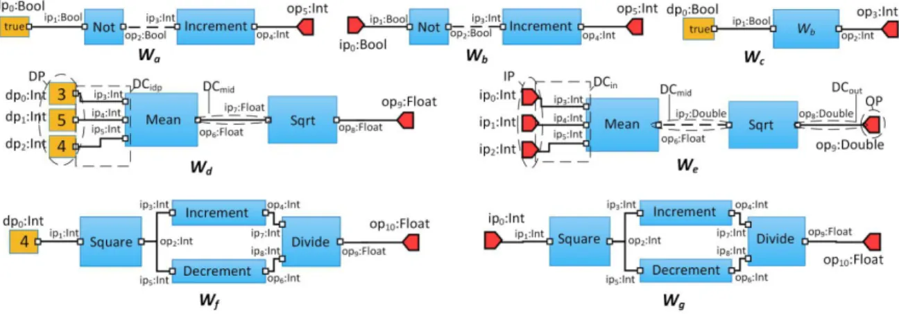
Figure 3.1: Examples of scientic workows (Wa, Wb, ..., Wg).
9. DCidp: DP →W*.IP is an inverse-functional one-to-many mapping. DCidpis a set of ordered pairs:
DCidp⊆{(dpi, ipk)|dpi∈DP, ipk∈Wj.IP, Wj∈W* }. That is, each pair in DCidprepresents a data channel that connects a data product dpi ∈ DP to the input port dpi ∈ DP of some component Wj ∈ W*.
To enhance readability, we provide a visual reference in Fig. 3.1. The gure shows seven representative workows that we will refer to in this paper as Wa, Wb, Wc, Wd, We, Wf, and Wg, respectively. These seven workows use other workows as their building blocks. Such constituent workows are shown as blue boxes with their ids written inside each box. Ports appear as red pins pointing right (input) or left (output). Data products are shown as yellow boxes with their values placed inside (e.g., true in Wa in Fig. 3.1). Because the order of input arguments of a workow matters (e.g., Divide workow in Wfin Fig. 3.1), we use ordered set IP to store a list of input ports. The term data channel refers to a wire, connecting a workow port to a data product or to another port. All entities from the set DCin ∪ DCmid ∪DCout ∪DCidp are data channels.
Each workow can be represented as a lambda expression. To simplify lambda expressions, we focus on workows with a single output port. We are currently extending our approach to allow set OP with a cardinality greater than one. Our denition requires that every workow and every data product has a unique id. For simplicity we also require that for any workow W, all ports of W and all ports of all workows in W* have unique ids.
We model workow Wd in Fig. 3.1 as a 9-tuple, where id = Wd, IP = ∅, OP ={(op9, Float)}, W* = {Mean, Sqrt}, DP = {(dp0, 3, Int), (dp1, 5, Int), (dp2, 4, Int)}, DCin =∅, DCout = {((Sqrt, op8), op9)}, DCmid = {((Mean, op6), (Sqrt, ip7))}, DCidp = {(dp0, (Mean, ip3)), (dp1, (Mean, ip4)), (dp2, (Mean, ip5))}. Workow We, on the other hand does not have concrete input data products connected to its inputs. We model it using 9-tuple with id = We, IP = {(ip0, Int), (ip1, Int), (ip2, Int)}, OP = {(op9, Double)}, W* = {Mean, Sqrt}, DP =∅, DCin = {( ip0, (Mean, ip3)), (ip1, (Mean, ip4)), (ip2, (Mean, ip5))}, DCout = {((Sqrt, op8), op9)}, DCmid = {((Mean, op6), (Sqrt, ip7))}, DCidp =∅.
Denition 3.1.4 (Primitive workow). A workow W is primitive if and only if it has both input and output ports, and W has neither constituent components, nor data products, nor data channels. Formally, W is primitive i
W.IP 6=∅ ∧ W.OP 6=∅ ∧ W.W* = W.DP = W.DCin = W.DCout = W.DCmid= W.DCidp
=∅.
We use isPrimitiveWF(W) to denote the above predicate.
Intuitively, primitive workow is a black box with inputs and outputs and that represents an atomic component (e.g., a Web service). Workows such as WS1, WS2, Not, Increment, Decrement, Sqrt, Square, Mean, and Divide in Fig. 3.1 and Fig. 4.1 are primitive.
Denition 3.1.5 (Composite workow). A workow W is composite if and only if it contains at least one reusable component (i.e. W.W* 6=∅) connected to ports and/or data products. Formally,
W is composite i
(W.W* 6= ∅ ∧ W.IP 6=∅ ∧ W.OP 6=∅ ∧ W.DCin 6=∅ ∧ W.DCout 6=∅) ∨ (W.W* 6=∅ ∧
W.OP 6=∅ ∧W.DP 6=∅ ∧W.DCidp 6=∅ ∧W.DCout 6=∅)
We use isComposite(W) to denote the above predicate. All workows in Fig. 3.1 and Fig. 4.1 are composite.
Intuitively, reusable workows are primitive or composite tasks that can be reused as building blocks of more complex workows. They are not executable as at least some of their input ports are not bound. Workows Wb, We and Wg in Fig. 3.1 are reusable. Workow Wb is reused inside Wc. Executable workows, on the other hand have all input data needed to perform computation. Workows Ws, Wa, Wc, Wd, and Wf in Fig. 4.1 and Fig. 3.1 are executable. Each executable
workow must contain at least one component and one data product connected to it. Thus, every executable workow is composite. The opposite is not true, as composite workow may be reusable (e.g., Wb), i.e. have input port(s) instead of concrete data product(s).
The above scientic workow model is serialized using a Scientic Worfklow Language. The XML schema of the latest version of the Scientic Worfklow Language (SWL 2.0) is shown in Appendix C. For example, the complete SWL specication of the workow Wa discussed earlier (Fig. 3.1) is shown in Fig. 3.2.
<workflowSpec> <workflow name="NotIncrement"> <workflowBody mode="graph-based"> <workflowGraph> <workflowInstances> <workflowInstance id="NOT15"> <workflow> NOT</workflow> </workflowInstance> <workflowInstance id="Increment19"> <workflow> Increment</workflow> </workflowInstance> </workflowInstances> <dataChannels>
<dataChannel from="NOT15.o1" to="Increment19.i1"/> </dataChannels>
</workflowGraph> <dataProductsToPorts>
<inputDP2PortMapping from="true" to="NOT15.i1"/> <outputDP2PortMapping from="Increment19.o1" to="outputDP0"/> </dataProductsToPorts> </workflowBody> </workflow> </workflowSpec>
Figure 3.2: The SWL specication of the workow Wa.
3.2 Workow Expressions
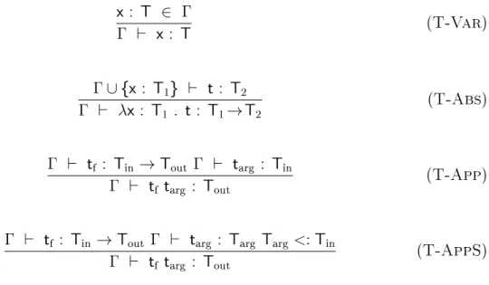
We rely on simply typed lambda calculus [66] enriched with a set of primitive types as a formal framework to reason about the behavior of workows. For example, expression λx:Int. Increment x is a function, or abstraction, that takes one integer argument, and returns its value
increased by 1. x is the abstraction name and Increment x is the expression of this abstraction. The expression Increment 3 is an application, which evaluates to 4.
Denition 3.2.1 (Workow expression). Given a workow W, its expression expr is a lambda expression that represents computation performed by W. If W is reusable, expr is an abstraction. If W is executable, expr is an application.
We now present our translateWorkow function outlined in Algorithm 1, that given a work-ow W, translates it into an equivalent lambda expression which performs the same computations and produces the same result as W.
We assume that workow diagrams are drawn horizontally with data owing from left to right (see Fig. 4.1, 3.1). Given a workow W, our translateWorkow algorithm translates com-ponents in W into lambda functions, and builds an expression whose structure corresponds to composition of components in W. Each connection between two components becomes a lambda application.
We accomodate workows nested inside each other to arbitrary degree via recursive calls to translateWorkow function that translates all sub-workows at each level of nesting (depth-wise translation). We translate arbitrary workow compositions within the same level of nesting (at compositions) by recursively calling the getInputExpression function outlined in Algorithm 2, that iterates over and translates all the connected components by backtracking along the data channels from right to left (breadth-wise translation).
Thus, our two algorithms together cover the full range of possible workow structures. We now provide a walk-through example by translating of Wd into an equivalent lambda expression. Example 3.2.2 (Translating workow Wd into an equivalent lambda expression).
Consider a workow Wd in Fig. 3.1. When the function translateWorkow(Wd) is called, it rst checks whether Wd is primitive, and because it is not, the else clause is executed (lines 5-34). translateWorkow rst determines that the component producing nal result of the entire workow Wd is Sqrt and stores it in the componentProducingFinalRes variable (line 14). Next, because Sqrt has a single input, for loop in lines 19-21 executes once, calling the function getInputExpression(Wd, Sqrt, ip7), whose output (Mean dp0 dp1 dp2) is stored into a string listOfArguments. Next, translateWorkow checks whether Wd is reusable (line 22), and because it is not, it returns the
application of workow expression for the Sqrt component to the list of arguments obtained earlier (line 32). Since Sqrt is a primitive workow, translateWorkow(Sqrt) returns its name Sqrt. Thus, the nal result of the translation is Sqrt (Mean dp0 dp1 dp2).
Example 3.2.3 (lambda expressions for workows Ws, Wa, Wb,..., Wg). We pro-vide lambda expressions obtained by calling our translateWorkow algorithm on each workow in Fig. 4.1, 3.1:
Ws : WS2 (WS1 dp0) Wa : Increment (Not dp0)
Wb : λx0:Bool. Increment (Not x0)
Wd : Sqrt (Mean dp0 dp1 dp2)
We : λx0:Int. λx1:Int. λx2:Int. (Sqrt (Mean x0 x1 x2))
Wf : Divide (Increment (Square dp0)) (Decrement (Square dp0)) Wg : λx0:Int. Divide (Increment (Square x0)) (Decrement (Square x0))
Note that executable workows (Ws, Wa, Wc, Wd, Wf) are translated into lambda appli-cations, whereas reusable ones (Wb, We, Wg) into lambda abstractions. Ports are translated into variables, e.g., port ip0appears as x0in the corresponding expression. We require that the workow expression is at, i.e. constituent componentsâ id's are replaced with their translations (see expression for Wc). Thus, a workow expression only contains port variables, names of primitive workows, and data products.
3.3 Type System for Scientic Workows
For interoperability, we adopt the type system dened in the XML Schema language spec-ication [101]. This allows us to mediate WSDL-based Web services since their input and output types are described in WSDL documents according to the XSD format. While our approach can accommodate all types dened in [101], in this paper we focus on the set of types that are most relevant to the scientic workow domain.
T ::= TPRIM | TXSD | T→ T
TPRIM ::= String |Decimal |Integer | NonPositiveInteger| NegativeInteger |NonNegativeInteger | UnsignedLong| UnsignedInt| UnsignedShort | |UnsignedByte| Double |PositiveInteger |Float |Long |Int |Short | Byte |Bool
TXSD ::= { e : TPRIM } | { e : TXSDii = 1 ... n }
In our approach we allow primitive types (TPRIM), XSD types (TXSD), and arrow types (T → T ). A primitive type, such as Int or Boolean describes an atomic value. An XSD Type consists
of an element name e and either a primitive type or an ordered set of other XSD types.
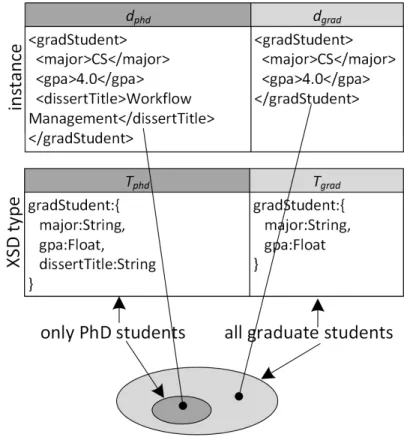
Example 3.3.1 (XSD Type). Consider an XML document dphd shown in Fig. 3.3 (top left)3 . We denote its XSD type as Tphd, consisting of a name gradStudent and an ordered set of three
3Although the two documents in Fig. 3.3 do not come from the scientic workow domain, we use them
children, each of which is another XSD type: {major:String}, {gpa:Float}, and {dissertTitle:String}, (see Fig. 3.3). The rst child has a name major and a type String.
Figure 3.3: Two sample XSD types.
In this work, we adhere to such notation for describing XSD types due to its conciseness compared to traditional XML Schema syntax. To improve readability, when discussing nested XSD types we omit curly braces at some levels of nesting. For simplicity, we focus on XML elements and do not explicitly model attributes. Since in XML each attribute belongs to a parent element, it can be viewed as a special case of an element without children.
The type constructor → is right-associative, i.e. the expression T1→T2→T3 is equivalent
with T1→(T2→T3). This type constructor is useful in dening types of reusable workows. For example, the workow Wbis of type Bool→Int, since it expects boolean value as input and produces an integer value as output. Workow W3 has the type Int→Int→Int →Double. The type of an executable workow is simply the type of its output, e.g., type of Wa is Int.
We have incorporated the proposed type system in the Data Product Language (DPL 2.0), which we use to serialize data product in the XML format. The XML schema of DPL 2.0 is shown in Appendix D.
3.4 Subtyping in Scientic Workows
We now introduce the notion of subtyping which is based on the fact that some types describe larger sets of values than others. For example, while the type Int describes whole numbers in the range [-2,147,483,648, 2,147,483,647], the type Decimal describes innite set of whole numbers multiplied by non-positive power of ten [101]. Thus, the set of values associated with the type Int is a subset of values associated with the type Decimal, or, in other words, the type Decimal describes larger set of values than Int does. Therefore, it is safe to pass an Int argument to a workow expecting a Decimal value as input.
Intuitively, given two types S and T, S is a subtype of T (denoted S <:T ), if all values of type S form a subset of values of type T. For the reader's convenience, Table 3.1 summarizes type denitions for the primitive types, as dened in the XML Schema language specication [101]. We use Z to denote a set of all integers, i.e., {..., -2, -1, 0, 1, 2, ...}, a commonly accepted notation.
While [101] includes positive and negative innity in value spaces of Double and Float, we omit them in our type system since they are not encountered in practical workow executions. We also leave out special cases such as not-a-number (NaN) values.
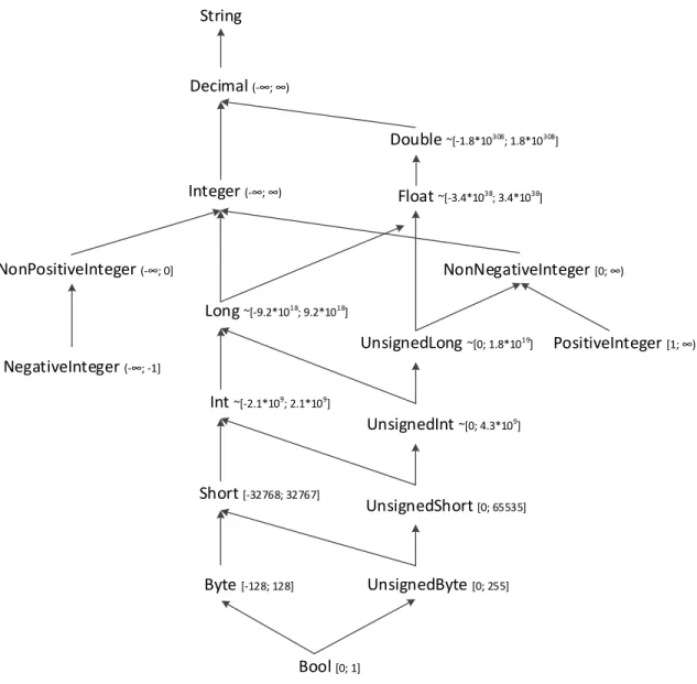
Based on the type denitions adopted from [101] summarized here in Table 3.1, we dene a set of inference rules specifying subtype relationships between primitive types. For example, it is easy to see from Table 3.1, that the set of Byte values is a subset of Short values, yielding a rule Byte <: Short. Fig. 3.4 shows a directed acyclic graph (DAG) that visualizes the subtype relationships (edges) between primitive types (nodes). A type S is a subtype of T if and only if there is a path from the node S to the node T. Thus, each edge in the subtyping DAG represent a subtyping inference rule.
Similar intuition about subtyping applies to the structured types, such as XSD types. All the documents of the type {a:Int} form a subset of documents associated with the type {a:Decimal}. Consider the two two XML documents shown in Fig. 3.3. The type Tphd describes a set of XML documents with the root element gradStudent that has at least three children named major, gpa and dissertTitle of types String, Float and String respectively. Type Tgrad on the other hand is less demanding as it requires only two child elements (major and gpa). Because Tphd is more specic, documents described by it form a subset of documents described by Tgrad, as shown in Fig. 3.3.
Table 3.1: A summary of primitive data types, adopted from [101].
Data type Denition Range
String set of nite-length sequences of characters N/A
Decimal {a |a = i ×10−n, i ∈Z, n ∈Z, and n ≥0} (-∞; +∞) Integer Z (-∞; +∞) NonPositiveInteger {a |a ∈Z, and a ≤0} (-∞; 0] NegativeInteger {a |a ∈Z, and a <0} (-∞; 0) NonNegativeInteger {a |a ∈Z, and a ≥0} [0;∞) PositiveInteger {a |a ∈Z, and a >0} (0; ∞) UnsignedLong {a | a∈Z, and a ≥0, and a ≤18446744073709551615} [0; 18446744073709551615]
UnsignedInt {a |a ∈Z, and a≥0, and a ≤4294967295} [0; 4294967295]
UnsignedShort {a | a∈Z, and a ≥0, and a ≤65535} [0; 65535]
UnsignedByte {a |a ∈Z, and a ≥0, and a ≤255} [0; 255]
Double {a = m ×2 e, m ∈Z,|m|<253, e ∈Z, and e ∈[-1075; 970]} ≈[-1.798 ×10308; 1.798×10308] Float {a = m ×2 e, m ∈Z,|m|<224, e ∈Z, and e ∈[-149; 104]} ≈[-3.402 ×1038; 3.402×1038] Long {a |a ∈Z, and a ≥-9223372036854775808, and a ≤9223372036854775807} [-9223372036854775808; 9223372036854775807] Int {a ∈Z, and a ≥-2147483648, and a ≤2147483647} [-2147483648; 2147483647]
Short {a ∈Z, and a ≥-32768, and a ≤32767} [-32768, 32767]
Byte {a ∈Z, and a ≥-128, and a ≤127} [-128, 127]
Bool {true, false} [0; 1]
Thus, it is safe to pass an argument of type Tphd to a workow expecting an input of type Tgrad since it will contain all the data needed by this workow plus some extra, which can be ignored.
More generally, an XSD type S is a subtype of another XSD type T (denoted S <: T ), if S's children form a superset of T 's children. Besides, if for each pair of corresponding children of S and T cs and ct, cs <: ct is true, then S <: T still holds. For example, if Tgrad.gpa was of type Decimal, Tphd<:Tgrad would still be true since Float <:Decimal.
String Decimal (- ; ) Integer (- ; ) NonPositiveInteger (- ; 0] NegativeInteger (- ; -1] NonNegativeInteger [0; ) UnsignedLong ~[0; 1.8*1019] PositiveInteger [1; ) UnsignedInt ~[0; 4.3*109] Double ~[-1.8*10308; 1.8*10308] UnsignedShort [0; 65535] UnsignedByte [0; 255] Float ~[-3.4*1038; 3.4*1038] Long ~[-9.2*1018; 9.2*1018] Int ~[-2.1*109; 2.1*109] Short [-32768; 32767] Byte [-128; 128] Bool [0; 1]
Figure 3.4: The subtyping DAG.
Such view of subtyping, based on the subset semantics, is called the principle of safe substi-tution. Workows Ws, Wa, Wb, and We in Fig. 3.1 and Fig. 4.1 are composed by this principle.
We formalize the subtype relation as a set of inference rules used to derive statements of the form S<:T, pronounced S is a subtype of T , or T is a supertype of S, or T subsumes S, where S and T are two types.
As shown in Fig. 3.5, the rst two rules (S-Refl and S-Trans) state that the subtype relation is reexive and transitive.
They are then followed by a set of rules for primitive data types (collectively labeled S-Prim) derived from the hierarchy presented in [101]. As Bool type is less descriptive than Byte (true and
T<:T (S-Refl) S<:U U<:T S<:T (S-Trans) Decimal<:String Integer <:Decimal NonPositiveInteger<:Integer NegativeInteger<:NonPositiveInteger Long <:Integer Int<:Long Short<:Int Byte<:Short Bool<:Byte Double<:Decimal Float<:Double
Long<:Float (S-Prim)
UnsignedInt<:Long UnsignedShort<:Int UnsignedByte<:Short Bool<:UnsignedByte NonNegativeInteger <:Integer UnsignedLong <:NonNegativeInteger UnsignedInt<:UnsignedLong UnsignedShort<:UnsignedInt UnsignedByte<:UnsignedShort UnsignedLong<:Float PositiveInteger<:NonNegativeInteger {Sii∈1...n}⊆{Ujj∈1...n+k}, n≥1, k≥0, for each i ∈ 1...n Si<:Ti {e:Ujj∈1...n+k}<:{e:Tii∈1...n} (S-XSD)
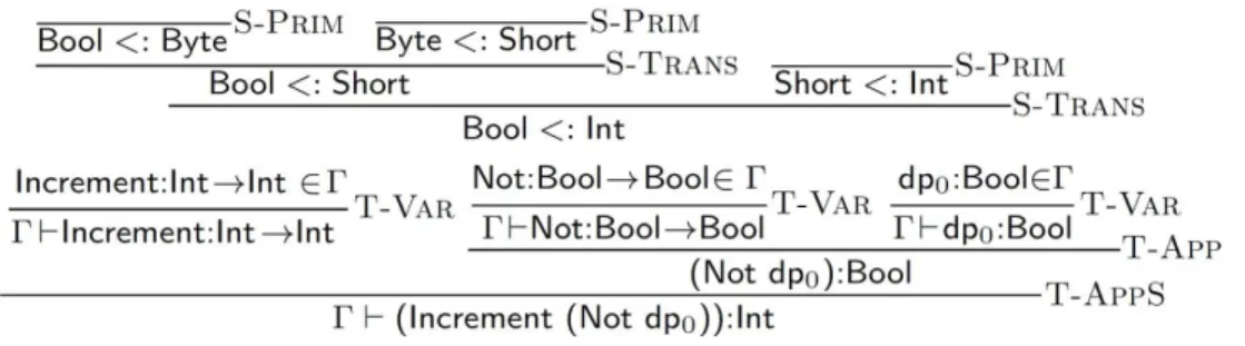
false can be mapped to 1 and 0, a subset of Byte), we consider Bool to be a subtype of Byte. The range of Long values is [-9,223,372,036,854,775,808, 9,223,372,036,854,775,807], which is a superset of Int values discussed above, hence Int<:Long. We also include a rule S-XSD that formalizes the intuitive notion of subtyping for XSD types. This rule can be used, for example to infer that the type Tphd <:Tgrad (Fig. 3.3).
Denition 3.4.1 (Subtype relation). A subtype relation is a binary relation between types, S <:T that satises all instances of the inference rules in Fig. 3.5.
Thus, according to the Denition 3.4.1, the existence of the subtyping derivation concluding that S <: T shows that S and T belong to the subtype relation. We now show the use of the inference rules in Fig. 3.5 to infer subtyping.
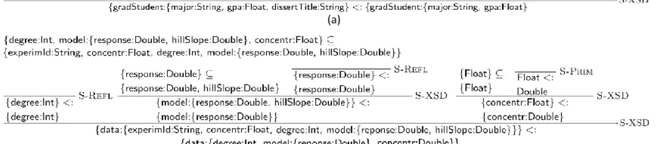
Example 3.4.2 (Subtyping derivation inferring Tphd <:Tgrad). Fig. 3.6(a) shows subtyping derivations concluding that the two types Tphdand Tgradin Fig. 3.3 belong to the subtype relation, i.e. Tphd<:Tgrad.
(a)
(b)
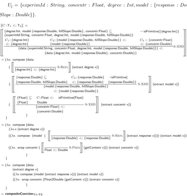
Figure 3.6: Sample subtyping derivations. (a) Tphd <: Tgrad. (b) T1 <: T2 from Ws.
Each derivation step is labeled with the corresponding subtyping inference rule. In Fig. 3.6(a) we rst note that the set {major:String, gpa:Float} is a subset of {major:String, gpa:Float, dissert-Title:String}. We then show that {major:String} is a subtype of {major:String} using S-Refl rule. Similarly we show that {gpa:Float} is a subtype of {gpa:Float}. These three statements together form a premise from which we can infer that {gradStudent: {major:String, gpa: Float, dissertTi-tle: String}} <: {gradStudent: {major:String, gpa:Float}} based on the rule S-XSD as shown in Fig. 3.6(a). This derivation formalizes the intuition that if a workow can handle XML documents describing graduate students it can certainly handle documents describing PhD students.
Example 3.4.3 (Subtyping derivation inferring T1 <: T2). Fig. 3.6(b) shows a subtyping derivation inferring that the two types T1and T2in Fig. 4.1 belong to the subtype relation, i.e. T1 <:T2. As shown in the gure, here we use four statements to form a premise from which we derive that T1 <:T2according to the rule S-XSD.
In practice, the need arises to algorithmically determine whether for the two given types S and T the statement S<:T is true. To this end, we now present a function that given two types S and T returns true if S<:T and false otherwise. The function subtype is outlined in Algorithm 3.
An XSD type T is a data structure containing element name e and an ordered set of children T.children. If|T.children |>1, then each element in T.children is another XSD type. If|T.children |= 1, then a single child (T.children[0]) is either a primitive type or an XSD type. We assume the
existence of several functions that are described as follows. The function isPrimitive(T) returns true if T is a primitive type and false otherwise. The function isXSDType(T ) checks whether a given type is an XSD type. The function ndChildWithTheName(name, E) returns an item c from the set of XSD types E such that c.e = name. Finally, the function subtypePrim(S, T ) embodies rules S-Refl, S-Trans, and S-Prim by returning true if two given primitive types belong to the subtype relationship. For example, subtypePrim(Int, Float) returns true, whereas subtypePrim(Float, Int) returns false. As all four of these functions are trivial we omit their details for brevity.
Example 3.4.4 (Determining that Tphd <: Tgrad using the subtype function). When the function subtype(Tphd, Tgrad) is invoked, it rst checks whether the two types are equal (line 4), and since Tphd 6= Tgrad it proceeds to line 5 to check whether both types are primitive. Since both Tphdand Tgrad are XSD types (i.e. not primitive) the algorithm enters the else if clause (lines 7-28). It rst ensures that both element names are the same (gradStudent) (line 8). It then checks whether Tphd and Tgrad are both simple types, i.e. they do not contain nested XSD types inside (lines 9-11). Since bothTphdand Tgrad are complex types, the algorithm builds two sets of element names of children of both types (lines 16-22):
childrenNamesOfS = {major, gpa, dissertTopic} childrenNamesOfT = {major, gpa}
It then checks whether the set childrenNamesOfT is a subset of childrenNamesOfS (line 19) and because it is, the algorithm iterates over every child in T.children, nds corresponding child from S.children (i.e. child with the same element name) and checks whether they belong to the subtype relation (lines 20-25). If at least one pair of correspondng children did not satisfy the subtype relation, the algorithm would return false. For example, if Tphd.gpa was Decimal, the algorithm would detect it and return false, since {gpa:Decimal} is not subtype of {gpa:Float} (lines 22-24). However, since every pair of respective children satises the subtype relation, after iterating over each pair the algorithm returns true (line 26). Note that the algorithm would still return true if for example Tgrad.gpa was of type Decimal since {gpa:Float} <:{gpa:Decimal}.

![Table 3.1: A summary of primitive data types, adopted from [101].](https://thumb-us.123doks.com/thumbv2/123dok_us/11059046.2992706/38.918.133.787.145.811/table-summary-primitive-data-types-adopted.webp)