from interval data
.
White Rose Research Online URL for this paper:
http://eprints.whiterose.ac.uk/147064/
Version: Accepted Version
Article:
Pudney, S. orcid.org/0000-0002-5697-0976 (Accepted: 2019) IntCount: a Stata command
for estimating count data models from interval data. The Stata Journal. ISSN 1536-867X
(In Press)
© 2019 StataCorp LLC. This is an author-produced version of a paper subsequently
published in The Stata Journal. Uploaded in accordance with the publisher's self-archiving
policy.
[email protected] https://eprints.whiterose.ac.uk/ Reuse
Items deposited in White Rose Research Online are protected by copyright, with all rights reserved unless indicated otherwise. They may be downloaded and/or printed for private study, or other acts as permitted by national copyright laws. The publisher or other rights holders may allow further reproduction and re-use of the full text version. This is indicated by the licence information on the White Rose Research Online record for the item.
Takedown
If you consider content in White Rose Research Online to be in breach of UK law, please notify us by
IntCount: a Stata command for estimating
count data models from interval data
Stephen Pudney
Health Economics and Decision Science School of Health and Related Research
University of Sheffield Sheffield, UK
Abstract. This article describes a user-written Stata command,intcount, for
estimation of a number of regression models for count data which are observed in interval form. The models available are Poisson, negative binomial and binomial, and they can be estimated in standard or zero-inflated form. Use of the command is illustrated with an application to analysis of data from the UKUnderstanding Society survey on the demand for healthcare services.
Keywords: st0001, count data, interval data, zero-inflated, interpolation, Under-standing Society
1
Introduction
Many survey variables are naturally non-negative integer-valued counts, for example the number of times an action or event has occurred within a given observation period. Count data regression models based on distributions such as the Poisson and negative binomial are widely used for the analysis of these variables.
But complications arise when survey questions are not designed to reveal the count exactly. Survey designers sometimes argue that questions may yield more reliable (albeit less detailed) data if they ask the respondent to place the count within one of a number of pre-specified intervals, rather than to report a specific figure.
Interval observation of count data causes difficulty in the estimation of count data regressions, since most available software requires the count to be observed exactly. There is therefore a need for estimation procedures which can take account of coarse interval observation.1
Another aspect of the problem is that many types of descriptive or policy analysis require exact rather than interval counts, so some form of imputation or interpolation is required.
This article describes a new Stata command for interval estimation of a number of count data models, and reports results from an illustrative application. Section 2 sets
1. A Stata commandintregalready exists for interval estimation of the regression model for a con-tinuous dependent variable such as income, sointcountserves to widen the range of models for which interval estimation is possible. Note however thatincounthas a much wider range of pre-diction/interpolation options thanintreg.
out the estimation approach and the range of available models; section 3 details the syntax of the estimation command and the linkedpredictcommand that can be used for various types of post-estimation imputation. Section 4 presents an application to healthcare data from the UKUnderstanding Society survey and section 5 concludes.
2
Interval-observed count data models
2.1
Basic setup
Let Yi ≥ 0 be the ith observation on a dependent variable which takes non-negative integer values. Yi may be bounded or unbounded. However, our observations are not on Yi itself but rather an interval within which Yi lies. Consequently, we have two observed dependent variables,[Li, Ui]with the property that:
Li≤Yi≤Ui (1)
The numerical values of the interval bounds[Li, Ui]vary across observations but they are assumed to be observed and strictly exogenous. The two bounds may be equal for some observations whereYi is fully observed and, for unbounded distributions like the Poisson and negative binomial, the upper boundUi may be infinite for some observa-tions.
A set of explanatory covariates appear in a vector Xi, and we assume a known parametric form for the discrete conditional probability functionf(.)and corresponding distribution function F(.), defined for any non-negative integery:
P r(Yi=y∣Xi) = f(y∣Xi) (2) P r(Yi≤y∣Xi) = F(y∣Xi) (3) The conditional probability of observing the eventLi≤Yi≤Ui is:
P r(Li≤Yi≤Ui∣Xi) = F(Ui∣Xi)−F(Li−1∣Xi)
= ∑Ui
y=Li
f(y∣Xi) (4)
where F(Li−1∣Xi)is understood to be zero forLi=0.
2.2
Alternative base distributions
The model is completed by a specifying a parameterized functional form for the dis-tribution function F(.∣Xi). The command offers nine possibilities, formed from three alternative base models and three options for zero-inflation. Leaving aside the possibility of zero-inflation, the available models for F(.∣Xi)are as follows:
Poisson:
f(y∣Xi)=e −λi
where λi is the conditional mean function E(Yi∣Xi), parameterised as eXiβ. The conditional mean and variance of the count variable are both equal toλi.
Binomial: f(y∣Xi) = ( Mi y )p y i(1−pi) Mi−y (6)
where Mi is the known maximum possible value, which may vary exogenously across observations, and pi is the binomial probability, parameterised as pi = [1−e−Xiβ]
−1
. The conditional mean function is E(Yi∣Xi) =Mipi. This specification may be appro-priate when there is a natural upper limit to survey responses (e.g. to the question ”on how many days last month did you use cannabis?”).
Negative binomial: is derivable as the following Poisson-gamma mixture: y∣ν∼Poisson(λiν); ν∼gamma(1
α, α) (7)
where λi = eXiβ
, α > 0. This gives a distribution for y with mean λi and variance 1+αλi. Note that, in the terminology of Cameron and Trivedi (2013)), this is the NB2 parameterization of the negative binomial regression model, and is consistent with the specification implemented in the Statazinbcommand. The ML estimation procedure treats lnαas an unrestricted constant parameter.
2.3
Zero-inflation
In some count data applications, standard forms like the binomial, Poisson and negative binomial are found to understate the frequency of zero counts. One way of dealing with this is to use a double hurdle or mixture process, where some individuals have a degenerate zero count with probability 1, while others have a count drawn from a standard distribution such as the Poisson.
Let the conditional probability of a degenerate zero be given by the following linear index model:
P r(degenerate 0∣Xi) =π(Xi1γ) (8)
where Xi1 is a subvector of Xi. The distribution of Y among the non-degenerate
population is g(y∣Xi2β), where Xi2 is another subvector of Xi. Then the mixture
distribution ofY is: f(y∣Xi) =⎧⎪⎪⎪⎨⎪⎪⎪ ⎩ π(Xi1γ) + (1−π(Xi1γ))g(0∣Xi2β) ify=0 (1−π(Xi1γ))g(y∣Xi2β) ify>0 (9)
The probability of the observed interval [Li, Ui]is again given by (4). Theintcountcommand offers three options for zero-inflation:
logit: π(Xi1γ) =[1+exp(−Xi1γ)]
−1
probit: π(Xi1γ)=Φ(Xi1γ)
In practice, estimates of the logit and probit variants are usually almost identical apart from scaling of the γ coefficients, which are larger by a factor of approximately π/√3.
2.4
Estimation
Estimation is by maximum likelihood (ML), with probabilities of the form (4) used to construct the log-likelihood function. By default, numerical optimization of the log-likelihood is carried out using Stata’s modified Newton-Raphson optimizer; other algorithms can be substituted in case of difficulty in obtaining convergence (see (Stat-aCorp 2017, pp. 639-686) for details). Optimization is based on thelf0evaluator, so log-likelihood derivatives are approximated by finite differences.
Experience to date suggests that this works very well in most cases. Difficulties are most likely to be encountered in connection with over-specified models involving zero-inflation which is not required by the data, in which case one or more parameters in the coefficient vectorγ will explode. Similar convergence difficulties may be found also in zero-inflated specifications where zero-inflation is required empirically for a group with certain values for the variablesXi2but not for other sample groups. Convergence
problems of these types are usually easy to spot and the required model re-specification obvious.
Occasionally (usually in the more heavily parameterized zero-inflated specifications), the optimizer reaches a difficult region with almost flat likelihood or discontinuous approximate derivatives. Often these problems can be resolved by passing down as starting values for the optimization the estimates from a simpler specification – for example a model without zero-inflation or with constant zero-inflation, or a Poisson model as a simpler alternative to the negative binomial.
2.5
Prediction and imputation
The estimates provided by intcount may often be useful for imputation, and the
predict command available with intcount offers a range of options. Particularly useful are: the interval-conditional mean predictorY∗
i = E(Yi∣Li ≤Yi ≤ Ui, Xi); and the interval-conditional random draw, Y+
i which is a realization of the distribution of Yi∣Li≤Yi≤Ui, Xi. Two common situations illustrate their use.
One is where we would like to use the unobserved variable Yi as a covariate in another model – for example a regression of some dependent variableWionYiandXi. ButYi is unobserved and we only know that it lies within an interval [Li, Ui]. Then
intcountcan be used to estimate a count data model for Yi onXi and compute the interval-conditional mean predictorY∗
i . The use ofY ∗
i as a proxy for Yi introduces an imputation error proportional to (Yi−Y∗
straightforward to show thatE{(Yi−Y∗ i )∣Y
∗
i , Xi} =0, so the residual is orthogonal to the constructed proxy forYi, and the regression of Wi on Yi, Xi therefore gives unbiased coefficients under standard classical assumptions (provided the count data model for Yi∣Xi is well specified). This is a better solution to the imputation problem than the common practice of using interval mid-points. However, it can be improved further by making random draws Y+
i and using single or multiple imputation.
2
Another common application is where exact values for Y are needed within some complex policy simulation. Again, multiple random drawsY+
i can be used in place of the unobservedYi, and the policy calculations averaged across replications. The healthcare cost analysis by Davillas and Pudney (2019) is an example of this.
3
Command syntax
3.1
intcount
intcount depvar1 depvar2 [indepvars] [if ] [in] [weight],
[ poisson | binomial(# | varname) | negbin
inflate(varlist | cons[,offset(varname)]) noconst probit [other options] ] Description
intcount is a user-written program which allows the estimation of a range of count data models in cases where some or all of the observations on the dependent variable are intervals containing the count, rather than the count itself. The models are based on Poisson, Binomial or Negative Binomial distributions, possibly with zero-inflation. It thus covers some of the same ground as existing Stata commandspoisson, nbreg,
binreg,zipandzinbreg, but allowing for interval-form data.
depvar1anddepvar2are variables that specify the upper and lower limitsLiandUiof the interval containing the unobserved true countYi. The covariatesXi1 for the core
Poisson, binomial or negative binomial model are specified inindepvars; an intercept will automatically be included unless thenoconstoption is used.
Output
intcountreturns maximum likelihood estimates of the parameters of a count data model, allowing for the possibility that some or all of the observations on the dependent variable have the form of an interval containing the count, rather than the count itself. Main options
noconstis used to suppress the intercept term in the linear indexXi1β
poissonspecifies the Poisson base model defined by equation (5).
2. See Manski and Tamer (2002) for a much fuller and more general discussion of inference from interval data.
binomial(#—varname) specifies the binomial model (6). If the count limit Mi is con-stant across observations, # gives that fixed positive number; otherwise varname
specifies a variable containingMi.
negbinspecifies the negative binomial model.
At most one of the three optionspoisson,binomial(varname) andnegbinmay appear. If all three are omitted,poissonis used as the default.
inflate(varlist[, noconst])specifies the variablesXi2used as covariates in the
zero-inflation model (if any). An intercept is included in the zero-zero-inflation model unless thenoconstmodifier is used. If inflateis omitted, zero-inflation is not used and a standard count data specification is estimated. If it appears as inflate( cons), the zero-inflation probability is estimated as a constant. If covariates are specified in varlist, an intercept will also be included unless the[, noconst] sub-option is used.
probitspecifies the zero-inflation model to be of probit form. If omitted, the default is logit. Theprobitoption may only be used ifinflatealso appears.
Other options
offset(varname)includes varnamein the model with coefficient constrained to 1
exposure(varname)includes ln(varname) in the model with coefficient fixed at 1 Standard options for controlling the ML optimization procedure can be included, most usefully:
from(matrixname), specifying the name of a single-row matrix containing user-supplied initial parameter values for the optimization. The column names should take the formmodel:variablenameandmodel: consfor the coefficients and intercept in the linear indexXiβ;inflate:variablenameandinflate: consfor those in the index Xi2γ of the zero-inflation mechanism. The column name for theln(α)parameter
of the negative binomial model should be given as/:lnalphaif running with Stata version 15, or lnalpha: cons for version 14 or earlier.3
The vector may contain irrelevant elements, since the vector is passed onto the ML optimizer with the , skipmodifier.
difficultmay very occasionally help overcome convergence difficulties
3.2
predict
predict outputvarname [if ] [in],[ predicttype ]
Description
3. This is for consistency withnbregandzinb– the column labelling of theln(α)parameter in the
return vectore(b)from thenbregandzinbchanged between Stata versions 14 and 15. If a starting value forln(α)is supplied with the wrong labelling, it will be ignored byintcount.
Followingintcount, the predict command can be used to construct several measures conditional on covariate values, including: the expected count; the probability of the count falling in a specified interval; and the expected value of the count, conditional on it lying in a specified interval. It is also possible to generate a random draw the interval-specific conditional count distribution. These predict options are particularly useful for interpolation purposes. The specified type of prediction is returned in outputvarname
as a double precision variable. Options and output
pr(#|var #|var)is the predicted probability (conditional on covariate values) that the count lies in the interval defined by lower and upper limits that may each be a fixed number or a variable.
ce(#|var #|var)is the expectation of the count conditional on the covariates and the event that it lies in the interval defined by the two limits which may be variable or constant.
mc(#|var #|var [, uniformvar]) generates a single random draw from the distribu-tion of y conditional on the event that it lies in the interval defined by the two specified limits. If the [,uniformvar] option is not used,intcountwill generate the required pseudo-random numbers itself, without resetting the random number seed. Optionally, the simulation can be controlled completely by passing a variable con-taining uniform pseudo-random numbers. The mcoption is useful for Monte Carlo simulation or imputation applications where distributional characteristics beyond the conditional mean are required.
n gives a prediction of the count conditional only on the covariates. If no predicttype
option is declared, this is the default.
nooffsetBy default, any offset or exposure adjustment used for estimation will also be incorporated in the predictions of typepr,ceorn; the optionnooffsetwill cause offset or exposure adjustments to be ignored.
4
An application to healthcare demand
We apply the intcount command to data from wave 7 of theUnderstanding Society
UK panel on the use of health care services. The questions distinguish three types of service: consultations with a general practitioner (GP), attendance at a hospital out-patient (OP) clinic, and hospital in-patient (IP) stays.4
The first two dependent variables come from the following survey questions:
“In the last 12 months, approximately how many times have you talked to, or visited a GP or family doctor about your own health? Please do not include any visits to a hospital.”
4. The data and a more comprehensive application are discussed in detail in Davillas and Pudney (2019).
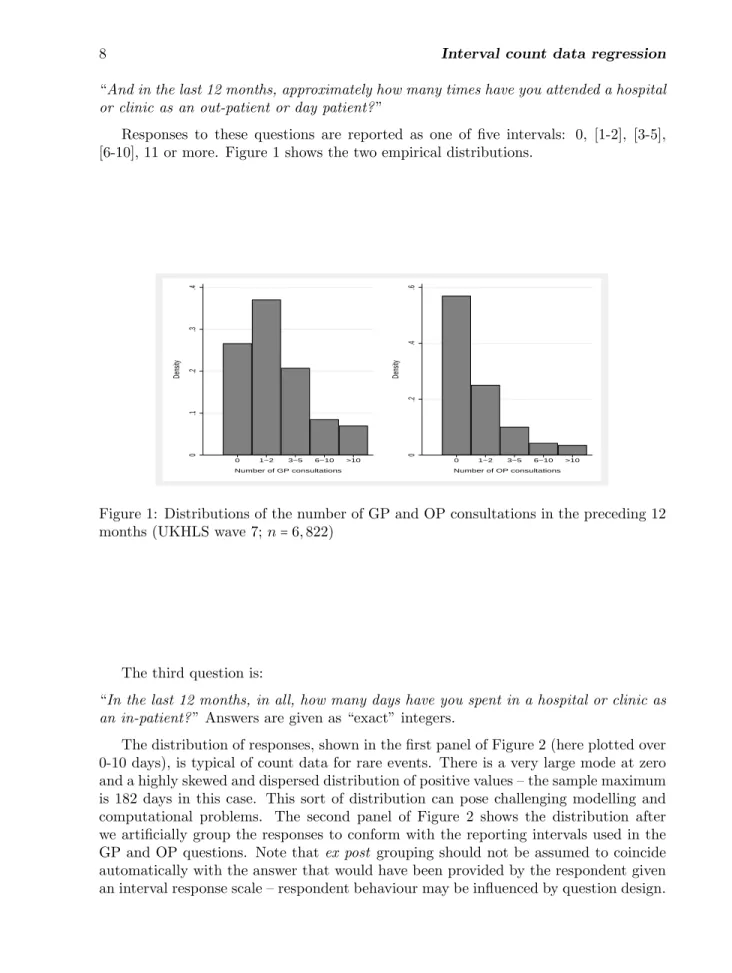
“And in the last 12 months, approximately how many times have you attended a hospital or clinic as an out-patient or day patient?”
Responses to these questions are reported as one of five intervals: 0, [1-2], [3-5], [6-10], 11 or more. Figure 1 shows the two empirical distributions.
0 .1 .2 .3 .4 Density 0 1−2 3−5 6−10 >10 Number of GP consultations 0 .2 .4 .6 Density 0 1−2 3−5 6−10 >10 Number of OP consultations
Figure 1: Distributions of the number of GP and OP consultations in the preceding 12 months (UKHLS wave 7;n=6,822)
The third question is:
“In the last 12 months, in all, how many days have you spent in a hospital or clinic as an in-patient?” Answers are given as “exact” integers.
The distribution of responses, shown in the first panel of Figure 2 (here plotted over 0-10 days), is typical of count data for rare events. There is a very large mode at zero and a highly skewed and dispersed distribution of positive values – the sample maximum is 182 days in this case. This sort of distribution can pose challenging modelling and computational problems. The second panel of Figure 2 shows the distribution after we artificially group the responses to conform with the reporting intervals used in the GP and OP questions. Note thatex post grouping should not be assumed to coincide automatically with the answer that would have been provided by the respondent given an interval response scale – respondent behaviour may be influenced by question design.
0 1 2 3 4 5 Density 0 2 4 6 8 10 Number of IP days 0 .2 .4 .6 .8 1 Density 0 1−2 3−5 6−10 >10 Number of IP days
Figure 2: Distribution of the number of days as hospital inpatient in the preceding 12 months, as observed and after grouping (UKHLS wave 7;n=6,824)
4.1
Hospital in-patient days: the effect of grouping
First consider the choice of distributional form, using the original exact data. The
intcountcommand can accommodate exact count data by setting the upper and lower limit variables equal to the exact count. The resulting estimates reproduce exactly those produced bypoissonorzipfor the Poisson model,binregfor the binomial model5
, and
nbregorzinbfor the negative binomial model. The covariates used in these models are simple demographics: a cubic in agea(measured in decades from an origin of 50 years), membership of any ethnic minoritynonw, an indicator for the absence of any educational qualificationnoed and another for degree-level education degree. The following code produced alternative gender-specific models, whose sample fit is summarised in Table 1 using the Akaike (AIC) and Bayesian (BIC) information criteria.
. global Xvars "a a2 a3 nonw noed degree" . // No zero-inflation
. forvalues i=0/1 {
2. intcount IP IP $Xvars if male== `i´, poisson vce(robust) 3. estat ic
. intcount IP IP $Xvars if male== `i´, binomial(365) vce(robust) 4. estat ic
. intcount IP IP $Xvars if male== `i´, negbin vce(robust) 5. estat ic
6. }
. // With zero-inflation . forvalues i=0/1 {
2. intcount IP IP $Xvars if male== `i´, inflate($Xvars) poisson vce(robust) 3. estat ic
. intcount IP IP $Xvars if male== `i´, inflate($Xvars) binomial(365) vce(robust) 4. estat ic
. intcount IP IP $Xvars if male== `i´, inflate($Xvars) negbin vce(robust) 5. estat ic
5. There appears to be no available Stata command for estimating the zero-inflated binomial model, andintcountnow fills that gap.
6. }
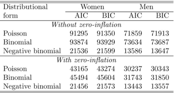
It is clear from Table 1 that the negative binomial model is far superior in terms of sample fit to the Poisson and binomial models, and also that zero-inflation improves the fit substantially.
Table 1: Akaike and Bayesian information criteria for zero-inflated versions of Poisson, binomial and negative binomial count data models, estimated separately by gender from exact data on days spent in hospital.
Distributional Women Men
form AIC BIC AIC BIC
Without zero-inflation Poisson 91295 91350 71859 71913 Binomial 93874 93929 73634 73687 Negative binomial 21536 21599 13586 13647 With zero-inflation Poisson 43165 43274 30237 30343 Binomial 45494 45604 31743 31850 Negative binomial 21456 21573 13443 13557
We now investigate the effect of data grouping by re-estimating the model using the artificially grouped form of the variable whose distribution is shown in Figure 2. The code is as follows:
. forvalues i=0/1 {
2. intcount IP IP $Xvars1 if male== `i´, inflate($Xvars1) negbin vce(robust) 3. estimates store exact`i´
4. intcount lo_IP hi_IP $Xvars1 if male== `i´, inflate($Xvars1) negbin vce(robust) 5. estimates store grouped`i´
6. }
. estout exact0 grouped0 exact1 grouped1, cells(b(star fmt(%7.3f)) /// > se(par)) starlevels(* .1 ** .05 *** .01) style(tex)
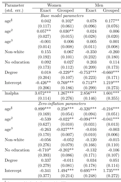
Table 2 compares the parameter estimates. There are substantial parameter differ-ences, particularly for the age and education effects in the female sample.
Table 2: Estimates of zero-inflated negative binomial model estimated from exact and artificially grouped data.
Parameter Women Men
(std. err.) Exact Grouped Exact Grouped
Base model parameters
age§ 0.042 0.102* 0.078 0.177** (0.117) (0.061) (0.096) (0.076) age2 0.057** 0.030** 0.024 0.006 (0.027) (0.015) (0.028) (0.020) age3 -0.001 0.006 0.005 0.001 (0.014) (0.008) (0.011) (0.008) Non-white 0.155 0.067 -0.350 -0.260 (0.192) (0.101) (0.232) (0.180) No education 0.092 0.027 0.203 0.114 (0.173) (0.112) (0.209) (0.173) Degree 0.018 -0.229** -0.753*** -0.660*** (0.204) (0.107) (0.223) (0.171) Intercept -0.426** 0.769*** 0.713** 1.219*** (0.206) (0.186) (0.299) (0.273) lnalpha 3.072*** 1.267*** 2.856*** 1.601*** (0.114) (0.276) (0.146) (0.355) Zero-inflation parameters age§ 0.899*** 0.258*** -0.320*** -0.216*** (0.169) (0.054) (0.094) (0.051) age2 -0.539 -0.022** -0.094*** -0.041*** (0.627) (0.010) (0.031) (0.013) age3 -0.263 -0.027*** -0.016 -0.003 (0.170) (0.007) (0.010) (0.006) Non-white -0.056 -0.052 -0.120 -0.015 (0.276) (0.079) (0.166) (0.110) No education -0.710* -0.202** -0.132 -0.106 (0.393) (0.086) (0.171) (0.107) Degree 0.337 -0.011 0.034 0.051 (0.279) (0.081) (0.178) (0.114) Intercept -0.341 1.494*** 0.695*** 1.735*** (0.377) (0.214) (0.248) (0.272)
§Age measured in decades from an origin of 50. Statistical significance: * = 10%, ** = 5%, *** = 1%
Figure 3 shows the implications of parameter differences for the estimated age pro-files, plotting the probability of hospitalizationP r(y >0∣age)againstagein the range 16-85, with other covariates set to modal zero values. The relevant code is as follows:
. preserve . replace age=.
(42,210 real changes made, 42,210 to missing) . replace age=_n+15 if _n<=70
(70 real changes made) . replace a=(age-50)/10
(42,210 real changes made, 42,140 to missing) . replace a2=a^2
(42,209 real changes made, 42,140 to missing) . replace a3=a*a2
(42,210 real changes made, 42,140 to missing) . replace nonw=0
(30,402 real changes made) . replace noed=0
(14,694 real changes made) . replace degree=0
(18,067 real changes made) . gen ll=0 if age<.
(42,147 missing values generated) . gen uu=0 if age<.
(42,147 missing values generated) . forvalues i=0/1 {
2. foreach d in exact grouped { 3. estimates restore `d´`i´
4. predict p`d´`i´ if age<=85,pr(1 .) 5. }
6. }
(results exact0 are active now) (results grouped0 are active now) (results exact1 are active now) (results grouped1 are active now) . sort age
. twoway line pexact0 pgrouped0 age if age<=85 , lpattern(solid dash) /// > graphregion(fcolor(white) ilcolor(white) icolor(white) lcolor(white) ) /// > lcolor(black) name(p0, replace) xlabel(20(10)80) ylabel(0(0.05)0.2) /// > xscale(titlegap(3)) yscale(titlegap(3)) xtitle("Woman´s age") /// > legend(col(1) pos(5) ring(0) label(1 "exact") ///
> label(2 "grouped")) ytitle("Pr(hospitalization)")
. twoway line pexact0 pgrouped0 age if age<=85 , lpattern(solid dash) /// > graphregion(fcolor(white) ilcolor(white) icolor(white) lcolor(white) ) /// > lcolor(black) name(p1, replace) xlabel(20(10)80) ylabel(0(0.05)0.2) /// > xscale(titlegap(3)) yscale(titlegap(3)) xtitle("Man´s age") ///
> legend(col(1) pos(5) ring(0)label(1 "exact") /// > label(2 "grouped")) ytitle("Pr(hospitalization)") . graph combine p0 p1
The estimated age profiles remain broadly similar after grouping but they display more variability for the estimates based on exact data, so coarsening the counts to interval form has a mild smoothing effect in this example.
0 .05 .1 .15 .2 Pr(hospitalization) 20 30 40 50 60 70 80 Woman’s age exact grouped 0 .05 .1 .15 .2 Pr(hospitalization) 20 30 40 50 60 70 80 Man’s age exact grouped
Figure 3: Predicted age profile of zero count probability by age for ethnic majority woman and man with mid-level education
It is also striking in this application that grouping has a perverse effect on the standard errors. It is clear theoretically that recoding count data to coarser interval form must reduce statistical precision of the parameter estimator for a well-specified count data model (this is easily confirmed empirically using Monte Carlo simulation by applying intcountto simulated counts in exact and grouped form). However, the anticipated loss of precision may not occur for computed standard errors when the count data model is misspecified. A poor model may do quite well in fitting the distribution of responses within broad intervals, but much worse in fitting the distribution of exact counts within those intervals. Parameter estimates may be (asymptotically) biased in different ways for grouped and exact data, and the computed confidence intervals (which are not statistically valid for misspecified models) need not be wider for the interval estimates. This is what we find in Table 2, where the interval estimates have robust standard errors that are always smaller, very much so in many cases.
4.2
Interpolated healthcare measures
Theintcountcommand has been designed to be usable as a basis for interpolation of the underlying count from coarse interval data. We now turn attention to the GP and OP variables, again taking the negative binomial as our basic model, but considering both standard and zero-inflated (probit) variants. As covariates, we use dummy variables to allow for gender and ethnicity effects, a cubic in age, and a 4-level categorization of educational attainment. Table 3 gives results and also includes estimates of the logit variant for the OP data. Comparison of the fourth and fifth columns of Table 3 confirms that the choice between probit and logit specifications makes virtually no difference to the estimates, except for scaling of the zero-inflation coefficients (which are larger for the logit model by approximately√π2/3=1.814).
Table 3: Estimates of negative binomial models for counts of GP and hospital OP consultations, estimated from grouped data.
GP consultations Hospital OP consultations Parameter no zero Probit no zero Probit Logit (std. err.) inflation inflation inflation inflation inflation
Base model parameters
age§ 0.094*** 0.068*** 0.168*** 0.065*** 0.064*** (0.009) (0.009) (0.014) (0.016) (0.016) age2 0.001 0.001 0.006* 0.003 0.003 (0.002) (0.002) (0.003) (0.004) (0.004) age3 0.001 0.002** 0.001 0.006*** 0.007*** (0.001) (0.001) (0.002) (0.002) (0.002) Male -0.368*** -0.280*** -0.321*** -0.137*** -0.139*** (0.015) (0.016) (0.023) (0.027) (0.027) Minority -0.139*** -0.130*** 0.046* 0.012 0.016 (0.017) (0.018) (0.027) (0.031) (0.031) GCSE -0.148*** -0.147*** -0.052 -0.085** -0.084** (0.021) (0.021) (0.033) (0.035) (0.035) A-level -0.268*** -0.271*** -0.183*** -0.159*** -0.158*** (0.024) (0.025) (0.039) (0.042) (0.042) Degree -0.350*** -0.373*** -0.158*** -0.203*** -0.201*** (0.020) (0.021) (0.032) (0.035) (0.034) Intercept 1.525*** 1.512*** 0.616*** 0.704*** 0.702*** (0.022) (0.022) (0.036) (0.040) (0.040) ln(α) 0.153*** 0.085*** 1.146*** 0.973*** 0.973*** (0.012) (0.014) (0.013) (0.021) (0.021) Zero-inflation parameters age§ -0.621*** -0.731*** -1.424*** (0.108) (0.130) (0.261) age2 -0.220** -0.350*** -0.694*** (0.086) (0.096) (0.182) age3 -0.024 -0.051** -0.102*** (0.021) (0.021) (0.038) Male 4.645 0.730*** 1.291*** (79.355) (0.080) (0.154) Minority 0.163* -0.107 -0.161 (0.096) (0.067) (0.114) GCSE -0.045 -0.218** -0.367** (0.106) (0.091) (0.156) A-level -0.131 -0.005 0.008 (0.128) (0.095) (0.161) Degree -0.421*** -0.254*** -0.435*** (0.133) (0.091) (0.154) Intercept -6.221 -1.397*** -2.470*** (79.355) (0.131) (0.256) AIC 94783 94639 75310 75054 75055 BIC 94867 94799 75394 75214 75215
We now compare two interpolation methods. If the observed interval is [Li, Ui], the conditional expectation predictor of the unobserved true count is E(y∣Xi, Li, Ui), and this is specified by thece option of the predict command.6
The alternative is to generate a random draw from the conditional distributionf(y∣Xi, Li, Ui)using the
mcoption. The following code generates the interpolations and plots their distributions (for the example of the OP count):
. quietly intcount lo_OP hi_OP $Xvars, negbin inflate($Xvars) probit . predict OP_ce if e(sample),ce(lo_OP hi_OP)
. predict OP_mc if e(sample),mc(lo_OP hi_OP) . histogram OP_ce if OP_ce<=30,width(1) ///
> graphregion(fcolor(white) ilcolor(white) icolor(white) lcolor(white) ) /// > name(OPce, replace) xlabel(0(5)30) ytitle("Density)") ///
> xscale(titlegap(3) range(0 30)) yscale(titlegap(3)) /// > xtitle("Conditional mean count")
(bin=22, start=0, width=1)
. histogram OP_mc if OP_mc<=30,width(1) ///
> graphregion(fcolor(white) ilcolor(white) icolor(white) lcolor(white) ) /// > name(OPmc, replace) xlabel(0(5)30) ytitle("Density)") ///
> xscale(titlegap(3) range(0 30)) yscale(titlegap(3)) xtitle("Conditional Monte Carlo count") (bin=30, start=0, width=1)
. graph combine OPce OPmc
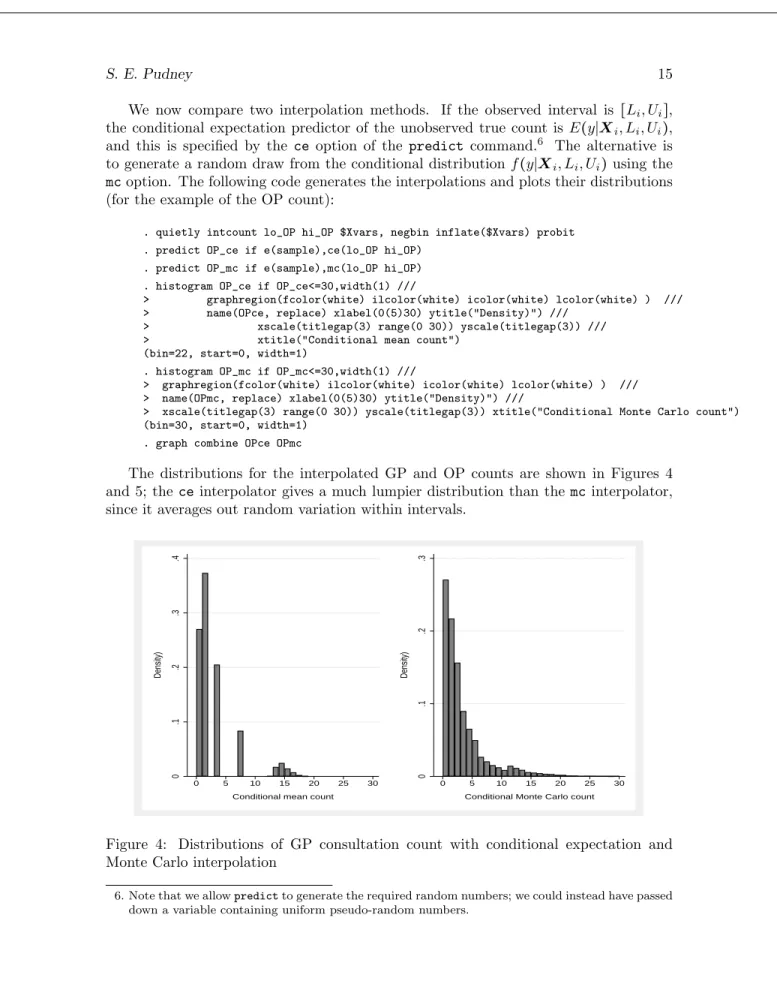
The distributions for the interpolated GP and OP counts are shown in Figures 4 and 5; theceinterpolator gives a much lumpier distribution than themcinterpolator, since it averages out random variation within intervals.
0 .1 .2 .3 .4 Density) 0 5 10 15 20 25 30 Conditional mean count
0 .1 .2 .3 Density) 0 5 10 15 20 25 30 Conditional Monte Carlo count
Figure 4: Distributions of GP consultation count with conditional expectation and Monte Carlo interpolation
6. Note that we allowpredictto generate the required random numbers; we could instead have passed down a variable containing uniform pseudo-random numbers.
0 .2 .4 .6 Density) 0 5 10 15 20 25 30 Conditional mean count
0 .2 .4 .6 Density) 0 5 10 15 20 25 30 Conditional Monte Carlo count
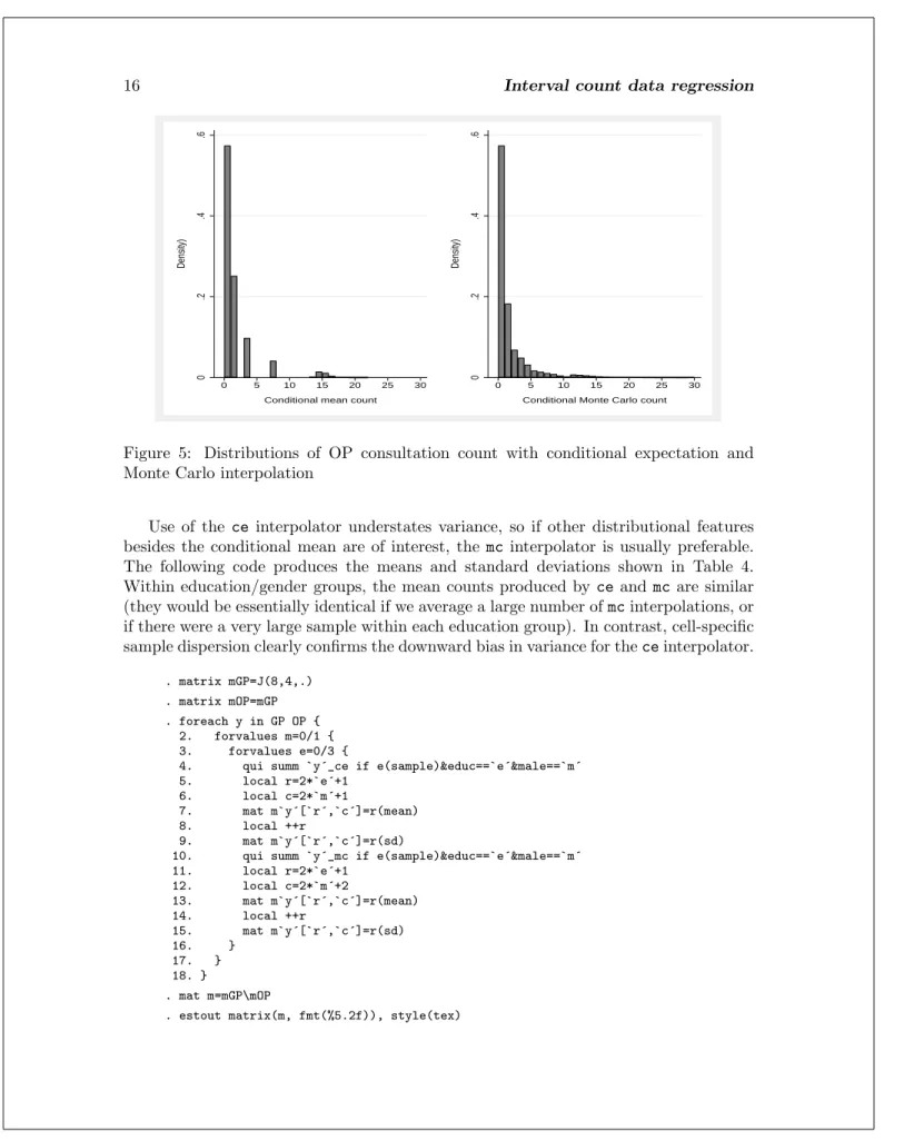
Figure 5: Distributions of OP consultation count with conditional expectation and Monte Carlo interpolation
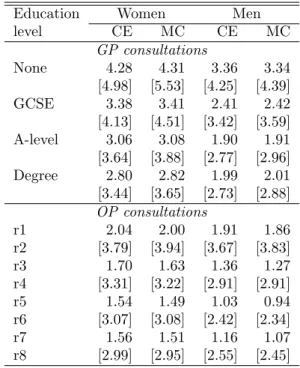
Use of the ceinterpolator understates variance, so if other distributional features besides the conditional mean are of interest, the mcinterpolator is usually preferable. The following code produces the means and standard deviations shown in Table 4. Within education/gender groups, the mean counts produced byceand mcare similar (they would be essentially identical if we average a large number ofmcinterpolations, or if there were a very large sample within each education group). In contrast, cell-specific sample dispersion clearly confirms the downward bias in variance for theceinterpolator.
. matrix mGP=J(8,4,.) . matrix mOP=mGP . foreach y in GP OP {
2. forvalues m=0/1 { 3. forvalues e=0/3 {
4. qui summ `y´_ce if e(sample)&educ==`e´&male==`m´ 5. local r=2*`e´+1
6. local c=2*`m´+1
7. mat m`y´[`r´,`c´]=r(mean) 8. local ++r
9. mat m`y´[`r´,`c´]=r(sd)
10. qui summ `y´_mc if e(sample)&educ==`e´&male==`m´ 11. local r=2*`e´+1 12. local c=2*`m´+2 13. mat m`y´[`r´,`c´]=r(mean) 14. local ++r 15. mat m`y´[`r´,`c´]=r(sd) 16. } 17. } 18. } . mat m=mGP\mOP
Table 4: Means and standard deviations of GP and hospital OP consultations interpo-lated by alternative methods.
Education Women Men
level CE MC CE MC GP consultations None 4.28 4.31 3.36 3.34 [4.98] [5.53] [4.25] [4.39] GCSE 3.38 3.41 2.41 2.42 [4.13] [4.51] [3.42] [3.59] A-level 3.06 3.08 1.90 1.91 [3.64] [3.88] [2.77] [2.96] Degree 2.80 2.82 1.99 2.01 [3.44] [3.65] [2.73] [2.88] OP consultations r1 2.04 2.00 1.91 1.86 r2 [3.79] [3.94] [3.67] [3.83] r3 1.70 1.63 1.36 1.27 r4 [3.31] [3.22] [2.91] [2.91] r5 1.54 1.49 1.03 0.94 r6 [3.07] [3.08] [2.42] [2.34] r7 1.56 1.51 1.16 1.07 r8 [2.99] [2.95] [2.55] [2.45]
Group-specific standard deviations in square brackets.
4.3
Determinants of future healthcare demand
The UKHLS is a perpetual panel and, in addition to healthcare use in wave 7, we can also observe a range of health measures and other characteristics at the wave 2 baseline. We use this rather than wave 1 as the baseline because a range of objective measurements was made by nurse interviewers at wave 2.
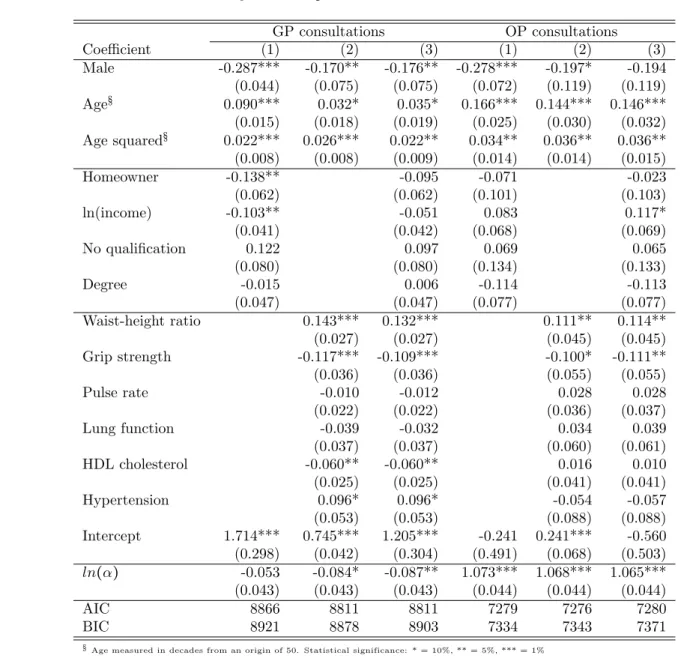
Our analysis dataset covers demographic covariates (age, gender); indicators of socio-economic status (SES) (homeownership, log equivalised household income, education); and biometrics (waist-height ratio, grip strength, resting heart rate, lung function, HDL “good” cholesterol, hypertension). We estimate standard negative binomial models from the interval data on GP and OP consultations. The following code produces three variants of the model for each dependent variable, and the parameter estimates are shown in Table 5:
. global Xdem "male a a2"
. global Xses "h_own ln_income noed degree" . global Xbio "whr grip pulse htfvc hdl hyper"
. qui reg lo_GP lo_OP $Xdem $Xses $Xbio . cap drop insamp
. gen byte insamp=e(sample)
. qui intcount lo_GP hi_GP $Xdem $Xses if insamp, negbin . estimates store GP1
. qui intcount lo_GP hi_GP $Xdem $Xbio if insamp, negbin . estimates store GP2
. qui intcount lo_GP hi_GP $Xdem $Xses $Xbio if insamp, negbin . estimates store GP3
. qui intcount lo_OP hi_OP $Xdem $Xses if insamp, negbin . estimates store OP1
. qui intcount lo_OP hi_OP $Xdem $Xbio if insamp, negbin . estimates store OP2
. qui intcount lo_OP hi_OP $Xdem $Xses $Xbio if insamp, negbin . estimates store OP3
. estout GP1 GP2 GP3 OP1 OP2 OP3, cells(b(star fmt(%7.3f)) /// > se(par)) starlevels(* .1 ** .05 *** .01) style(tex) /// > stats( aic bic, fmt(%7.0f) )
There is little evidence of a predictive role for SES variables when the biometrics are included in the model, so we adopt variant (2) which uses only demographic and biometric covariates. Among the biometrics, only waist-height ratio and grip strength have a consistently significant impact and the following code uses thenpredict option to quantify those impacts by computing the mean predicted effect of adding 1 standard deviation to each in turn. The effects are substantial in terms of the potential cost to the public health care system: a uniform 1 standard deviation increase in weight-height ratio increases the consultation workload by 15% for GPs and 12% for hospital out-patient clinics. A similar increase in the grip strength measure is predicted to produce an 11% reduction in GP workloads and a 10% reduction for out-patient clinics.
. foreach c in GP OP { 2. foreach x in whr grip { 3. cap drop pred*
4. estimates restore `c´2 5. cap drop tmp
6. qui gen double tmp=`x´ 7. qui predict pred0 if insamp,n 8. qui summ pred0,meanonly 9. scalar t0=r(mean) 10. qui replace `x´=`x´+1
11. qui predict pred1 if insamp,n 12. qui summ pred1,meanonly 13. scalar t1=r(mean) 14. di in gr "`c´: Impact of 1 sd increase in `x´: " %7.3f (t1-t0) 15. di in gr "Proportionate increase: " %5.1f 100*(t1-t0)/t0 "%" 15. qui replace `x´=tmp 16. } 17. }
(results GP2 are active now)
GP: Impact of 1 sd increase in whr: 0.344 ( 15.4%) (results GP2 are active now)
GP: Impact of 1 sd increase in grip: -0.246 (-11.0%) (results OP2 are active now)
(results OP2 are active now)
OP: Impact of 1 sd increase in grip: -0.126 ( -9.5%)
Table 5: 5-year ahead predictive models of healthcare use
GP consultations OP consultations Coefficient (1) (2) (3) (1) (2) (3) Male -0.287*** -0.170** -0.176** -0.278*** -0.197* -0.194 (0.044) (0.075) (0.075) (0.072) (0.119) (0.119) Age§ 0.090*** 0.032* 0.035* 0.166*** 0.144*** 0.146*** (0.015) (0.018) (0.019) (0.025) (0.030) (0.032) Age squared§ 0.022*** 0.026*** 0.022** 0.034** 0.036** 0.036** (0.008) (0.008) (0.009) (0.014) (0.014) (0.015) Homeowner -0.138** -0.095 -0.071 -0.023 (0.062) (0.062) (0.101) (0.103) ln(income) -0.103** -0.051 0.083 0.117* (0.041) (0.042) (0.068) (0.069) No qualification 0.122 0.097 0.069 0.065 (0.080) (0.080) (0.134) (0.133) Degree -0.015 0.006 -0.114 -0.113 (0.047) (0.047) (0.077) (0.077) Waist-height ratio 0.143*** 0.132*** 0.111** 0.114** (0.027) (0.027) (0.045) (0.045) Grip strength -0.117*** -0.109*** -0.100* -0.111** (0.036) (0.036) (0.055) (0.055) Pulse rate -0.010 -0.012 0.028 0.028 (0.022) (0.022) (0.036) (0.037) Lung function -0.039 -0.032 0.034 0.039 (0.037) (0.037) (0.060) (0.061) HDL cholesterol -0.060** -0.060** 0.016 0.010 (0.025) (0.025) (0.041) (0.041) Hypertension 0.096* 0.096* -0.054 -0.057 (0.053) (0.053) (0.088) (0.088) Intercept 1.714*** 0.745*** 1.205*** -0.241 0.241*** -0.560 (0.298) (0.042) (0.304) (0.491) (0.068) (0.503) ln(α) -0.053 -0.084* -0.087** 1.073*** 1.068*** 1.065*** (0.043) (0.043) (0.043) (0.044) (0.044) (0.044) AIC 8866 8811 8811 7279 7276 7280 BIC 8921 8878 8903 7334 7343 7371
5
Conclusions
Survey count data often come in interval form rather than exact counts. It is com-mon forad hoc methods to be used for modelling such data – for example, regression applied to mid-point interpolations, or ordered probit regression that does not exploit the known interval limits or the count nature of the data. This article documents a new Stata command,intcount, which allows the estimation of a range of count data regression models from interval data without making arbitrary approximations. The post-estimation predict command allows the use of the estimated model for a vari-ety of prediction purposes, including interpolation of the unobserved underlying exact count.
The use of the command is illustrated with applications to data from the UK Un-derstanding Society panel on the health service use. These applications demonstrate that interval observation need not be a barrier to econometric analysis.
6
Acknowledgements
I am grateful to Apostolos Davillas for help with preparing data from Understanding Society, which is an initiative funded by the Economic and Social Research Council and various Government Departments, with scientific leadership by the Institute for Social and Economic Research, University of Essex, and survey delivery by NatCen Social Research and Kantar Public. The research data are distributed by the UK Data Service. This work was supported by the Economic and Social Research Council through the project How can biomarkers and genetics improve our understanding of society and health? (grant ES/M008592/1), the Centre for Micro-Social Change (grant ES/L009153/1) and theUnderstanding Societystudy (grant ES/K005146/1). The views expressed in this article, and any errors or omissions, are mine alone.
7
References
Cameron, A. C., and P. K. Trivedi. 2013. Regression Analysis of Count Data (2nd ed.). Cambridge, UK: Cambridge University Press.
Davillas, A., and S. E. Pudney. 2019. Baseline health and public healthcare costs five years on: A predictive analysis using biomarker data in a prospective household panel. University of Essex,Understanding Society Working Paper no. 2019-01.
Manski, C. F., and E. Tamer. 2002. Inference on Regressions with Interval Data on a Regressor or Outcome. Econometrica70: 519–546.
StataCorp. 2017. Mata Reference Manual, Release 15. College Station, Texas. About the author
Steve Pudney is Professor of Health Econometrics in the Health Economics and Decision Science section in ScHARR, University of Sheffield, UK.