Parameter inference for multivariate stochastic processes with jumps

OpenBU http://open.bu.edu

Theses & Dissertations Boston University Theses & Dissertations

2016

Parameter inference for

multivariate stochastic processes

with jumps

https://hdl.handle.net/2144/17713 Boston University

GRADUATE SCHOOL OF ARTS AND SCIENCES

Dissertation

PARAMETER INFERENCE FOR MULTIVARIATE

STOCHASTIC PROCESSES WITH JUMPS

by

FRANC

¸ OIS GUAY

M.Sc.Eng., Ecole Nationale Sup´

erieure d’Arts et M´

etiers, 2010

M.Sc., Ecole Polytechnique de Montr´

eal, 2010

Submitted in partial fulfillment of the

requirements for the degree of

Doctor of Philosophy

2016

First Reader

Zhongjun Qu

Associate Professor of Economics

Second Reader

Gustavo Schwenkler

Assistant Professor of Finance

Third Reader

Pierre Perron

Many people have supported me throughout my doctoral studies, and I am extremely grateful to them.

First and foremost, I want to express my deepest gratitude to my advisers, Zhongjun Qu, Gustavo Schwenkler and Pierre Perron for their excellent mentor-ship. Zhongjun has been a very helpful and kind adviser. He taught me financial econometrics and encouraged me to pursue my research in that direction. His guid-ance has been invaluable. I would also like to thank Gustavo for his advice, patience and support. His passion for research has truly been inspiring. Moreover, his will-ingness and availability to spend time with me discussing our project has helped me grow and significantly improve my research skills. Finally, I am indebted to Pierre, who is one of the main reasons why I chose to come to BU in the first place. Pierre taught me most of what I know about econometrics, and he is a dedicated professor. I am truly honored to have him on my dissertation committee.

In addition to my advisers, I would like to thank Hiroaki Kaido and Iv´an Fern´ an-dez-Val for reading this thesis and for their feedback during the Econometrics semi-nar. A big thank you to Randy Ellis who was tremendously helpful as our placement coordinator. I would also like to thank Eric Jacquier for our discussions. He taught me MCMC methods and his research inspired me. Finally, I want to acknowledge the Hariri Institute for Computing and Computational Science & Engineering for their financial support.

Many other members of the Economics Department also contributed to this thesis. Thank you, Gloria, for all your help during the job application process. You made it much easier for me. Thank you, Andy, for being such a great coordinator for our program. Thank you, Deb, for these moments of chat and the candies. Finally, thank

This journey would have been different without my friends in the program. We started it together, and being surrounded by brilliant people helped me get through the good days and the hard days. Thank you Will, Svet, Calvin, Crystal, Matt, Jerry and the others for these relaxing lunches we had together. I am also grateful to the participants of the econometrics reading group. A special thanks to Julian, who has always been available to help me with the technical details of my thesis. Finally, thank you Fan, for our discussions and exchange of ideas on the third chapter of this thesis, and for making it through the job market with me!

Last but not least, I want to thank my family - my parents for having supported me since the beginning of my studies; Marianne, for being a great sister and always showing interest in my research; Mathilde, for being an awesome sister-in-law, always making me laugh whenever I needed to. Finally, I thank my wife, Anne-Sophie, for her unconditional support. I always admired your intellect, you have been a source of inspiration since I embarked on this journey. You always pushed me to reach for the stars, and I would have never done it without your support.

STOCHASTIC PROCESSES WITH JUMPS

FRANC

¸ OIS GUAY

Boston University, Graduate School of Arts and Sciences, 2016

Major Professors: Zhongjun Qu, Associate Professor of

Economics

Gustavo Schwenkler, Assistant Professor of

Finance

ABSTRACT

This dissertation addresses various aspects of estimation and inference for multi-variate stochastic processes with jumps.

The first chapter develops an unbiased Monte Carlo estimator of the transition density of a multivariate jump-diffusion process. The drift, volatility, jump inten-sity, and jump magnitude are allowed to be state-dependent and non-affine. The density estimator proposed enables efficient parametric estimation of multivariate jump-diffusion models based on discretely observed data. Under mild conditions, the resulting parameter estimates have the same asymptotic behavior as maximum likelihood estimators as the number of data points grows, even when the sampling frequency of the data is fixed. In a numerical case study of practical relevance, the density and parameter estimators are shown to be highly accurate and computation-ally efficient.

In the second chapter, I examine continuous-time stochastic volatility models with jumps in returns and volatility in which the parameters governing the jumps are allowed to switch according to a Markov chain. I estimate the parameters and

Markov-switching parameters characterize well the periods of market stress, such as those in 1997-1998, 2001 and 2007-2010. Several statistical tests favor the model with Markov-switching jump parameters. These results provide empirical evidence about the state-dependent and time-varying nature of asset price jumps, a feature of asset prices that has recently been documented using high-frequency data.

The third chapter considers applying Markov-switching affine stochastic volatil-ity models with jumps in returns and volatilvolatil-ity, where the jump parameters are not regime-switching. The estimation is performed via Markov Chain Monte Carlo meth-ods, allowing to obtain the latent processes induced by the structure of the models. Furthermore, I propose some misspecification tests and develop a Markov-switching test based on the odds ratios. The parameters and the latent processes are estimated using the S&P 500 index from 1970 to 2014. I show that the S&P 500 stochastic volatility exhibits a Markov-switching behavior, and that most of the high volatility regimes coincide with the recessions identified ex-post by the National Bureau of Economic Research.

1 Efficient Parameter Estimation for Multivariate Jump-Diffusions 1 1.1 Introduction . . . 1 1.1.1 Related methods . . . 5 1.2 Problem formulation . . . 9 1.2.1 Inference problem . . . 10 1.3 Density representation . . . 12 1.4 Density estimator . . . 15

1.4.1 Towards an unbiased estimator . . . 16

1.4.2 Estimator . . . 20

1.5 Computation of the density estimator . . . 22

1.5.1 Ensuring a finite variance . . . 22

1.5.2 Computational properties . . . 25 1.5.3 Implementation . . . 29 1.6 Parameter inference . . . 31 1.7 Numerical results . . . 33 1.7.1 Density estimator . . . 35 1.7.2 Computational complexity . . . 36

1.7.3 Simulated likelihood estimators . . . 37

2 Stochastic Volatility Models with Markov-Switching Jump Param-eters 47 2.1 Introduction . . . 47

2.2 Markov-switching jump-diffusion models . . . 50

2.3.1 The MCMC algorithm . . . 55 2.3.2 Model diagnoses . . . 56 2.3.3 Simulation results . . . 57 2.4 Empirical results . . . 60 2.4.1 SVMSJ model . . . 61 2.4.2 SVMSCJ model . . . 64 2.4.3 SVMSIJ model . . . 67 2.4.4 Markov-switching diagnoses . . . 70

2.4.5 Markov-switching jump parameters . . . 70

2.5 Conclusion . . . 71

3 Affine Stochastic Volatility Models with Regime-Switching 85 3.1 Introduction . . . 85

3.2 Models . . . 88

3.3 Estimation method . . . 90

3.3.1 Introduction to MCMC . . . 90

3.3.2 Posterior and prior distributions . . . 91

3.3.3 Gibbs algorithm . . . 92

3.4 Model diagnoses and specification tests . . . 93

3.5 Numerical results . . . 97

3.5.1 Simulated data . . . 97

3.5.2 Empirical results . . . 102

3.6 Conclusion . . . 108

A.1 Algorithms . . . 116

A.2 Proofs . . . 117

B Proofs for Chapter 2 128 B.1 Posterior distribution computations . . . 128

B.1.1 The model . . . 128 B.1.2 Posterior distribution of ξv . . . 129 B.1.3 Posterior distribution of ξy . . . 134 B.1.4 Posterior distribution of N . . . 136 B.1.5 Posterior distribution of S . . . 138 B.1.6 Posterior distribution of Θ . . . 138

B.1.7 Posterior distribution of the volatility . . . 151

C Proofs for Chapter 3 152 C.1 Posterior distribution computations . . . 152

C.1.1 The model . . . 152 C.1.2 Posterior distribution of ξv _{. . . 153} C.1.3 Posterior distribution of ξy . . . 158 C.1.4 Posterior distribution of N . . . 160 C.1.5 Posterior distribution of S . . . 161 C.1.6 Posterior distribution of Θ . . . 162

C.1.7 Posterior distribution of the volatility . . . 174

Bibliography 175

Curriculum Vitae 181

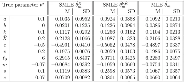
1.1 Simulated likelihood, biased simulated likelihood and true likelihood

estimators . . . 38

1.2 Asymptotic distribution of the SMLE θ_mK . . . 39

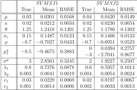
2.1 Simulation study for the models with jumps in returns . . . 58

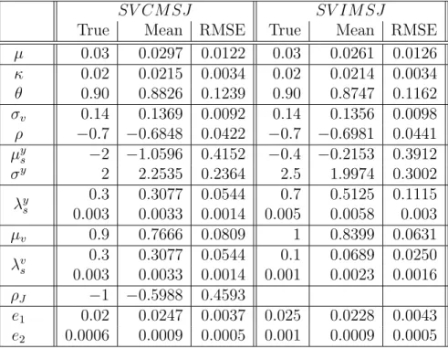
2.2 Simulation study for the models with jumps in returns and volatility 59 2.3 Summary statistics for S&P 500 and Nasdaq returns, 1990-2014 . . . 61

2.4 Parameter comparison for theSV J and SV M SJ models . . . 62

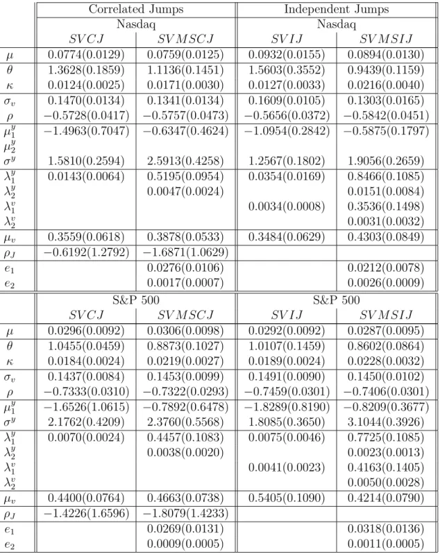
2.5 Parameter comparison for theSV CJ and SV M SCJ models . . . 66

2.6 Parameter comparison for theSV IJ and SV M SIJ models . . . 69

2.7 Odds ratios . . . 70

2.8 Variance decomposition for the three classes of models . . . 71

3.1 Simulation study for the models with jumps in returns . . . 99

3.2 Simulation study for the models with correlated jumps in returns and volatility . . . 100

3.3 Simulation study for the models with independent jumps in returns and volatility . . . 101

3.4 Simulated study of the odds ratios . . . 102

3.5 Summary statistics for the S&P 500 index, 1970-2014 . . . 102

3.6 Parameter estimation for the models with jumps in returns, S&P 500 103 3.7 Parameter estimation for the models with correlated jumps in returns and volatility, S&P 500 . . . 104

turns and volatility, S&P 500 . . . 105 3.9 Odds ratios . . . 108

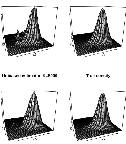
1.1 Surface plots . . . 40

1.2 Contour plots . . . 41

1.3 Marginal density of returns . . . 42

1.4 Marginal density of volatility . . . 43

1.5 Conditional density of returns . . . 44

1.6 Conditional density of volatility . . . 45

1.7 Computational efficiency . . . 46

2.1 Prices and returns for the S&P500 and Nasdaq indices . . . 73

2.2 Nasdaq latent variables for the models with jumps in returns . . . 74

2.3 Nasdaq stochastic volatility for the models with jumps in returns . . 75

2.4 S&P 500 latent variables for the models with jumps in returns . . . . 76

2.5 Residuals of the models with jumps in returns . . . 77

2.6 QQplots of the Nasdaq residuals for the models with jumps in returns 78 2.7 QQplots of the S&P 500 residuals for the models with jumps in returns 79 2.8 Nasdaq latent quantities for the models with correlated jumps in re-turns and volatility . . . 80

2.9 S&P 500 latent variables for the models with correlated jumps in re-turns and volatility . . . 81

2.10 Residuals of the models with correlated jumps in returns and volatility 82 2.11 Nasdaq latent quantities for the models with independent jumps in returns and volatility . . . 83

2.12 S&P 500 latent variables for the models with independent jumps in returns and volatility . . . 84

3.2 Latent variables . . . 111 3.3 S&P 500 returns and latent variables . . . 112 3.4 Stochastic volatility and Markov-switching parameterθ . . . 113 3.5 Comparison of latent variables, S&P 500 returns and the VIX . . . . 114 3.6 Bear indicator and NBER recessions . . . 115

DGP . . . Data Generating Process

GMM . . . Generalized Method of Moments MCMC . . . Markov Chain Monte Carlo MLE . . . Maximum Likelihood Estimator

N0 . . . the set of natural numbers, including 0

NBER . . . National Bureau of Economic Research QMLE . . . Quasi Maximum Likelihood Estimation

R+ . . . the set of positive real numbers

Rd . . . Euclidean space of dimension d

SMLE . . . Simulated Maximum Likelihood Estimator

Chapter 1

Efficient Parameter Estimation for Multivariate

Jump-Diffusions

1.1

Introduction

Multivariate jump-diffusions are popular stochastic processes often used in economic and financial applications. They describe the time series behavior of asset prices, volatilities, and interest rates, as well as the correlation structure of the cross section of assets. They also allow for potential discontinuities in the time series of financial and economic data. Despite their popularity, parameter inference for multivariate jump-diffusions is challenging because the underlying probability distribution is of-tentimes intractable.

In this chapter, we derive an unbiased Monte Carlo estimator of the transition density of a general class of multivariate jump-diffusion processes over arbitrary sam-ple frequencies. The resulting density estimator can be used to perform maximum likelihood inference based on discretely observed data. Under conditions that can be verified using this density estimator, the parameter estimators inherit the con-sistency and asymptotic normality properties of maximum likelihood estimators as the number of data points grows large.2 _{Thus, the results of this chapter provide a}

methodology to carry out statistically efficient estimation of the parameters driving the dynamics of a multivariate jump-diffusion process based on discretely observed data.

1_{This chapter is based on a joint work with Gustavo Schwenkler.}

We consider a general class of Markovian multivariate jump-diffusions. The drift, volatility, jump intensity, and jump magnitude are allowed to be arbitrary paramet-ric functions of the state. The only binding assumption is that the jump-diffusion process is well-defined in the sense that it admits a strong solution as well as a transition density. By taking advantage of Bayes’ rule and a well-chosen change of measure, we rewrite the transition density of a multivariate jump-diffusion in terms of a mixture of transition densities of purely diffusive processes without jumps. Our methodology is similar to the one of Giesecke and Schwenkler (2014), who charac-terize the transition density of a jump-diffusion as a mixture of Gaussian densities. In contrast to Giesecke and Schwenkler (2014), our density representation also ap-plies to multivariate jump-diffusion processes which are not reducible in the sense of A¨ıt-Sahalia (2008). A process is reducible if it can be transformed to a unit volatil-ity process, and this restrictive assumption is often violated by popular multivariate jump-diffusion models.3 _{Our density representation also provides a significant}

gener-alization of the well-known representations of Dacunha-Castelle and Florens-Zmirou (1986) and Rogers (1985), which apply only to univariate diffusive processes without jumps.

A key benefit of our density representation is that it can be easily estimated via Monte Carlo simulation, because it is given by an unconditional expectation of a path functional of the jump-diffusion process. We exploit a novel randomization technique introduced by Glynn and Rhee (2015) to construct an unbiased estimator of the transition density. This density estimator can be understood as a randomized multilevel Monte Carlo estimator.4 _{It is constructed from samples derived from}

Euler’s discretization method with different time steps, which are mixed and weighted

3_{e.g., affine stochastic volatility models.}

adequately to ensure unbiasedness of the density estimator.5 _{The accuracy of the}

resulting estimator depends only on the number of Monte Carlo replications used. We use the density estimator to carry out parameter inference based on discretely observed data. We construct a simulated likelihood function by replacing the un-computable true density with our density estimator. Because the latter is unbiased, standard results ensure that the estimators that maximize the simulated likelihood inherit the asymptotic properties of true maximum likelihood estimators as the num-ber of data points grows large while keeping the observation frequency of the data fixed.6 _{Under conditions that can be verified using our density formulation, the}

simulated maximum likelihood estimator converges to a true maximum likelihood estimator as the number of Monte Carlo replications grows large while keeping the data sample fixed. When the number of Monte Carlo replications grows and the number of data points grows, standard conditions ensure that the simulated likeli-hood estimator is consistent. Furthermore, if the number of Monte Carlo replications grows at the same rate as the data grows, then a simulated maximum likelihood esti-mator is asymptotically normal with the same asymptotic variance-covariance matrix as a true maximum likelihood estimator. As a result, our simulated likelihood esti-mators are asymptotically efficient in the sense that they have the same asymptotic standard errors as true maximum likelihood estimators.

An important property of the simulated likelihood estimators we propose is that, even though they are derived from Monte Carlo simulation, their asymptotic variance-covariance matrix is the same as that of true maximum likelihood estima-tors. This means that the Monte Carlo methodology we use to estimate the transition

5_{See Kloeden and Platten (1999) for an overview of Euler’s method.}

6_{We do not consider infill asymptotic regimes, in which the time between consecutive}

density does not affect the asymptotic distribution of the resulting parameter esti-mators. The reason why this key property holds is that our density estimator is unbiased. Were it not unbiased, then its bias would be transferred to the parameter estimators either by making them inconsistent or asymptotically inefficient. Detem-ple et al. (2006) establish this result in the diffusion case, and we conjecture that the same holds in the jump-diffusion case. Overall, the fact that our density estimator is unbiased is the main property that enables efficient parameter estimation in this chapter.

Our framework has important computational features. The transition density can be evaluated at any value of the parameter and arguments of the density function without re-simulation. A single set of Monte Carlo replications suffices to evaluate it at different arguments. This property entails significant computational benefits when carrying out parameter inference, especially for large data sets. It reduces the simulated likelihood maximization problem to a deterministic problem that can be solved using standard methods. Furthermore, our density estimator can be fine-tuned to minimize its variance for a given number of Monte Carlo replications. This feature makes it highly accurate in practical applications. Moreover, our methodology is based on Euler’s discretization method with different time steps, therefore several Brownian increments can be re-used when carrying out Euler discretization. This property simplifies the computational work. Finally, given that our framework hinges on independent Monte Carlo replications, computations can be easily parallelized, yielding further computation benefits.

A numerical case study showcases the benefits of our density estimator and sim-ulated likelihood estimators. We consider a stochastic volatility model with jumps in returns and volatility. The distribution of returns is non-Gaussian, and the

dis-tribution of volatility is asymmetric and skewed. This bivariate affine model has the advantage that its transition density is known in closed-form. It can be recovered by Fourier inversion of the characteristic function as in Duffie et al. (2000). Because of these properties, the stochastic volatility model provides an appropriate case study to assess the performance of our estimation methodology. The numerical results show that our density estimator is highly accurate. It is able to capture the non-Gaussian distribution of returns, as well as the asymmetric distribution of volatility, both in the centers and the tails of the distributions. The density estimator becomes more accurate as the number of Monte Carlo replications grows large. It beats a naive biased density estimator derived from Euler’s method in terms of accuracy achieved using medium to high computational budgets. The resulting simulated likelihood estimators are also found to be highly accurate. They are able to closely recover the data-generating parameters, on the contrary to likelihood estimators obtained via a biased density estimator.

1.1.1 Related methods

The methodology of this chapter offers several advantages for parameter inference, that alternative approaches generally do not satisfy.

The method closest to ours is the one of Giesecke and Schwenkler (2014), who estimate the transition density of reducible jump-diffusions using exact simulation techniques. The density estimator of Giesecke and Schwenkler (2014) is compu-tationally efficient for large computational budgets, and unbiased. Therefore, the parameter estimators of Giesecke and Schwenkler (2014) also inherit the asymptotic properties of maximum likelihood estimators. Their method is targeted primarily towards univariate jump-diffusions, which are reducible under mild conditions.

How-ever, even some of the most basic multivariate jump-diffusions are irreducible. For example, the standard stochastic volatility model of Heston (1993) is not reducible. Unlike the estimators of Giesecke and Schwenkler (2014), ours are applicable to the class of irreducible multivariate jump-diffusions.

If the model is affine as in Duffie et al. (2000), the transition density can be recov-ered via Fourier inversion of the characteristic function, which satisfies a system of ordinary differential equations. However, solving these ordinary differential equations and carrying out Fourier inversion numerically is computationally challenging in the multivariate case. Lo (1988) recovers the transition density of a jump-diffusion pro-cess with constant jump intensity and state-independent jump magnitudes by solving the Fokker-Planck equations governing it. This method is computationally burden-some for large data sets because the corresponding partial differential equations need to be solved recursively across data points. In addition, the numerical solution of the Fokker-Planck equations suffers from the curse of dimensionality, making it un-suitable for multivariate applications. In contrast to the methods of Duffie et al. (2000) and Lo (1988), our density estimator also applies for non-affine models with state-dependent jumps.

Inspired by the work of A¨ıt-Sahalia (2002), Yu (2007) derives a small-time expan-sion approximation of the transition density of a multivariate jump-diffuexpan-sion process with state-independent jump sizes. The coefficients of his expansion satisfy a set of interdependent partial differential equations. Solving these partial differential equa-tions is computationally burdensome when the number of expansion terms is large, and when the jump-diffusion process is not reducible. The parameter estimators derived from the density estimator of Yu (2007) inherit the asymptotic properties of maximum likelihood estimator when the time between consecutive observations

shrinks to zero as more data points become available. In contrast, our simulated like-lihood estimators inherit the asymptotic properties of maximum likelike-lihood estimators under standard conditions as the number of data points grows while keeping the ob-servation frequency of the data fixed. This type of asymptotic regime is common in many econometric applications.7 Furthermore, the computational effort necessary to evaluate our density estimator does not depend on the reducibility of the process.

Kristensen and Shin (2012) derive nonparametric estimators of the transition den-sity of a jump-diffusion process with state-independent coefficient functions.8 _These

authors apply a kernel estimator to samples of the jump-diffusion process derived from Euler discretization. If the bandwidth of the kernel estimator shrinks to zero as the number of data points grows large, then the parameter estimators derived from their density estimator inherit the asymptotic properties of maximum likeli-hood estimators. Their density estimator and ours are similarly inexpensive from a computational point of view. However, in contrast to Kristensen and Shin (2012), our density estimator also applies to jump-diffusions with state-dependent coefficient functions.

Moment-based methods can also be used for parameter inference. Jiang and Knight (2002), Chacko and Viceira (2003), Duffie and Glynn (2004), and Duffie and Singleton (1993) propose generalized method of moments estimators for continuous-time Markov processes. Should an infinite number of moments be used to perform estimation, then the moment-based parameter estimators inherit the asymptotic properties of maximum likelihood estimators as the number of data points grows large. However, the use of an infinite number of moments is infeasible in practical

7_{Bibby and Sørensen (1995), Florens-Zmirou (1989), Giesecke and Schwenkler (2014), and Gobet}

et al. (2004) consider similar asymptotic regimes.

8_{The assumption that the distribution of}

tis independent oftandθin equation (1) of Kristensen

applications.9

Gourieroux et al. (1993) and Smith (1993) propose methods of indirect inference that are also applicable for multivariate jump-diffusions. Indirect inference requires that one is able to simulate from the jump-diffusion model. In addition, it requires that one specifies an auxiliary model. If the latter is correctly specified, then the pa-rameter estimators derived from indirect inference inherit the asymptotic properties of maximum likelihood estimators. Unlike indirect inference, our estimation method-ology does not require the specification of auxiliary models, and our simulated likeli-hood estimators inherit the asymptotic properties of maximum likelilikeli-hood estimators under conditions that can be verified using our density estimator. Furthermore, our methodology is applicable for a general class of multivariate jump-diffusions. This is not the case for indirect inference because the exact simulation of multivariate jump-diffusions is infeasible unless the process is reducible.10

The rest of this chapter is organized as follows. Section 1.2 formulates the model and the estimation problem. In Section 1.3, we derive our density representation. We introduce the density estimator in Section 1.4, and discuss its computational properties in Section 1.5. Section 1.6 proposes simulated likelihood estimators and summarizes their asymptotic properties. A numerical case study is carried out in Section 1.7.

9_{There are few cases in which maximum likelihood efficiency can be achieved with a finite number}

of moments. See, e.g., Carrasco et al. (2007) and Jiang and Knight (2010).

10_{We refer to Giesecke and Smelov (2013) for the exact simulation of reducible jump-diffusions.}

1.2

Problem formulation

Fix a complete probability space (Ω,F,_P) and a right-continuous, complete infor-mation filtration (Ft)t≥0. Let X be a jump-diffusion process valued in S ⊂Rd that

is governed by the stochastic differential equation

dXt =µ(Xt;θ)dt+ Σ(Xt;θ)dBt+ dLt, (1.1)

whereX0 ∈ S is fixed and known, µ:S ×Θ→Rd is the drift function, Σ :S ×Θ→

Rd×d is the positive definite volatility matrix function,B is a standardd-dimensional

Brownian motion, and L is a jump process of the type

Lt = Nt

X

n=1

Γ(XTn−, Dn;θ) (1.2)

whereNtis a non-explosive counting process with event stopping times (Tn)n≥1 and

jump intensityλt= Λ(Xt;θ) for a function Λ :S ×Θ→R+. Here,Xt− = lims%tXs.

The jump magnitudes of the process X are determined by the function Γ : S × D ×Θ→_Rd_{. The mark variables (D}

n)n≥1, which characterize the jumps of X, are

independent and identically distributed in D ⊂ _R with probability density π. The drift, volatility, jump intensity, and jump size functions are specified by a parameter θ ∈Θ to be estimated, where the parameter space Θ is a subset of Euclidean space. Overall, X is a Markov process with infinitesimal generator for functionsf :_Rd →_R

with bounded and continuous first and second order derivatives given by: Aθf(x) = d X i=1 µi(x;θ) ∂f(x) ∂xi +1 2 X 1≤i,j≤d Σ(x;θ)Σ(x;θ)T i,j ∂2_f(x) ∂xixj + Λ(x;θ) Z D (f(x+ Γ(x, u;θ))−f(x))π(u)du.

We impose the following assumptions. First, the boundary ofSis either unattain-able or absorbing if attainunattain-able. Second, the parameter space Θ is a compact subset of_Rr with non-empty interior. Third, there exists a unique strong solution (X, J) of the above system; sufficient conditions are given in Protter (2004). We focus on the case of constant observation frequencies, i.e., ti −ti−1 = ∆ for all i, although all

re-sults hold for mixed observation frequencies as long as sup_i≥1|ti−ti−1|<∞. We also

assume for simplicity that the process N and the mark variables (Dn)n≥1 are

one-dimensional, and that the jump mark density π is parameter independent. Finally, we assume that X admits a transition density. Cass (2009), Filipovi´c et al. (2013), Komatsu and Takeuchi (2001), and Takeuchi (2002) provide sufficient conditions.

We use the following notation throughout the chapter. A subscript in _Pθ or Eθ

indicates that the parameter determining the law of the stochastic process X in (2.1) isθ. The gradient and the Hessian matrix operators are denoted by ∇and ∇2_,

respectively. For any 1 ≤ ν, ι, κ ≤ r, write ∂ν, ∂ν,ι2 , and ∂ν,ι,κ3 for the first, second,

and third partial derivatives with respect to θν, θι, and θκ.

1.2.1 Inference problem

Suppose that there exists a parameterθ∗ ∈int Θ such that the paths of Xsatisfy the SDE (2.1) for θ=θ∗. We say that θ∗ is the true parameter. Our goal is to estimate θ∗given a sequence of observations ofX sampled at the fixed and deterministic times

0 =t0 < . . . < tm <∞. We will use the method of maximum likelihood.

The dataXm ={Xt0, . . . , Xtm}is a random variable valued inS

m_{and measurable}

with respect toBm_{, whereBis the Borelσ-algebra onS. The likelihood of the data is}

the Radon-Nikodym density of the law of Xm with respect to the Lebesgue measure

on (Sm_,Bm_{). Lettingp}

t(x, .;θ) be the Radon-Nikodym density of the law ofXt given

X0 = x with respect to the Lebesgue measure on (S,B) (the transition density of

X), the likelihood of θ at the data Xm takes the form

Lm(θ) = m Y

i=1

p∆(Xti−1, Xti;θ) (1.3)

due to the Markovian structure of (2.1). The maximum likelihood estimator (MLE) satisfies

ˆ

θm ∈arg max

θ∈Θ Lm(θ) (1.4)

almost surely. We only consider interior MLEs that satisfy the first order condition

∇Lm(ˆθm) = 0. (1.5)

Maximum likelihood inference requires that one is able to evaluate the density p∆. This is generally not possible for the broad class of jump-diffusion models we

consider. We will therefore proceed to construct an unbiased estimator of the density p∆, and use this density estimator to compute maximum likelihood estimators based

1.3

Density representation

Consider the random variable

Z∆(θ) = exp   ∆ Z 0 (Λ(Xs;θ)−`) ds   N∆ Y n=1 ` Λ(XTn−;θ) (1.6)

for θ ∈Θ and ` >0. If _Eθ[Z∆(θ)] = 1, thenZ∆(θ) defines an equivalent probability

measure_Qθon (Ω,F∆) given byQθ[A] =Eθ[Z∆(θ)1A] for anyA ∈ F∆. The theorems

of L´evy and Watanabe imply that, under _Qθ and on [0,∆], N is a Poisson process

with rate `; see Br´emaud (1980). Consequently, jumps of the process X arrive at a constant rate under _Qθ. Between jump times, X follows a diffusive process without

jumps. These insights yield a novel representation of the density p∆, summarized in

the following theorem.

Theorem 1.3.1. Fix ` >0. Suppose the following assumptions hold.

(A1) For any θ ∈Θ, the variable Z∆(θ) has unit expectation, Eθ[Z∆(θ)] = 1.

(A2) For any θ ∈ Θ, the process (Xt :t ∈ [0,∆]) is a strong Markov process under

Qθ.

Let X˜ be the solution to the SDE

d ˜Xt=µ( ˜Xt;θ)dt+ Σ( ˜Xt;θ)d ˜Bt, X˜0 ∈ S, (1.7)

for a standard Brownian motion B˜ independent of B. Let p˜t(v,·;θ) denote the Pθ -transition density of X˜t given X˜0 =v.

Then, p∆(v, w;θ) =EQθ _p˜ ∆−TN_∆(XTN_∆, w;θ) Z∆(θ) X0 =v (1.8)

for any 0≤t ≤∆, v, w∈ S, and θ∈Θ.

The density representation of Theorem 1.3.1 consists of a mixture of transition densities of diffusion processes of the type (1.7). It is an implication of Bayes’ for-mula. Under Assumption (A2) and conditional on (N∆,(Tn)n≤N∆,(XTn)n≤N∆), that is, conditional on the number of jumps of X before time ∆, the realizations of all jump times before ∆, and the values of X at all jump times before ∆, the transition ofX from time 0 to time ∆ is governed only by the law ofX from the last jump time TN∆ until time ∆. Given that no jump occurs in the time interval (TN∆,∆], the law of X during this time interval is the same as the law of the diffusive process (1.7). As a result, under Assumption (A2) and conditional on (N∆,(Tn)n≤N∆,(XTn)n≤N∆), the density of X for a transition from v at time 0 to w at time ∆ is equal to the density ˜p∆−TN_∆(XTN_∆, w;θ) with X0 = v. Bayes’ formula tells us that we can

recover the unconditional density p∆ by integrating out according to the law of

(N∆,(Tn)n≤N∆,(XTn)n≤N∆). This is done by taking the expectation in (1.8). The term 1/Z∆(θ) in expression (1.8) accounts for the change of measure, which

sig-nificantly simplifies the estimation of the density in Section 1.4. Assumption (A1) guarantees that the change of measure is well-defined. It is a standard regularity assumption; Blanchet and Ruf (2013) give sufficient conditions. Assumption (A2) is also standard; see (Protter, 2004, Theorem 32). Finally, the diffusion density ˜pt

exists if the jump-diffusion density pt exists.

rep-resentation of Giesecke and Schwenkler (2014), who characterize the transition den-sity of the process as a mixture of Gaussian densities. This is possible because Giesecke and Schwenkler (2014) consider a transformation of the jump-diffusion pro-cess known as the Lamperti transform, which has unit volatility. When the under-lying process is univariate, the Lamperti transform exists under mild conditions. In the multivariate case, on the other hand, the Lamperti transform exists only when the process is reducible in the sense of A¨ıt-Sahalia (2008). As a result, the den-sity representation of Giesecke and Schwenkler (2014) is restricted to the class of reducible multivariate jump-diffusions.11 _{In contrast, we are not restricted to the}

class of models for which the Lamperti transform exists. Consequently, the density representation (1.8) also applies to irreducible processes. Many models of practical relevance are not reducible. For example, the stochastic volatility model of Heston (1993) is not reducible, but it is extensively used in the options pricing literature.12 Theorem 1.3.1 significantly extends the well-known density representations of Dacunha-Castelle and Florens-Zmirou (1986) and Rogers (1985). These representa-tions apply only in the univariate diffusion case; i.e., when Γ ≡ 0 and d = 1. In contrast, our density representation also applies in the multivariate jump-diffusion case.

The representation (1.8) also facilitates the derivation of conditions under which the transition density is smooth with respect to the parameterθ. Smoothness is nec-essary for consistency and asymptotic normality of maximum likelihood estimators. For smoothness of the density, we only require smoothness of the coefficient functions and an integrability condition, which can be verified using the density estimator we

11_{In the multivariate case, their density representation is further restricted to a smaller class}

of processes, because coarser conditions are needed to satisfy the change of variable operated in Section 3.1 of Giesecke and Schwenkler (2014).

introduce in Section 1.4. Our conditions for smoothness are easier to verify in practi-cal settings and less restrictive than alternative conditions, which oftentimes require that the coefficient functions have bounded derivatives of all orders (see, e.g., Cass (2009), Komatsu and Takeuchi (2001), and Takeuchi (2002)).

Proposition 1.3.2. Suppose that the conditions of Theorem 1.3.1 hold. Suppose also that the following conditions hold:

(A3) The partial derivatives up to n-th order of Φ∆(x, y;θ) = ˜p∆−TN_∆(x, y;θ)

1

Z∆(θ)

are uniformly bounded in expectation in the following sense: For all 1≤k ≤n

and q1, . . . , qk ∈ {θ1, . . . , θr, v, w}, EQθ sup θ∈Θ sup v,w∈S ∂k ∂q1. . . ∂qk ˜ p∆−TN_∆(v, w;θ) 1 Z∆(θ) <∞.

(A4) The drift function µ, volatility matrix function Σ, jump intensity function Λ,

jump magnitude function Γ, and diffusive density p˜ are n-times continuously

differentiable with respect to all of their arguments.

Then θ7→p∆(v, w;θ) is n-times continuously differentiable for any v, w∈ S.

1.4

Density estimator

Evaluating the transition density of the jump-diffusion X is challenging given that the law of X is intractable in many applications. A key advantage of the density representation (1.8) is that it can be efficiently approximated by exploiting a random-ization technique introduced by Glynn and Rhee (2015), which yields an unbiased density estimator. In this section, we introduce our density estimator, and analyze its convergence properties.

1.4.1 Towards an unbiased estimator

Under _Qθ, jumps of X arrive with constant intensity`. As a result, samples of N∆

can be simulated without bias using a standard inverse method. Conditional on N∆, the distribution of the jump times (Tn)n≤N∆ is the same as that of the order statistics of N∆ uniform random variables on [0,∆]. Samples of the jump times

(Tn)n≤N∆ conditional on N∆ can therefore also be simulated without bias. If the diffusive density ˜p is known in closed form, and samples of (XTN_∆,1/Z∆(θ)) can be

simulated without bias. Then,

˜

p∆−TN_∆(XTN_∆, w;θ)

Z∆(θ)

given X0 = v is an unbiased estimator of (1.8) that can be sampled exactly via

Monte Carlo simulation. In most applications, however, the diffusive density ˜p is not known in closed form, and one cannot sample exactly from the distribution of (XTN_∆,1/Z∆(θ)). We circumvent these issues by taking several steps, which we

summarize below.

1.4.1.1 Euler discretization

Note thatZ_∆−1(θ) is an exponential martingale that satisfies the following SDE under

Qθ: dZ_t−1(θ) =−Z_t−₋1(θ) Λ(Xt−;θ) ` −1 (`dt−dNt), Z0−1(θ) = 1. (1.9)

We can generate an approximation of (XTN_∆, Z

−1

∆ (θ)) using Euler discretization.

To do this, we first generate exact samples of N∆ and also samples of (Tn)n≤N∆ conditional on N∆. Between sampled jump times, we approximate the dynamics of

X andZ−1_{via Euler discretization withJ steps. Letting (X}J_{, Z}−J_{) denote the Euler}

discretization of (X, Z−1_{), we initialize X}J

0,0 =X0 and Z0−,0J = 1, and set

X_n,jJ =      XJ n,j−1+µ Xn,jJ −1;θ hn+ Σ Xn,jJ −1;θ Bjhn−B(j−1)hn , 1≤j ≤J, X_nJ_−1,J + Γ X_nJ_−1,J, Dn;θ , n >0, j = 0, Z_n,j−J =      Z_n,j−J₋₁−Z_n,j−J₋₁ Λ XJ n,j−1;θ −`hn, 1≤j ≤J, Λ(XJ n−1,J;θ) ` Z −J n−1,J, n >0, j = 0,

for 0 ≤ n ≤ N∆ and hn = Tn−_JTn−1, where we have used the notation T0 = 0 and

TN∆+1 = ∆ for simplicity. This construction ensures that the two Euler discretiza-tions between consecutive jump times are correctly pasted together by accounting for the jumps of X and Z−1_{. The nature of the Euler discretization implies that}

(XJ_,ZJ_{) = (X}J N∆,0, Z −J N∆,J) is a biased estimator of (XTN_∆, Z −1 ∆ (θ)). Consequently, ˜ p∆−TN_∆ X J , w;θZJ

is a biased estimator of the density p∆(v, w;θ) in (1.8).

1.4.1.2 Diffusion density

Next, we approximate the diffusion density ˜p. This can also be done via Euler discretization. For a given sample of (N∆, TN∆), we discretize the diffusive process

˜

X between time 0 and time ∆−TN∆ in an analogous way as for X

J_{, but using I}

Euler steps instead of J. Let ( ˜XI

i)0≤i≤I denote the Euler discretization of ˜X with

Euler step size ˜h = ∆−TN∆

I obtained this way. Conditional onTN∆ and ˜X

I

0, the law of

˜

distributed. More precisely, the conditional density of ˜XI I given TN∆ and ˜X I 0 =v is ˜ PI(v, w;θ) = Z I Y i=1 φ xi;xi−1,˜h dx1. . .dxI−1 (1.10)

where x0 = v, xI = w, and φ(·;x, h) is the density of the d-dimensional normal

distribution with meanx+µ(x;θ)hand variance-covariance matrixhΣ(x;θ)Σ>(x;θ). The mixed normal density (1.10) can be computed using standard numerical routines; see Section 1.5. We know from Bally and Talay (1996) that the difference between the Euler density ˜PI _{and the true density ˜pis of order O(I}−1_{). Therefore, ˜P}I _serves

as a first-order approximation of ˜p.

We can now compute an estimator of the density representation (1.8), namely

ˆ

pI,J_∆ (v, w;θ) = ˜PI _XJ_{, w;θ}

ZJ_{. (1.11)}

The estimator (1.11) can be computed for a general class of jump-diffusion models characterized by SDE’s of the type (2.1) given that is solely based on Euler dis-cretization. In addition, the estimator (1.11) is asymptotically unbiased as I → ∞

and J → ∞. That is,

lim I,J→∞E Q θ h ˆ pI,J_∆ (v, w;θ) X0 =v i =p∆(v, w;θ). 1.4.1.3 Randomization

One drawback of the density estimator (1.11) is that it is biased by construction for any finite I and J. If one were to carry out maximum likelihood estimation based on this biased density estimator, then the resulting parameter estimators may have a distorted asymptotic distribution even if I → ∞ and J → ∞ as the data

sample grows. This may result in asymptotically inefficient or asymptotically biased parameter estimators.13 _{To avoid these issues, we exploit a randomization technique}

introduced by Glynn and Rhee (2015) to construct an unbiased density estimator. Suppose Ξ is a random variable valued in _N0 and measurable with respect to

F0. Assume that the distribution of Ξ is independent of the parameter θ and the

initial valueX0, and write qn=Qθ[Ξ =n]. Consider subsequencesIξ and Jξ so that

Iξ, Jξ → ∞ asξ → ∞. The asymptotic unbiasedness of the estimator (1.11) implies

that, under certain regularity conditions, we can rewrite the density representation (1.8) as follows: p∆(v, w;θ) = lim ξ→∞E Q θ h ˆ pIξ,Jξ ∆ (v, w;θ) X0 =v i =X ξ≥0 EQθ h ˆ pIξ,Jξ ∆ (v, w;θ)−pˆ Iξ−1,Jξ−1 ∆ (v, w;θ) X0 =v i =X ξ≥0 EQθ " ˆ pIξ,Jξ ∆ (v, w;θ)−pˆ Iξ−1,Jξ−1 ∆ (v, w;θ) qξ X0 =v # qξ =_EQ θ " ˆ pIΞ,JΞ ∆ (v, w;θ)−pˆ IΞ−1,JΞ−1 ∆ (v, w;θ) qΞ X0 =v # (1.12)

where we have set I−1 = J−1 = 0. The last equality follows because Ξ is F0

-measurable and independent ofθ and X0.

The calculations in (1.12) imply that

ˆ pIΞ,JΞ ∆ (v, w;θ)−pˆ IΞ−1,JΞ−1 ∆ (v, w;θ) qΞ

is an unbiased estimator of the transition density p∆(v, w;θ).

1.4.2 Estimator

The steps in the previous section yield an unbiased density estimator that is appli-cable for a general class of jump-diffusion models. We summarize it in the theorem below. For simplicity, write

D_∆ξ(v, w;θ) = ˆpIξ,Jξ

∆ (v, w;θ)−pˆ

Iξ−1,Jξ−1

∆ (v, w;θ).

Theorem 1.4.1. Fix ∆ > 0 and sequences (Jξ : ξ ∈ N0) and (Iξ : ξ ∈ N0).

Let Ξ be an F0-measurable random variable valued in N0, with distribution given

by qξ = Qθ[Ξ = ξ] that is independent of the parameter θ and the initial value

X0. Let (XJ,ZJ) be samples of (XTN_∆, Z

−1

∆ (θ)) constructed via Euler discretization

withJ steps between consecutive jump times. In addition, letP˜I _{be a mixed Gaussian}

density as in (1.10) derived from Euler discretization ofX˜ withI steps. Assume that

the conditions of Theorem 1.3.1 are valid. In addition, suppose that the following condition also holds.

(B1) For any θ ∈Θ, and v, w∈ S,

X ξ≥0 p˜ Iξ,Jξ ∆ (v, w;θ)−p∆(v, w;θ) 2 2 qξ <∞.

Then, for any v, w∈ S and θ ∈Θ,

ˆ p∆(v, w;θ) = DΞ ∆(v, w;θ) qΞ (1.13) is an unbiased estimator of p∆(v, w;θ).

θ ∈Θ, and ∆>0. This property generates key benefits when performing maximum likelihood estimation of the jump-diffusion model (2.1) based on the density estimator ˆ

p∆. In particular, the unbiasedness property ensures that one can always implement

a version of the density estimator ˆp∆ which, when used for maximum likelihood

inference, results in asymptotically efficient and asymptotically unbiased parameter estimators; see Giesecke and Schwenkler (2014). This is generally not possible if one were to use the biased density estimator ˆpI,J_∆ in (1.11), as highlighted by Detemple et al. (2006). We will discuss in detail the implementation of the density estimator ˆ

p∆ and the asymptotic properties of parameter estimators derived from this density

estimator in the following sections.

We conclude this section by emphasizing that ˆp∆(v, w;θ) can be differentiated

under certain conditions to obtain unbiased estimators of the partial derivatives of the transition density. Partial derivatives of the density are necessary in many econometric applications.

Proposition 1.4.2. Suppose that the conditions of Proposition 1.3.2 and Theorem 1.4.1 are satisfied. Furthermore, suppose:

(B2) The partial derivatives up to n-th order of pˆ∆ with respect to θ are uniformly

bounded in expectation in the following sense: For all1≤k ≤nandi1, . . . , ik ∈

{1, . . . , r}, EQθ sup θ∈Θ sup v,w∈S ∂_ik_1,...,i kpˆ∆(v, w;θ) <∞.

Then, θ 7→ pˆ∆(v, w;θ) is almost-surely n-times continuously differentiable for any

an unbiased estimator of the corresponding derivative of p∆(v, w;θ). That is,

EQθ

∂_in_1,...,inpˆ∆(v, w;θ)

=∂_in_1,...,inp∆(v, w;θ) for all i1, . . . , in ∈ {1, . . . , r}.

1.5

Computation of the density estimator

Computing the density estimator ˆp∆ requires that one specifies choices for the

se-quences (Iξ)ξ≥0 and (Jξ)ξ≥0, the distribution (qξ)ξ≥0 of the random variable Ξ, the

Poisson rate ` > 0, and the numerical methodology to compute the mixed normal density ˜PI_{. In this section, we propose an implementation of our density}

estima-tor that ensures that the density estimaestima-tor has finite variance while minimizing the computational need.

1.5.1 Ensuring a finite variance

We begin by implementing an estimator of ˜PI_{. A simple unbiased estimator of ˜P}I

can be constructed via Monte Carlo simulation. For given I and TN∆, compute H i.i.d. samples of the Euler discretization ( ˜XI

i)0≤i≤I of ˜X on [0,∆−TN∆]. Following Pedersen (1995), we estimate ˜PI _{via its Monte Carlo counterpart}

˜ PH,I_{(v, w;θ) =} 1 H H X ν=1 φw; ˜X_II,ν₋₁,˜h, (1.14) where ˜h= ∆−TN∆ I , ˜X I,ν I−1 is the ν-th sample of ˜X I I−1, and ˜X I,ν 0 =v for all 1≤ν ≤H.

This yields an unbiased estimator of ˜PI_{(v, w;θ). We can therefore replace ˜P}I _with

˜

PH,I _{in (1.11), and the density estimator ˆp}

set ˆ pH,I,J_∆ (v, w;θ) = ˜PH,I _XJ_{, w;θ} ZJ_, D_∆ξ(v, w;θ) = ˆpHξ,Iξ,Jξ ∆ (v, w;θ)−pˆ Hξ−1,Iξ−1,Jξ−1 ∆ (v, w;θ),

then the result of Theorem 1.4.1 remains unchanged.

It is well-known that Euler discretization has strong rate of convergence of order 1/2 (see, e.g., Jacod and Protter (1998)). In our case, because we carry out Euler discretization between consecutive jump times of X under _Qθ, we have

ZJ −Z_∆−1(θ) 2 =O `∆J −1/2 . (1.15)

A key result by Gobet and Labart (2008) implies that

˜ PH,I_{(v, w;θ)−p˜} ∆−TN_∆(v, w;θ) 2 2 =OI−2+H−1VarQ θ ˜ P1,I_{(v, w;θ). (1.16)}

SettingVI,θ = Σ( ˜XII−1;θ)Σ( ˜XII−1;θ)> and ˜XI−1,θ = ˜XII−2+µ( ˜XII−2;θ)˜h, we can show

that VarQ θ ˜ P1,I_{(v, w;θ)≤} EQθ   e−˜_h1(w−X˜I−1,θ) > V_I,θ−1₍w−X˜I−1,θ) ˜ hd_(2π)d_detV I,θ  =O Id/2 (1.17)

for allθ ∈Θ,` >0, andv, w∈ S. In light of these results, we setHξ=O(I

2+d/2

ξ ) and

fixIξ as to equalize the rates of convergence of (1.15) and (1.16) for any givenξ. This

can be achieved by selecting Iξ = O( p

this choice guarantees that pˆ Hξ,Iξ,Jξ ∆ (v, w;θ)−p∆(v, w;θ) 2 =O J_ξ−1/2.

In other words, the mean-squared error of the biased density estimator ˆpH,I,J_∆ con-verges to zero at the canonical rate of 1/2. We can now construct an unbiased density estimator with finite variance.

Proposition 1.5.1. Fix Iξ =O(J

1/2

ξ ) and Hξ =O(J

1+d/4

ξ ) for ξ ≥0. Suppose that

the conditions of Theorem 1.4.1 are satisfied. Assume that the following conditions are also valid.

(C1) In the limit J → ∞, the following asymptotic behavior holds for any θ ∈Θ:

ZJ ₋ 1 Z∆(θ) 2 =O J−1/2.

(C2) The following asymptotic behavior holds for v, w ∈ S and θ ∈ Θ in the limit

I → ∞: ˜ PI_{(v, w;θ)−p˜} ∆−TN_∆(v, w;θ) ₂ =O I −1 .

(C3) The determinant of ΣΣ> is bounded away from zero. That is,

inf

θ∈Θ xinf∈S det Σ(x;θ)Σ(x;θ)

>

Define ˆ pH,I,J_∆ (v, w;θ) = ˜PH,I XJ, w;θZJ, D_∆ξ(v, w;θ) = ˆpHξ,Iξ,Jξ ∆ (v, w;θ)−pˆ Hξ−1,Iξ−1,Jξ−1 ∆ (v, w;θ). Then, ˆ p∆(v, w;θ) = DΞ ∆(v, w;θ) qΞ

is an unbiased estimator ofp∆(v, w;θ)for any v, w∈ S andθ ∈Θ, and the variance

of pˆ∆ is finite: pˆ_∆(v, w;θ)−p_∆(v, w;θ) 2 <∞.

We remark that sufficient conditions for Condition (C1) are given by Higham et al. (2003), Jacod and Protter (1998), and Yan (2002), among many others. Sufficient conditions for Condition (C2) are given by Bally and Talay (1996), Gobet and Labart (2008), Guyon (2006), and Konakov and Mammen (2002).

1.5.2 Computational properties

The density estimator ˆp∆ is computed with error. That is, ˆp∆(v, w;θ)6=p∆(v, w;θ)

almost surely even though_EQ

θ[ˆp∆(v, w;θ)] = p∆(v, w;θ). A natural question to ask is:

How much computational work is necessary to estimate the density so that a certain error bound is not violated with high probability? The answer to this question gives a sense of the computational complexity of a density estimator.

Given that the variance of ˆp∆ is bounded, a starting point to evaluate the

com-putational complexity of our density estimator is Monte Carlo simulation. Define ˆ

samples of the unbiased estimator ˆp(v, w;θ). It is well understood that the variance of the Monte Carlo estimator ˆpK

∆ converges to zero as we let the numberK of Monte

Carlo samples grow infinitely large. Therefore, if we want to achieve

Qθ h pˆK_∆(v, w;θ)−p∆(v, w;θ) 2 ≤ i ≥1−δ

for some , δ >0, we need to chooseK sufficiently large. Evaluating the Monte Carlo estimator ˆpK

∆ for large K is computationally

expen-sive. Given that IΞ = O(J 1/2

Ξ ) and HΞ = O(J 1+d/4

Ξ ), the computational costs are

driven by the realizations of JΞ. The value of JΞ may be large whenever Ξ is large,

increasing the computational effort required to evaluate ˆpK_∆.

These observations suggest that we can control for the computational complexity of our density estimator by optimally choosing the sequence (Jξ)ξ≥0 of Euler steps

and the distribution (qξ)ξ≥0 of Ξ. We follow Glynn and Rhee (2015) and set

Jξ =O(2ξ) and qξ =O 2−ξξlog22(1 +ξ)

.

These choices ensure that the computational complexity of our density estimator is minimal, as indicated in the Proposition below.

Proposition 1.5.2. Suppose that Assumptions (C1)-(C3) of Proposition 1.5.1 are satisfied. Fix Jξ = O(2ξ), Iξ = O(J

1/2

ξ ), and Hξ = O(J

1+d/4

ξ ) for ξ ∈ N0 and some

ρ > 1. In addition, set qξ = O(2−ξξlog22(1 +ξ)) for ξ ∈ N0. Then, pˆK∆(v, w;θ) is

an unbiased estimator of p∆(v, w;θ) for any v, w∈ S and θ∈Θ, and the root-mean

squared error of the density estimator pˆK

∆ decays at rate 1/2; i.e.,

pˆK_∆(v, w;θ)−p∆(v, w;θ) 2 =O K −1/2 .

Furthermore, for any , δ > 0, the computational effort necessary to evaluate the density estimator pˆK

∆ so that the error bound is not violated with probability 1−δ

is at least of order O −(3+d/2)log₂(1/). That is, Qθ pˆK_∆(v, w;θ)−p_∆(v, w;θ) 2 ≤ ≥1−δ ⇒ −(3+d/2)_log 2(1/) Effort (ˆpK ∆(v, w;θ)) =O(1).

This is the slowest rate of divergence of Effort(ˆpK

∆(v, w;θ)), the computational effort

necessary to evaluate the Monte Carlo estimator pˆK

∆, as K → ∞.

Proposition 1.5.2 states that the computational effort necessary to evaluate the density estimator ˆpK_∆ with a maximum error ofincreases faster than cubicly in. In other words, the effort necessary to evaluate our density estimator grows faster than we would expect from the standard Monte Carlo theory. Furthermore, the rate at which the computational complexity of ˆpK

∆ grows increases with the dimensionality of

the process X. These properties arise because JΞ =O(2Ξ) may become excessively

large when Ξ is large, which occurs with high probability when the number of Monte Carlo samples K is large. In addition, a large number HΞ of Monte Carlo samples

are necessary when the dimension d is large in order to control for the variance of the diffusion density estimator ˜PHΞ,IΞ_.

In spite of the computational costs when K is large, the Monte Carlo estimator ˆ

pK

∆ has several features that make it appealing from a computational perspective.

We describe these features below.

1.5.2.1 Maximum accuracy

We can control for the accuracy of the Monte Carlo estimator ˆpK

∆ by controlling for

namely, the choice of the Poisson rate` >0. Small values of`increase the variance of the Monte Carlo estimator ˆp∆(v, w;θ) in its tails because the jump-diffusion density

p∆ is approximated by a Gaussian density when ` ≈ 0. On the other hand, large

values of` increase the bias in (1.15), therefore increasing the overall variance of our density estimator.

We fix ` > 0 as to minimize the variance of the density estimator ˆp∆ across the

parameter and state spaces. That is, we fix

`∗ = arg min

`>0 maxθ∈Θ v,wmax∈SVar

Q

θ pˆ∆(v, w;θ)

. (1.18)

Such a choice for` ensures that our density estimator has the smallest possible vari-ance globally across the parameter and state spaces. This yields the most accurate Monte Carlo estimator ˆpK

∆, uniformly across the parameter and state spaces.

The optimization problem (1.18) can be solved using a standard numerical op-timization routine, such as the Nelder-Mead algorithm. It needs to be solved only once for a given jump-diffusion of the type (2.1) and a given ∆ > 0. The optimal Poisson rate `∗ can be reused to compute the Monte Carlo estimator ˆpK_∆(v, w;θ) for any v, w ∈ S and θ ∈ Θ. An unbiased estimator of the variance VarQ

θ(ˆp∆(v, w;θ))

can be easily constructed using independent samples of the density estimator ˆp∆.

1.5.2.2 Multilevel Monte Carlo

In order to construct a sample of ˆp∆ for a given sample of Ξ, we need to generate

the Euler samples (Xj_,Zj_{) based on j = O(2}Ξ_{) and j = O(2}Ξ−1_{) steps. In other}

words, we need to run two Euler discretizations, one of which uses a fraction of the Euler steps of the other. To accomplish this task, it suffices if we sample Brownian

increments for the fine Euler discretization with O(2Ξ_{) Euler steps, and then add}

up consecutive Brownian increments to obtain the increments for the coarser dis-cretization with a fraction of Euler steps. As a result, we only need to sample once to obtain Euler discretizations with two different numbers of Euler steps.

The idea of reusing Brownian increments for Euler discretizations with different numbers of Euler steps is inspired by the multilevel Monte Carlo method of Giles (2008). It yields important computational advantages, which we highlight in a nu-merical case study in Section 1.7.

1.5.3 Implementation

The evaluation of the Monte Carlo estimator ˆpK_∆(v, w;θ) requires that we generateK independent samples of the random elementR = (Ξ,P,T,D,W,U,V), which contains:

• Ξ∼(qξ)ξ≥0, where (qξ)ξ≥0 is fixed as in Proposition 1.5.2,

• P∼Poisson(`∆), which is a sample of the jump count N∆ under Qθ,

• T = (Tn)n=1,...,P, which is a sample of the jump times (Tn)n≤N∆ under Qθ

conditional on N∆=P,

• Independent jump mark samples D= (Dn)n=1,...,P from the density π,

• Independent samples W = (Wn,j)n=0,...,P, j=1,...,JΞ from the d-dimensional stan-dard normal distribution with JΞ =O(2Ξ), and

• Independent samples U = (Un,i,ν)n=0,...,P, i=1,...,I,ν=1,...,H from the d-dimensional

standard normal distribution withI =O(J_Ξ1/₋2₁) and H =O(J_Ξ1+₋d/₁ 4).

• Independent samples V= (Vn,i,ν)n=0,...,P, i=1,...,I,ν=1,...,H from the d-dimensional

The sampling of these random variables is standard; see, e.g., Glasserman (2003). The following Algorithm describes the computation of the Monte Carlo estimator ˆ

pK

∆.

Algorithm 1.5.3 (Sampling of ˆp∆(v, w;θ)). Let v, w ∈ S, θ ∈ Θ, the Poisson rate

` > 0 and i.i.d. samples Rk = (Ξk,Pk,Tk,Dk,Wk,Uk,Vk) for k = 1, . . . , K be given. Initialize pˆK _{= 0. For k = 1, . . . , K, do:}

(i) Construct samples of (Xj_,Zj_{) with j =O(J}

Ξk) and j =O(J_Ξk₋₁) Euler steps

between consecutive jumps. Use the Euler increments Wk_{, the jump times T}k_,

and the jump marks Dk, and assume X0 =v.

(ii) Set H = O(J_Ξ1+d/4) and I = O(J_Ξ1/k2). For ν = 1, . . . , H, set X˜

I,ν

0 = Xj for

j = O(J_Ξk), and construct the Euler discretization ( ˜X_iI,ν)_i=1,...,I of X˜ with I

Euler steps in [0,∆− Tk_Pk] by using the Euler increments V

k_{. Evaluate the}

density estimator P˜H,I_(Xj_{, w;θ) in (1.14).}

(iii) Set pˆ(1) _{= ˜P}H,I_(Xj_{, w;θ)Z}j _{for j =O(J}

Ξk).

(iv) Set H = O(J_Ξ1+₋d/₁ 4) and I = O(J_Ξ1/k2₋₁). For ν = 1, . . . , H, set X˜

I,ν

0 = Xj

for j = O(JΞk₋₁), and construct the Euler discretization ( ˜X_iI,ν)_i=1,...,I of X˜

with I Euler steps in [0,∆−Tk

Pk] by using the Euler increments Uk. Evaluate

˜

PH,I_(Xj_{, w;θ) as in (1.14).}

(v) Set pˆ(2) = ˜PH,I_(Xj_{, w;θ)Z}j _{for j =J}

Ξk₋₁. (vi) Update pˆK _as ˆ pK+ 1 K ˆ p(1)−pˆ(2) q_Ξk .

The evaluation of our density estimator via Algorithm 1.5.3 is very simple. Steps (1), (2), and (3) require straightforward Euler discretization; Algorithms A.1.1 and A.1.2 in Appendix A.1 provide guidance. Steps (2), (5) and (6) involve basic algebraic operations. We have implemented Algorithm 1.5.3 in R. The codes are available upon request.

Algorithm 1.5.3 highlights an important feature of the Monte Carlo estimator ˆ

pK

∆: it can be computed as an analytical function of samples of the random element

R = (Ξ,P,T,D,W,U,V). Samples of R are independent of the parameter θ and the pair (v, w) at which the density estimator is evaluated. Because of this, it suffices that we generate all samples ofRonce, and re-use these samples to evaluate ˆpK

∆(v, w;θ) at

anyθ ∈Θ andv, w∈ S. This feature generates important computational advantages when using the Monte Carlo estimator ˆpK_∆for the statistical estimation of model (2.1).

1.6

Parameter inference

We derive parameter estimators based on our density estimator ˆp∆, and analyze their

asymptotic properties. Let θ∗ ∈int Θ be the true data-generating parameter. Define the simulated counterpart of the likelihood (1.3) as

ˆ LK_m(θ) = m Y i=1 ˆ pK_∆(X(i−1)∆, Xi∆;θ). (1.19)

A simulated maximum likelihood estimator (SMLE) ˆθK_m is an almost sure maximizer of the simulated likelihood (1.19). That is,

ˆ

θK_m ∈arg max

θ∈Θ

ˆ

Because the density estimator ˆpK

∆(θ) is unbiased with finite variance, the

asymp-totic properties of the SMLE ˆθK

m are well understood. Giesecke and Schwenkler

(2014) provide sufficient conditions that ensure that:

• A SMLE is asymptotically unbiased. That is,

ˆ

θK_m →θˆm

almost surely asK → ∞.

• A SMLE is consistent, and

ˆ

θ_mK →θ∗

in_Pθ∗-probability as m→ ∞ and K → ∞.

• A SMLE is asymptotically normal and asymptotically efficient. More precisely,

√ m(ˆθ_mK−θ∗)→N 0,Σ−_θ∗1 if m_K →c∈[0,∞) as m → ∞and K → ∞, where Σθ∗ =− lim m→∞∇ 2_logL m(θ∗).

is the Fisher information matrix.

The conditions of Giesecke and Schwenkler (2014) can be easily verified using our density estimator ˆp∆.

As discussed in Section 1.5.3, we can separate the simulation steps from the estimation steps when evaluating the Monte Carlo density estimator ˆpK

∆(v, w;θ). This

inference based on our density estimator. This is because the simulated likelihood ˆ

LK

m(θ) becomes a deterministic function of the parameter θ and the data Xm once

the samples of the random element R needed to evaluate ˆpK

∆ have been generated.

We can therefore employ standard numerical routines, such as the Nelder-Mead method, to solve the optimization problem (1.20).

1.7

Numerical results

This section illustrates the behavior of our density estimator and of simulated maxi-mum likelihood estimators in a numerical case study. We consider a bivariate model from the affine class defined in Duffie et al. (2000). We specify the jump-diffusion X by choosing the following functions for θ = (a, b, k,X, c, v, `¯ 0, m, s, e) ∈ R2 ×R2+ ×

[−1,1]×_R2 +×R×R2+, X = (X1, X2)∈ S =R2, and D= (D1, D2)∈ D =R×R+: µ(X;θ) =    a−bX2 k( ¯X−X2)   , Σ(X;θ) = p X2    1 0 cv p(1−c2_)v    Γ(X, D;θ) =    m+sD1 −elog(D2)   , Λ(X;θ) =`0.

The SDE (2.1) in this case can be rewritten as

d    X1,t X2,t   =    a−bX2,t− k( ¯X−X2,t−)   dt+ p X2,t−    1 0 cv p(1−c2_)v   dWt+ dLt, (1.21)

where Lt = PN_n=1t Γ(XTn−, Dn;θ) and N is a counting process with intensity `0.

(D2,n)n≥1 are i.i.d. samples of a standard uniform random variable. We fix the

parameter space Θ = [−0.3,0.3]×[−0.5,0.5]×[0.0001,0.5]×[0.0001,0.5]×[−1,1]×

[0.0001,0.5]×[0.0001,20]×[−0.3,0.3]×[0.0001,0.4]×[0.0001,0.3]. The true data-generating parameter is θ∗ = (0.1, 0, 0.1, 0.2, −0.5, 0.2, 6, −0.07, 0.1, 0.07), and X0 = (0,0.1).

Because model (1.21) is affine as in Duffie et al. (2000), the characteristic function of X can be evaluated in terms of solutions of ordinary differential equations. The solutions to these ordinary differential equations are known in closed form given that the jump intensity of N is constant. As a result, the characteristic function of X is known in closed form. We can thus evaluate the true densityp∆semi-analytically via

Fourier inversion of the characteristic function.14 _{The densityp}

∆ derived via Fourier

inversion serves as a benchmark against which we will evaluate our density estimator ˆ

pK_∆, as well as other competing estimators.

We implement Fourier inversion via numerical quadrature with 500 discretization points per dimension in [−2000,2000]2_.

The numerical results reported in this section are implemented in R, running on an 2×8-core 2.6 GHz Intel Xeon E5-2670, 128 GB server at Boston University with a Linus Centos 6.6 operating system. All codes used to generate the results of this section are available upon request.

The SDE (1.21) describes a stochastic volatility model with jumps that is com-monly used in the options pricing literature; see, e.g., Andersen et al. (2002), Eraker et al. (2003), Eraker (2004). Jumps in returns are normally distributed, and jumps in volatility are exponentially distributed. Both types of jumps occur simultane-ously. Brownian innovations in returns and volatility are correlated with correlation

coefficient c. Because volatility is random and there are jumps, the distribution of returns is non-Gaussian. Furthermore, the distribution of volatility is asymmetric and skewed. Because of these special features, and because the true density p∆ is

known in semi-analytical form, Model (1.21) provides a good test case for evaluating the performance of our estimators.

1.7.1 Density estimator

We study the accuracy of our density estimator ˆpK

∆. We fix ∆ = 1/12, which

corre-sponds to a monthly time horizon. Figure 1.1 shows surface plots of the Monte Carlo estimator ˆpK_∆(v, w;θ) computed forK = 1000 and K = 5000. When K is small and only few Monte Carlo replications are used to evaluate our density estimator, the density estimator assigns probability mass to areas in which the true density has no mass. These spikes vanish as the number of Monte Carlo replications grows. Figure 1.2 shows a contour plot of the Monte Carlo estimator ˆpK

∆(v, w;θ) for K = 5000.

Confirming the unbiasedness result of Theorem 1.4.1, the Monte Carlo estimator is centered around the same location as the true density.

Figures 1.3 and 1.4 plot the marginal densities of returns and volatility for K ∈ {1000, 2000, 5000}, together with 90% confidence bands computed from boot-strap with 1000 bootboot-strap samples. The marginal densities are computed via rectan-gular quadrature of the true density and the Monte Carlo density estimator using an equidistant grid on [−0.5,0.3]×[0,0.3] with 4779 grid points. It can be seen that the marginal densities derived from our estimator are close to the true marginal densities in the centers and in the tails of the distributions. Given that our density estimator has positive and finite variance, the marginal densities derived from ˆpK_∆ fluctuate around the true marginal densities. However, the bandwidth of these fluctuations