Adrian Weller Tony Jebara Columbia University, New York NY 10027
Columbia University, New York NY 10027 [email protected]
Abstract
When belief propagation (BP) converges, it does so to a stationary point of the Bethe free energy F, and is often strikingly accurate. However, it may converge only to a local optimum or may not converge at all. An algorithm was recently introduced for attractive binary pairwise MRFs which is guaranteed to return anǫ-approximation to the global minimum ofFin polynomial time provided the maximum degree∆ = O(logn), where n is the number of variables. Here we significantly improve this algorithm and derive several results including a new approach based on analyzing first derivatives ofF, which leads to performance that is typically far superior and yields a fully polynomial-time approximation scheme (FPTAS) for attractive models without any degree restriction. Further, the method ap-plies to general (non-attractive) models, though with no polynomial time guarantee in this case, leading to the important result that approximat-inglogof the Bethe partition function,logZB=
−minF, for a general model to additive ǫ -accuracy may be reduced to a discrete MAP in-ference problem. We explore an application to predicting equipment failure on an urban power network and demonstrate that the Bethe approx-imation can perform well even when BP fails to converge.
1
INTRODUCTION
Undirected graphical models, also termed Markov random fields (MRFs), are flexible tools used in many areas includ-ing speech recognition, systems biology and computer vi-sion. A set of variables and a score function is specified such that the probability of a configuration of variables is proportional to the value of the score function, which
typi-Columbia University CUCS Technical Report.
cally factorizes into sub-functions over subsets of variables in a way that defines a topology on the variables.
Three central problems are:
1. To evaluate the partition functionZ, which is the sum of the score function over all possible settings, and hence is the normalization constant for the probability distribution.
2. Marginal inference, which is computing the probabil-ity distribution of a given subset of variables.
3. Maximum a posteriori (MAP) inference, which is the task of identifying a setting of all the variables which has maximum probability.
The first two problems are related (marginals are a ra-tio of two partira-tion funcra-tions). Computing Z belongs to the class of counting problems #P (Valiant, 1979). Fur-ther, exact marginal inference is NP-hard (Cooper, 1990). The MAP problem is typically easier, yet is still NP-hard (Shimony, 1994), even to approximate (Abdelbar & Hedet-niemi, 1998). Much work has focused on trying to find good approximate solutions, or restricted domains where exact solutions may be found efficiently. One popular method is to use a message-passing algorithm called belief propagation (Pearl, 1988), which returns an exact solution in linear time inn, the number of variables, if the topology of the model is a tree. If this method is applied to general topologies, termed loopy belief propagation (LBP), results are sometimes strikingly good (McEliece et al., 1998; Mur-phy et al., 1999), though in general it may not converge at all, and if it does, it may not be to a global optimum. (Yedidia et al., 2001) showed a remarkable connection be-tween LBP and an earlier approach from statistical physics (Bethe, 1935; Peierls & Born, 1936), in that any fixed point of LBP corresponds to a stationary point of a function of the system, termed the Bethe free energyF. In fact, LBP can be seen as an iteration of the fixed point equations of the Bethe free energy. Variational approaches led to a better understanding of this relationship, showing that the nega-tive of the global minimum of the Bethe free energy is the log of the Bethe partition functionZB. Thus,ZB should
yield a good approximation to the true partition function Z, though this is not a formal result - there are cases where
it performs poorly, typically when there are many short cy-cles with strong edge interactions (Wainwright & Jordan, 2008,§4.1). Even then, however, it can still be remarkably effective and in practice, LBP is widely used, often with excellent results. One motivation for our algorithm is to al-low exploration of the limits for whenZB performs well,
even when LBP or other local optimization approaches fail, which has not previously been possible. We demonstrate this application in Experiments§6.
Another interesting example is the demonstration (Chan-drasekaran et al., 2011) that the Bethe approximation is very useful to count independent sets of a graph. Further, it was shown that if the shortest cycle cover conjecture of Alon and Tarsi (Alon & Tarsi, 1985) is true, then the Bethe approximation is very good indeed for a random 3-regular graph.
Extensive analysis has focused on understanding condi-tions under which LBP is guaranteed to converge to the global optimum (Heskes, 2004; Mooij & Kappen, 2007; Watanabe, 2011), but outside these restricted settings, un-til recently, there were no polynomial time methods even to approximateZB. One major area of study is the
impor-tant subclass of models which are binary, i.e. each vari-able takes one of just two possible values, and pairwise, i.e. all score sub-functions are evaluated over at most two variables. These play a key role in areas such as computer vision, both directly and as critical subroutines in solving more complex problems (Pletscher & Kohli, 2012). Fur-ther, it is possible to convert a general MRF into an equiv-alent binary pairwise model (Yedidia et al., 2001), though potentially with a much enlarged state space.
An algorithm was introduced in (Shin, 2012) guaranteed to return an approximately stationary point ofF in polyno-mial time for such binary pairwise models, though with a bound on the maximum degree,∆ = O(logn). (Weller & Jebara, 2013a) then used a discretizing approach to derive a polynomial-time approximation scheme (PTAS) forlogZB
for the significant subclass of attractive1 binary pairwise
models, also with∆ = O(logn). Interestingly, (Ruozzi, 2012) recently proved thatZB ≤ Zfor attractive models.
Similarly, for graphical models whose partition function is the permanent of a non-negative matrix,ZBis recoverable
via convex optimization and, here too,ZB≤Z(Huang &
Jebara, 2009; Vontobel, 2010; Watanabe & Chertkov, 2010; Gurvits, 2011). Otherwise, beyond trivial cases where the graph is acyclic, efficiently computing or approximating ZBremains an active research topic.
1
An attractive model has all pairwise relationships of the type that tend to pull adjacent variables toward the same value (see§2 for a more precise definition). Equivalent terms used are
associa-tive, regular or ferromagnetic.
1.1 Contribution and Summary
We obtain important new results for binary pairwise MRFs as described in the Abstract. We adopt ideas from (Weller & Jebara, 2013a) but go significantly further to derive much stronger results. The overall approach is to construct a
suf-ficient mesh of discretized points in such a way that the
optimum mesh pointq∗is guaranteed to haveF(q∗)within ǫof the true optimum. The new, first derivative approach, generally results in a much coarser, yet still sufficient mesh, and also admits adaptive methods to focus points in regions whereF may vary rapidly. Separately, we also refine the second derivative method of (Weller & Jebara, 2013a) to derive a method that performs well for very smallǫ. We then consider how best to solve the resulting discrete op-timization problem, which may be framed as multi-label MAP inference, and for which many techniques are avail-able, some of which are efficient for sub-classes of prob-lem.2
In§2, we establish notation and present various preliminary results, then apply these in§3 to present our new approach for mesh construction based on analyzing first derivatives of F. This leads to much improved performance (often by orders of magnitude), immediately admits general (non-attractive) models, and in the attractive setting yields a FP-TAS for models with no restriction on topology.
In§4 we revisit the second derivative approach of (Weller & Jebara, 2013a). We show how this method can be refined and extended to yield better performance and also to admit non-attractive models, though for most cases of interest, unlessǫis very small, the method of§3 will be superior. In§5, we discuss the derived discrete optimization prob-lem, which may be viewed as a multi-label MAP inference problem. In certain settings the problem is tractable, and in general we mention several features that can make it easier to find a satisfactory solution, or at least to bound its value. Experiments are described in §6 demonstrating practical application of the algorithm. Finally, we present conclusions in§7.
1.1.1 Structure of the overall algorithm
Input: Parameters{θi, Wij}for a general binary pairwise
MRF (convert format using the reparameterization of§2.1 if required), and a desired accuracyǫ.
1. Preprocess by computing bounds{Ai, Bi}on the
loca-tions of minima (see§2.4).
2. Construct a sufficient mesh using one of the methods in this paper. Indeed, all approaches are fast, so several may be used, then the most efficient mesh selected. 2
ComputingZBis at least PPAD or PLS-hard in general since
it not only requires a fixed point but also the global minimizer (Shin, 2013; Daskalakis & Papadimitriou, 2011).
3. Attempt to solve the resulting multi-label MAP inference problem, see§5.
4. If unsuccessful, but a strongly persistent partial solution was obtained, then improved{Ai, Bi}may be
gener-ated (see§5.2.1), repeat from 2.
At anytime, one may stop and compute bounds onF, see §5.2.
1.2 Related work
Methods such as CCCP (Yuille, 2002) or UPS (Teh & Welling, 2002) are guaranteed to converge to a local mini-mum of the Bethe free energy, but this may be far from the global optimum. In earlier work, a fully polynomial-time randomized approximation scheme (FPRAS) for the true partition function was derived (Jerrum & Sinclair, 1993), but only when singleton potentials are uniform (i.e. a uni-form external field) and the resulting runtime is high at O(ǫ−2m3n11logn). It was recently shown (Heinemann
& Globerson, 2011) that models exist such that the true marginal probability cannot possibly be the location of a minimum of the Bethe free energy. Our work demon-strates an interesting connection between MAP inference techniques (NP-hard) and estimating the partition function Z(#P-hard). Recently (Hazan & Jaakkola, 2012) showed a different connection by using MAP inference on randomly perturbed models to approximate and boundZ.
2
NOTATION & PRELIMINARIES
Our notation is similar to (Weller & Jebara, 2013a) and (Welling & Teh, 2001). We focus on a binary pairwise model with n variables X1, . . . , Xn ∈ B = {0,1} and
graph topology (V,E)withm = |E|; that is V contains nodes {1, . . . , n} where i corresponds to Xi, and E ⊆
V ×V contains an edge for each pairwise score relation-ship. LetN(i)be the neighbors ofi. Letx= (x1, . . . , xn)
be one particular configuration, and introduce the notion of
energyE(x)through3 p(x) = e− E(x) Z , E=− X i∈V θixi− X (i,j)∈E Wijxixj, (1)
where the partition functionZ = P
xe−E(x) is the
nor-malizing constant.
Given any joint probability distribution p(X1, . . . , Xn)
over all variables, the (Gibbs) free energy is defined as FG(p) = Ep(E)−S(p), where S(p) is the (Shannon)
3
The probability or score function can always be reparameter-ized in this way, with finiteθi andWijterms providedp(x) >
0 ∀x, which is a requirement for our approach. There are rea-sonable distributions where this does not hold, i.e. distributions where∃x:p(x) = 0, but this can often be handled by assigning such configurations a sufficiently small positive probabilityǫ.
entropy of the distribution. Using variational methods, a remarkable result is easily shown (Wainwright & Jordan, 2008): minimizing FG over the set of all globally valid
distributions (termed the marginal polytope) yields a value of−logZ, exactly at the true marginal distribution, given in (1).
Minimizing FG is, however, computationally intractable,
hence the approach of minimizing the Bethe free energy F makes two approximations: (i) the marginal polytope is relaxed to the local polytope, where we require only
lo-cal consistency, that is we deal with a pseudo-marginal
distribution q, which in our context may be considered {qi =q(Xi = 1) ∀i ∈ V, µij = q(xi, xj) ∀(i, j) ∈ E}
subject to qi = Pjµij ∀i ∈ V, j ∈ N(i); and (ii) the
entropy S is approximated by the Bethe entropy SB =
P
(i,j)∈ESij+
P
i∈V(1−di)Si, whereSij is the entropy ofµij, Si is the entropy of the singleton distribution and
di=|N(i)|is the degree ofi. We assume the model is
con-nected sodi≥1∀i(else each component may be analyzed
independently), and takexlogx= 0forx= 0. Hence, the global optimum of the Bethe free energy,
F(q) =Eq(E)−SB(q) (2) = X (i,j)∈E − Wijξij+Sij(qi, qj) +X i∈V −θiqi+ (zi−1)Si(qi),
is achieved by minimizingFover the local polytope, with ZB defined s.t. the result obtained equals−logZB. See
(Wainwright & Jordan, 2008) for details.
Considering the local polytope, givenqi andqj, we must
have µij= 1 +ξij−qi−qj qj−ξij qi−ξij ξij (3) for someξij ∈[0,min(qi, qj)], whereµij(a, b) =q(Xi =
a, Xj =b). Letαij =eWij−1.αij = 0⇔Wij = 0may
be assumed not to occur else the edge(i, j)may be deleted. αijhas the same sign asWij, if positive then the edge(i, j)
is attractive; if negative then the edge is repulsive. The MRF is attractive if all edges are attractive. As in (Welling & Teh, 2001), one can solve forξij explicitly in terms of
qiandqjby minimizingF, leading to a quadratic equation
with real roots,
αijξij2 −[1 +αij(qi+qj)]ξij+ (1 +αij)qiqj= 0. (4)
Forαij >0,ξij(qi, qj)is the lower root, forαij <0it is
the higher. Collecting the pairwise terms ofFfrom (2) for one edge, define
fij(qi, qj) =−Wijξij(qi, qj)−Sij(qi, qj). (5)
Thus we may consider the minimization of F over q = (q1, . . . , qn)∈[0,1]n.
We are interested in discretized pseudo-marginals where for eachqi, we restrict its possible values to a discrete mesh
Miof points in[0,1], which may be spaced unevenly. We
allow Mi 6= Mj. Write M for the entire mesh. Let
Ni =|Mi|and defineN =Pi∈VNiandΠ =Qi∈VNi,
the sum and product respectively of the number of mesh points in each dimension. Letqˆbe the location of a global optimum ofF. We say that a mesh constructionM(ǫ)is
sufficient if, givenǫ >0, it can be guaranteed that∃a mesh pointq∗∈Q
i∈VMis.t.F(q∗)− F(ˆq)≤ǫ.
We shall make use of the standard sigmoid function, σ(x) = 1/(1 + exp(−x))for various bounds.
2.1 Input model specification
Throughout this paper, we assume the reparameterization in (1) for all analysis, but a different specification is more natural for input models avoiding bias. We assume an in-put model is given with singleton terms θi as in (1), but
with pairwise energy terms instead given by−Wij
2 xixj−
Wij
2 (1−xi)(1−xj). With this format, varyingWijsimply
alters the degree of push/pull betweeniandj, without also changing the probability that each variable will be 0 or 1, as is the case with the format of (1). We assume maximum possible valuesW andTare known with|θi| ≤T ∀i∈ V,
and|Wij| ≤W ∀(i, j)∈ E. The required transformation
to convert from input model to the format of (1), simply takesθi←θi−Pj∈N(i)Wij/2, leavingWij unaffected.
2.2 Submodularity
In our context, a pairwise multi-label function on a set of ordered labels Xij = {1, . . . , Ki} × {1, . . . , Kj} is submodular iff ∀x, y ∈ Xij, f(x∧ y) + f(x∨y) ≤
f(x) +f(y), where forx = (x1, x2)andy = (y1, y2),
(x∧ y) = (min(x1, y1),min(x2, y2)) and (x∨ y) =
(max(x1, y1),max(x2, y2)). For binary variables,
sub-modular energy is equivalent to being attractive.
The key property for us is that if all pairwise cost functions fijoverMi×Mjfrom (5) are submodular, then the global
discretized optimum may be found efficiently using graph cuts (Schlesinger & Flach, 2006).
Theorem 1 (Submodularity for any discretization of an at-tractive model, (Weller & Jebara, 2013a) Theorem 8, (Korc et al., 2012)). If a binary pairwise MRF is submodular
on an edge (i, j), i.e. Wij > 0, then the multi-label discretized MRF for any mesh Mis submodular for that edge. In particular, if the MRF is fully attractive, i.e.
Wij >0∀(i, j)∈ E, then the multi-label discretized MRF is fully submodular for any discretization. Proof in (Weller & Jebara, 2013a) .
2.3 Flipping variables
As in (Weller & Jebara, 2013a) , we use the techniques below for flipping variables, i.e. we can consider a new model with variables{X′
i}, whereXi′ = 1−Xifor some
selection of i. Flipping a variable flips the parity of all its incident edges so attractive↔repulsive. Flipping both ends of an edge leaves its parity unchanged.
2.3.1 Flipping all variables
Consider a new model with variables{X′
i = 1−Xi, i =
1, . . . , n}and the same edges. Instead ofθi andWij
pa-rameters, let those of the new model beθ′
iandWij′ .
Iden-tify values such that the energies of all states are maintained up to a constant4: E=−X i∈V θiXi− X (i,j)∈E WijXiXj =const−X i∈V θ′i(1−Xi)− X (i,j)∈E Wij′ (1−Xi)(1−Xj).
Matching coefficients gives W′
ij =Wij, θ′i=−θi−
X
j∈N(i)
Wij. (6)
If the original model was attractive, so too is the new. 2.3.2 Flipping some variables
Sometimes it is helpful to flip only a subsetR ⊆ Vof the variables. This can be useful, for example, to make the model locally attractive around a variable, which can al-ways be achieved by flipping just those neighbors to which it has a repulsive edge. Let X′
i = 1−Xi ifi ∈ R,else
X′
i = Xifori ∈ S, whereS =V \ R. LetEt ={edges
with exactlytends inR}fort= 0,1,2. As in 2.3.1, solving forW′
ij andθ′i such that energies are
unchanged up to a constant, W′ ij= ( Wij (i, j)∈ E0∪ E2, −Wij (i, j)∈ E1 θ′ i= ( θi+P(i,j)∈E1Wij i∈ S, −θi−P(i,j)∈E2Wij i∈ R. (7)
Lemma 2. Flipping variables changes affected
pseudo-marginal matrix entries’ locations but not values.Fis un-changed up to a constant, hence the locations of stationary points are unaffected. (Proof in (Weller & Jebara, 2013a))
4
Any constant difference will be absorbed into the partition function and leave probabilities unchanged.
2.4 Preliminary bounds
We use the following results from (Weller & Jebara, 2013a).
Lemma 3 ((Weller & Jebara, 2013a) Lemma 2). αij ≥
0⇒ξij≥qiqj, αij ≤0⇒ξij≤qiqj
Theorem 4 ((Weller & Jebara, 2013a) Theorem 4). For
general edge types (associative or repulsive), let Wi =
P
j∈N(i):Wij>0Wij,Vi = − P
j∈N(i):Wij<0Wij. At any
stationary point of the Bethe free energy,σ(θi−Vi)≤qi≤
σ(θi+Wi).
For the efficiency of our overall approach, it is very de-sirable to tighten the bounds on locations of minima ofF since this both reduces the search space and allows a lower density of discretizing points in our mesh. This may be achieved efficiently by running either of the following two algorithms: Bethe bound propagation (BBP) from (Weller & Jebara, 2013a), or using the approach from (Mooij & Kappen, 2007) which we term MK. Either method can achieve striking results quickly, though MK is our preferred method5 - it considers cavity fields around each variable and determines the range of possible beliefs after iterating LBP, starting from any initial values; since any minimum ofF corresponds to a fixed point of LBP (Yedidia et al., 2001), this bounds all minima.
Let the lower bounds obtained forqiand1−qirespectively
beAiandBiso thatAi ≤qi ≤1−Bi, and let the Bethe box be the orthotope given byQ
i∈V[Ai,1−Bi]. Define
ηi = min(Ai, Bi), i.e. the closest thatqican come to the
extreme values of0or1.
Lemma 5 (Upper bound for ξij for an attractive edge,
(Weller & Jebara, 2013a) Lemma 6). If αij > 0, then
ξij −qiqj ≤ αij1+m(1α−M)
ij , where m = min(qi, qj) and
M = max(qi, qj).
2.5 Derivatives ofF
In (Welling & Teh, 2001), first partial derivatives of the Bethe free energy are derived as
∂F ∂qi =−θi+ logQi, (8) whereQi= (1−qi)di−1 qdi−1 i Q j∈N(i)(qi−ξij) Q j∈N(i)(1 +ξij−qi−qj) . Theorem 6 (Second derivatives for each edge, (Weller & Jebara, 2013a) Theorem 7). For any edge (i, j), for any
αij, ∂2f ij ∂q2 i = 1 Tij qj(1−qj), ∂ 2f ij ∂q2 j = 1 Tij qi(1−qi) 5
Both BBP and MK are anytime methods that converge quickly, and can be implemented such that each iteration runs in
O(m)time. MK takes a little longer but can yield tighter bounds.
∂2f ij ∂qi∂qj = ∂ 2f ij ∂qj∂qi = 1 Tij (qiqj−ξij), whereTij =qiqj(1−qi)(1−qj)−(ξij−qiqj)2 (9)
≥0with equality iffqiorqj∈ {0,1}.
Incorporating all singleton terms gives the following result. Theorem 7 (All terms of the Hessian, see (Weller & Jebara, 2013a)§4.3 and Lemma 9). LetHbe the Hessian ofFfor a binary pairwise model, i.e. Hij = ∂
2 F
∂qi∂qj, anddibe the
degree of variableXi, then
Hii=− di−1 qi(1−qi)+ X j∈N(i) qj(1−qj) Tij ≥ 1 qi(1−qi), Hij= (qiqj−ξij Tij (i, j)∈ E 0 (i, j)∈ E/ , i6=j.
3
NEW APPROACH
We develop a new approach to constructing a sufficient mesh Mby analyzing bounds on the first derivatives of F. This yields several attractive features:
• For attractive models, we obtain a FPTAS with worst case runtimeO(ǫ−3n3m3W3)and no restriction on
topology, as was required in (Weller & Jebara, 2013a).
• Our sufficient mesh is typically dramatically coarser than the earlier method of (Weller & Jebara, 2013a), leading to a much simpler subsequent MAP prob-lem unless ǫ is very small. Here, the sum of the number of discretizing points in each dimension,
N =O nmW
ǫ
. For comparison, the earlier method, even after our improvements in§4, forms a mesh with N =O ǫ−1/2n7/4∆3/4exp1
2(W(1 + ∆/2) +T)
. As an example, for the model in the experiments of §6, our new approach with the adaptive minsum method (see §3.1.2), yields a mesh with N that is 8 orders of magnitude smaller than the earlier method. • Our approach immediately handles a general model with
both attractive and repulsive edges. Hence approx-imating logZB may be reduced to a discrete
multi-label MAP inference problem. This is valuable due to the availability of many MAP techniques. We discuss this in §5, where we consider when the MAP prob-lem is tractable and examine approaches which may be tried in general.
First assume we have a model which is fully attractive around variableXi, i.e. Wij > 0 ∀j ∈ N(i). From (8)
and Lemma 3, we obtain ∂F ∂qi =−θi+ logQi≤ −θi+ log qi 1−qi . (10)
Flip all variables (see§2.3.1). Write′for the parameters of the new flipped model, which is also fully attractive, then using (6) and (10), ∂F′ ∂q′ i ≤ − θ′i+ log q′ i 1−q′ i ⇔ −θi−Wi+ log qi 1−qi ≤ ∂F ∂qi .
Combining this with (10) yields the sandwich result −θi−Wi+ log qi 1−qi ≤ ∂F ∂qi ≤ − θi+ log qi 1−qi . Now generalize to consider the case thatihas some neigh-borsRto which it is adjacent by repulsive edges. In this case, flip those nodes R (see §2.3.2) to yield a model, which we denote by′′, which is fully attractive aroundi, hence we may apply the above result. By (7) we have θ′′
i =θi−Vi, and usingWi′′=Wi+Vi, we obtain that for
a general model, −θi−Wi+ log qi 1−qi ≤ ∂F ∂qi ≤ −θi+Vi+ log qi 1−qi. (11) This bounds each first derivative ∂∂qF
i within a range of
widthVi+Wi =Pj∈N(i)|Wij|, which will be sufficient
for the main theoretical result to come in (15). We take the opportunity, however, to narrow this range, thereby im-proving the result in practice, by using just one step of the belief propagation algorithm (BBP) of (Weller & Jebara, 2013a).
Following the derivation of BBP in the Supplement of (Weller & Jebara, 2013a), where better bounds are derived on theqilocation of stationary points by taking account of
[Aj,1−Bj]bounds on neighborsj∈N(i), we may refine
the result of (11) to yield fiL(qi)≤ ∂F ∂qi ≤f U i (qi), where fL i (qi) =−θi−Wi+ logUi+ log qi 1−qi fiU(qi) =−θi+Vi−logLi+ log qi 1−qi . (12)
Li, Uiare each>1withlogLi+ logUi≤Vi+Wi. They
are computed as Li = Qj∈N(i)Lij, Ui = Qj∈N(i)Uij, withLij= ( 1 + αijAj 1+αij(1−Bi)(1−Aj) ifWij>0 1 + αijBj 1+αij(1−Bi)(1−Bj) ifWij<0 , Uij= ( 1 + αijBj 1+αij(1−Ai)(1−Bj) ifWij >0 1 + αijAj 1+αij(1−Ai)(1−Aj) ifWij <0 .
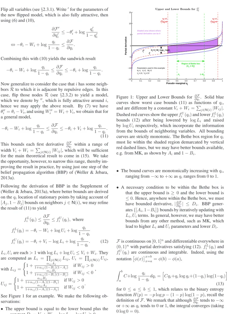
See Figure 1 for an example. We make the following ob-servations:
• The upper bound is equal to the lower bound plus the constantDi=Vi+Wi−logLi−logUi≥0.
0 0.1 0.2 0.3 0.4 0.5 0.6 0.7 0.8 0.9 1 −15 −10 −5 0 5 10 15
Upper and Lower Bounds for∂F ∂qi Pseudo−marginal qi Partial derivative fiU fiL Ai 1−Bi qi s.t. fiU(q i)=0 qi s.t. fiL(q i)=0
Region of Bethe box [Ai, 1−Bi] Di=Vi+Wi−logLi−logUi
Shaded area shows where partial derivative can be 0
Parameters used in this example:
θi=1, Vi=2, Wi=3 Li=1.8, Ui=2.9
Figure 1: Upper and Lower Bounds for ∂q∂F
i. Solid blue
curves show worst case bounds (11) as functions of qi,
and are different by a constantVi+Wi =Pj∈N(i)|Wij|.
Dashed red curves show the upperfU
i (qi)and lowerfiL(qi)
bounds (12) after being lowered by logLi and raised
by logUi respectively, which incorporate the information
from the bounds of neighboring variables. All bounding curves are strictly monotonic. The Bethe box region forqi
must lie within the shaded region demarcated by vertical red dashed lines, but we may have better bounds available, e.g. from MK, as shown byAiand1−Bi.
• The bound curves are monotonically increasing withqi,
ranging from−∞to+∞asqiranges from0to1.
• A necessary condition to be within the Bethe box is that the upper bound is≥ 0 and the lower bound is ≤0. Hence, anywhere within the Bethe box, we must have bounded derivative, |∂∂qF
i| ≤ Di. BBP
gener-ates{[Ai,1−Bi]}bounds by iteratively updating with
Li, Uiterms. In general, however, we may have better
bounds from any other method, such as MK, which lead to higherLiandUiparameters and lowerDi.
Fis continuous on[0,1]nand differentiable everywhere in
(0,1)nwith partial derivatives satisfying (12).fL
i (qi)and
fU
i (qi)are continuous and integrable. Indeed, using the
notationφ(x)x=b x=a=φ(b)−φ(a), Z b a C+log qi 1−qi dqi = h Cqi+qilogqi+(1−qi) log(1−qi) iqi=b qi=a (13) for0 ≤ a ≤ b ≤ 1, which relates to the binary entropy functionH(p) =−plogp−(1−p) log(1−p), recall the definition ofF. We remark that although∂∂qF
i tends to−∞
or+∞asqitends to0or1, the integral converges (taking
Hence ifqˆ= (ˆq1, . . . ,qˆn)is the location of a global
mini-mum, then for anyq= (q1, . . . , qn)in the Bethe box,
F(q)−F(ˆq)≤ X i:ˆqi≤qi Z qi ˆ qi fU i (qi)dqi+ X i:qi<qˆi Z qˆi qi −fL i (qi)dqi. (14) To construct a sufficient mesh, a simple initial bound relies on|∂∂qF
i| ≤ Di. If mesh pointsMi are chosen s.t. in
di-mensioni there must be a pointq∗ withinγi of a global minimum (which can be achieved using a mesh width in each dimension of2γi), then by settingγi = nDǫi, we
ob-tainF(q∗)− F(ˆq)≤P
iDinDǫi =ǫ. It is easily seen that
Ni ≤ 1 +⌈21γi⌉, hence the total number of mesh points,
N =P i∈VNi, satisfies N ≤2n+ n 2ǫ X i Di≤2n+n ǫ X (i,j)∈E |Wij| =O n ǫ X (i,j)∈E |Wij| =O nmW ǫ , (15) since Di ≤ Vi +Wi = Pj∈N(i)|Wij|. Here W =
max(i,j)∈E|Wij|andm=|E|is the number of edges.
If the initial model is fully attractive, then by Theo-rem 1 we obtain a submodular multi-label MAP problem which is solvable using graph cuts with worst case runtime O(N3) = O(ǫ−3n3m3W3)(Schlesinger & Flach, 2006;
Greig et al., 1989; Goldberg & Tarjan, 1988).
Note from the first expression in (15) that if we have in-formation on individual edge weights then we have a better bound usingP
(i,j)∈E|Wij|rather than justmW.
For comparison, the earlier second derivative approach of (Weller & Jebara, 2013a) has runtime O(ǫ−3
2n6Σ 3 4Ω
3 2), where, even using the improved method in§4 here,Ω = O(∆eW(1+∆/2)+T). Unlessǫis very small, the new first derivative approach is typically dramatically more efficient and more useful in practice. Further, it naturally handles both attractive and repulsive edge weights in the same way. 3.1 Refinements, adaptive methods
Since the resulting multi-label MAP inference problem is NP-hard in general (Shimony, 1994), it is helpful to min-imize its size. As noted above, setting γi = nDǫi, which
we term the simple method, yields a sufficient mesh, where |∂F
∂qi| ≤Di=Vi+Wi−logLi−logUi. However, since the
bounding curves are monotonic withfU
i ≥0andfiL ≤0,
a better bound for the magnitude of the derivative is often available by settingDi= max{fiU(1−Bi),−fiL(Ai)}.
3.1.1 The minsum method
We defineNi =the number of mesh points in dimension
i, with sumN = P
i∈VNi and productΠ =
Q
i∈VNi.
For a fully attractive model, the resulting MAP problem may be solved in timeO(N3)by graph cuts (Theorem 1,
(Schlesinger & Flach, 2006; Greig et al., 1989; Goldberg & Tarjan, 1988)), so it is sensible to minimizeN. In other cases, however, it is less clear what to minimize. For ex-ample, a brute force search over all points would take time Θ(Π).
Define the spread of possible values in dimensioniasSi=
1−Bi−Aiand noteNi= 1 +⌈2Sγii⌉is required to cover
the whole range. To minimizeNwhile ensuring the mesh is sufficient, consider the Lagrangian L = P
i∈V
Si
2γi −
λ(ǫ−P
i∈V γiDi), whereDiis set as in the simple method
(§3.1). Optimizing gives γi= ǫ P j∈V p SjDj r Si Di, withN≤2n+1 2ǫ X i∈V p SiDi !2 (16) which we term the minsum method. Note Di ≤ diW
wheredi is the degree ofXi, hence Pi∈V √SiDi
2 ≤ W P i∈V √ di 2
. By Cauchy-Schwartz and the handshake lemma, P i∈V √ di 2 ≤nP i∈Vdi = 2mn, with
equal-ity iff thediare constant, i.e. the graph is regular.
If insteadΠis minimized, rather than N, a similar argu-ment shows that the simple method (§3.1) is optimal. 3.1.2 Adaptive methods
The previous methods rely on one boundDifor|∂q∂Fi|over
the whole range[Ai,1−Bi]. However, we may increase
efficiency by using local bounds to vary the mesh width across the range. A bound on the maximum magnitude of the derivative over any sub-range may be found by check-ing just−fL
i at the lower end andfiU at the upper end.
This may be improved by using the exact integral as in (14). First, constant proportionski > 0 should be chosen with
P
iki = 1. Next, the first (lowest) mesh pointγ1i ∈ Mi
should be set s.t. Rγ1i
Aif
U
i (qi)dqi = kiǫ. This will ensure
thatγi
1covers all points to its left in the sense thatF[qi =
γi
1]− F[qi ∈ [Ai, γ1i]] ≤ kiǫ where all other variables
qj, j 6=i, are held constant at any values within the Bethe
box.γi
1also covers all points to its right up to what we term
its reach, i.e. the pointri
1s.t. Rri1 γi 1 −f L i (qi)dqi=kiǫ. Next,
γ2i is chosen as before, usingri1as the left extreme rather
thanAi, and so on, until the final mesh point is computed
with reach≥1−Bi. This yields an optimal mesh for the
choice of{ki}.
If ki = n1, we achieve an optimized adaptive simple
method. If ki = √S iDi P j∈V √ SjDj , we achieve an adaptive
minsum method. For many problems, this adaptive
min-sum method will be the most efficient.
knowl-edge, computing optimal points{γi
s} is not possible
ana-lytically, but each may be found with high accuracy in just a few iterations using a search method, hence total time to compute the mesh isO(N), which is negligible compared to solving the subsequent MAP problem.
4
REVISITING THE SECOND
DERIVATIVE APPROACH
We review the second derivative approach used in (Weller & Jebara, 2013a) (see§5 there). As here, the possible loca-tion of a global minimumqˆwas first bounded in the Bethe box given byQ
i∈V[Ai,1−Bi]. Next an upper boundΛ
was derived on the maximum possible eigenvalue of the Hessian H ofF anywhere within the Bethe box, where it was required that all edges be attractive. Then a mesh of constant width in every dimension was introduced s.t. the nearest mesh pointq∗toqˆwas at mostγaway in each dimension. Hence the ℓ2 distance δ satisfies δ2 ≤ nγ2
and by Taylor’s theorem,F(q∗) ≤ F(ˆq) + 1
2Λδ2.Λwas
computed by bounding the maximum magnitude of any el-ement ofH. Considering Theorem 7, this involves sepa-rate analysis of diagonalHiiterms, which are positive and
were bounded above by the term b; and edgeHij terms,
which are negative for attractive edges, whose magnitude was bounded above bya. ThenΩwas set asmax(a, b), andΣas the proportion of non-zero entries inH. Finally, Λ≤p
tr(HTH)≤√Σn2Ω2=nΩ√Σ.
4.1 Improved bound for an attractive model
We improve the upper bound for Λ by improving thea bound for attractive edges to derive˜a, a better upper bound on−Hij. Essentially, a more careful analysis allows a
po-tentially small term in the numerator and denominator to be canceled before bounding. Writingη¯= mini∈Vηi(1−ηi),
i.e. the closest that any dimension can come to 0 or 1, the result is that −Hij ≤ α ij 1 +αij , ¯ η 1− α ij 1 +αij 2! (17) = O(eW(1+∆/2)+T).
Thus, a˜ = O(eW(1+∆/2)+T) which compares favorably
to the earlier bound in (Weller & Jebara, 2013a) , where
a = O(eW(1+∆)+2T). Recall b = O(∆eW(1+∆/2)+T)
and Ω = max(a, b), so using the new ˜a bound, now Ω = O(∆eW(1+∆/2)+T). Details and derivation are in
the supplement.
4.2 Extending the second derivative approach to a general (non-attractive) model
Using flipping arguments from§2.3, we are able to extend the method of (Weller & Jebara, 2013a) to apply to general
models. Interestingly, the theoretical bounds derived for Ω = max(a, b)take exactly the same form as for the purely attractive case, except that now−W ≤Wij ≤W, whereas
previously it was required that0 ≤Wij ≤W. Since it is
a second derivative approach, the mesh size (measured by N, the total number of points summed over the dimensions) grows asO(ǫ−1/2)rather than asO(ǫ−1)in the new first
derivative approach. In practice, however, particularly for harder cases wherenandWare above small values, unless ǫ is very small, the method of§3 is much more efficient. Details and derivations are in the supplement.
5
RESULTING MULTI-LABEL MAP
After computing a sufficient mesh, it remains to solve the multi-label MAP inference problem on a MRF with the same topology as the initial model, where eachqitakes
val-ues inMi. In general, this is NP-hard (Shimony, 1994).
5.1 Tractable cases
If it happens that all cost functions are submodular (as is always the case if the initial model is fully attractive by Theorem 1), then as already noted, it may be solved effi-ciently using graph cut methods, which rely on solving a max flow/min cut problem on a related graph, with worst case runtime O(N3)(Schlesinger & Flach, 2006; Greig
et al., 1989; Goldberg & Tarjan, 1988). Using the Boykov-Kolmogorov algorithm (Boykov & Boykov-Kolmogorov, 2004), performance is typically much faster, sometimes approach-ingO(N). This submodular setting is the only known class of problem which is solvable for any topology.
Alternatively, the topological restriction of bounded tree-width allows tractable inference (Pearl, 1988). Further, un-der mild assumptions, this was shown to be the only re-striction which will allow efficient inference for any cost functions (Chandrasekaran et al., 2008). We note that if the problem has bounded tree-width, then so too does the original binary pairwise model, hence exact inference (to yield the true marginals or the true partition functionZ) on the original model is tractable, making our approximation result less interesting for this class. In contrast, although MAP inference is tractable for any attractive binary pair-wise model, marginal inference and computingZ are not (Jerrum & Sinclair, 1993).
A recent approach reducing MAP inference to identifying a maximum weight stable set in a derived weighted graph ((Jebara, 2013), (Weller & Jebara, 2013b)) shows promise, allowing efficient inference if the derived graph is perfect. Further, testing if this graph is perfect can be performed in polynomial time ((Jebara, 2013), (Chudnovsky et al., 2005)).
5.2 All other cases
Many different methods are available, see (Kappes et al., 2013) for a recent survey. Some, such as dual approaches, may provide a helpful bound even if the optimum is not found. Indeed, a LP relaxation will run in polynomial time and return an upper bound onlogZB that may be useful.
A lower bound may be found from any discrete point, and this may be improved using local search methods. Note also that BBP boundsqi ∈ [Ai,1−Bi]apply for all the
Bethe box, but for a particular value ofqisay, then the BBP
approach provides tighter bounds on each of its neighbors j ∈ N(i), which may be helpful for pruning the solution space.
5.2.1 Persistent partial optimization approaches MQPBO (Kohli et al., 2008) and Kovtun’s method (Kov-tun, 2003) are examples of this class. Both consider LP-relaxations and run in polynomial time. In our context, the output consists of ranges (which in the best case could be one point) of settings for some subset of the vari-ables. If any such ranges are returned, the strong per-sistence property ensures that any MAP solution satisfies the ranges. Hence, these may be used to update{Ai, Bi}
bounds (padding the discretized range to the full continu-ous range covered by the end points if needed), compute a new, smaller, sufficient mesh and repeat until no improve-ment is obtained.
6
EXPERIMENTS
As a first step toward applying our algorithm to explore the usefulness of the global optimum of the Bethe approx-imation, here we consider one setting where LBP fails to converge, yet still we achieve reasonable results.
We aim to predict transformer failures in a power network (Rudin et al., 2012). Since the real data is sensitive, our experiments use synthetic data. LetXi ∈ {0,1}indicate
if transformerihas failed or not. Each transformer has a probability of failure on its own which is represented by a singleton potential θi. However, when connected in a
network, a transformer can propagate its failure to nearby nodes (as in viral contagion) since the edges in the network form associative dependencies. We assume that homoge-neous attractive pairwise potentials couple all transformers that are connected by an edge, i.e. Wij =W ∀(i, j)∈ E.
The network topology creates a Markov random field spec-ifying the distributionp(X1, . . . , Xn). Our goal is to
com-pute the marginal probability of failure of each transformer within the network (not simply in isolation as in (Rudin et al., 2012)). Since recoveringp(Xi)is hard, we estimate
Bethe pseudo-marginalsqi=q(Xi= 1)through our
algo-rithm, which emerge as the arg minwhen optimizing the Bethe free energy.
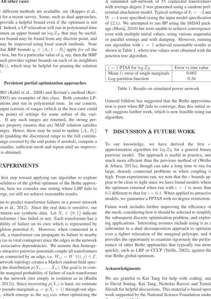
A simulated sub-network of 55 connected transformers with average degree 2 was generated using a random pref-erential attachment model. Typical settings ofθi =−2and
W = 4were specified (using the input model specification of§2.1). We attempted to run BP using the libDAI pack-age (Mooij, 2010) but were unable to achieve convergence, even with multiple initial values, using various sequential or parallel settings and with damping. However, running our algorithm with ǫ = 1achieved reasonable results as shown in Table 1, where true values were obtained with the junction tree algorithm.
ǫ= 1PTAS forlogZB Error vs true value
Meanℓ1error of single marginals 0.003
Log-partition function 0.26 Table 1: Results on simulated power network General folklore has suggested that the Bethe approxima-tion is poor when BP fails to converge, thus this initial re-sult suggests further work, which is now feasible using our algorithm.
7
DISCUSSION & FUTURE WORK
To our knowledge, we have derived the first ǫ -approximation algorithm for logZB for a general binary
pairwise model. The approach is useful in practice, and much more efficient than the previous method of (Weller & Jebara, 2013a), though can take a long time to run for large, densely connected problems or when coupling is high. From experiments run, we note that theǫbounds ap-pear to be close to tight since we have found models where the optimum returned when run with ǫ = 1is more than 0.5different to that forǫ= 0.1. When applied to attractive models, we guarantee a FPTAS with no degree restriction. Future work includes further improving the efficiency of the mesh, considering how it should be selected to simplify the subsequent discrete optimization problem, and explor-ing applications. Interestexplor-ing avenues include usexplor-ing it as a subroutine in a dual decomposition approach to optimize over a tighter relaxation of the marginal polytope, and it provides the opportunity to examine rigorously the perfor-mance of other Bethe approaches that typically run more quickly, such as LBP or CCCP (Yuille, 2002), against the true Bethe global optimum.
Acknowledgments
We are grateful to Kui Tang for help with coding, and to David Sontag, Kui Tang, Nicholas Ruozzi and Toma˘z Slivnik for helpful discussions. This material is based upon work supported by the National Science Foundation under Grant No. 1117631.
References
Abdelbar, A., & Hedetniemi, S. (1998). Approximating MAPs for belief networks is NP-hard and other theo-rems. Artificial Intelligence, 102, 21–38.
Alon, N., & Tarsi, M. (1985). Covering multigraphs by simple circuits. SIAM Journal on Algebraic Discrete
Methods, 6, 345–350.
Bethe, H. (1935). Statistical theory of superlattices. Proc.
R. Soc. Lond. A, 150, 552–575.
Boykov, Y., & Kolmogorov, V. (2004). An experimental comparison of min-cut/max-flow algorithms for energy minimization in vision. IEEE Trans. Pattern Anal. Mach.
Intell., 26, 1124–1137.
Chandrasekaran, V., Chertkov, M., Gamarnik, D., Shah, D., & Shin, J. (2011). Counting independent sets using the Bethe approximation. SIAM J. Discrete Math., 25, 1012– 1034.
Chandrasekaran, V., Srebro, N., & Harsha, P. (2008). Com-plexity of inference in graphical models. UAI (pp. 70– 78). AUAI Press.
Chudnovsky, M., Cornu´ejols, G., Liu, X., Seymour, P., & Vuskovic, K. (2005). Recognizing Berge graphs.
Com-binatorica, 25, 143–186.
Cooper, G. (1990). The computational complexity of prob-abilistic inference using Bayesian belief networks.
Arti-ficial Intelligence, 42, 393–405.
Daskalakis, C., & Papadimitriou, C. (2011). Continuous local search. Proceedings of ACM-SIAM Symposium on
Discrete Algorithms (SODA) (pp. 790–804).
Goldberg, A., & Tarjan, R. (1988). A new approach to the maximum flow problem. Journal of the ACM, 35, 921– 940.
Greig, D., Porteous, B., & Seheult, A. (1989). Exact maxi-mum a posteriori estimation for binary images. J. Royal
Statistical Soc., Series B, 51, 271–279.
Gurvits, L. (2011). Unleashing the power of Schrijver’s permanental inequality with the help of the Bethe ap-proximation. Elec. Coll. Comp. Compl.
Hazan, T., & Jaakkola, T. (2012). On the partition function and random maximum a-posteriori perturbations. ICML. Heinemann, U., & Globerson, A. (2011). What cannot be learned with Bethe approximations. UAI (pp. 319–326). Heskes, T. (2004). On the uniqueness of loopy belief prop-agation fixed points. Neural Computation, 16, 2379– 2413.
Huang, B., & Jebara, T. (2009). Approximating the
perma-nent with belief propagation (Technical Report).
Jebara, T. (2013). Tractability: Practical approaches to
hard problems, chapter Perfect graphs and graphical
modeling. Cambridge Press.
Jerrum, M., & Sinclair, A. (1993). Polynomial-time ap-proximation algorithms for the Ising model. SIAM J.
Comput., 22, 1087–1116.
Kappes, J., Andres, B., Hamprecht, F., Schn ¨orr, C., Nowozin, S., Batra, D., Kim, S., Kausler, B., Lellmann, J., Komodakis, N., & Rother, C. (2013). A comparative study of modern inference techniques for discrete energy minimization problems. CVPR.
Kohli, P., Shekhovtsov, A., Rother, C., Kolmogorov, V., & Torr, P. (2008). On partial optimality in multi-label MRFs. ICML (pp. 480–487). ACM.
Korc, F., Kolmogorov, V., & Lampert, C. (2012).
Approx-imating marginals using discrete energy minimization
(Technical Report). IST Austria.
Kovtun, I. (2003). Partial optimal labeling search for a NP-hard subclass of (max, +) problems. DAGM-Symposium (pp. 402–409). Springer.
McEliece, R., MacKay, D., & Cheng, J. (1998). Turbo decoding as an instance of Pearl’s ”Belief Propagation” algorithm. IEEE Journal on Selected Areas in
Commu-nications, 16, 140–152.
Mooij, J. (2010). libDAI: A free and open source C++ library for discrete approximate inference in graphical models. Journal of Machine Learning Research, 11,
2169–2173.
Mooij, J., & Kappen, H. (2007). Sufficient conditions for convergence of the sum-product algorithm. IEEE
Trans-actions on Information Theory, 53, 4422–4437.
Murphy, K., Weiss, Y., & Jordan, M. (1999). Loopy be-lief propagation for approximate inference: An empir-ical study. Proceedings of the Fifteenth conference on
Uncertainty in artificial intelligence (pp. 467–475).
Pearl, J. (1988). Probabilistic reasoning in intelligent
sys-tems: Networks of plausible inference. Morgan
Kauf-mann.
Peierls, R., & Born, M. (1936). On Ising’s model of ferro-magnetism. Proc. Camb. Phil. Soc., 32, 477.
Pletscher, P., & Kohli, P. (2012). Learning low-order mod-els for enforcing high-order statistics. Artificial
Rudin, C., Waltz, D., Anderson, R., Boulanger, A., Salleb-Aouissi, A., Chow, M., Dutta, H., Gross, P., Huang, B., & Ierome, S. (2012). Machine learning for the New York City power grid. IEEE Trans. Pattern Anal. Mach. Intell.,
34, 328–345.
Ruozzi, N. (2012). The Bethe partition function of log-supermodular graphical models. Neural Information Processing Systems.
Schlesinger, D., & Flach, B. (2006). Transforming an
arbi-trary minsum problem into a binary one (Technical
Re-port). Dresden University of Technology.
Shimony, S. (1994). Finding MAPs for belief networks is NP-hard. Aritifical Intelligence, 68, 399–410.
Shin, J. (2012). Complexity of Bethe approximation.
Arti-ficial Intelligence and Statistics.
Shin, J. (2013). The complexity of approximating a Bethe equilibrium. CoRR, abs/1109.1724.
Teh, Y., & Welling, M. (2002). The unified propagation and scaling algorithm. Advances in Neural Information
Processing Systems.
Valiant, L. (1979). The complexity of computing the per-manent. Theoretical Computer Science, 8, 189–201. Vontobel, P. (2010). The Bethe permanent of a
non-negative matrix. Communication, Control, and
Comput-ing (Allerton), 2010 48th Annual Allerton Conference on
(pp. 341–346).
Wainwright, M., & Jordan, M. (2008). Graphical models, exponential families and variational inference.
Founda-tions and Trends in Machine Learning, 1, 1–305.
Watanabe, Y. (2011). Uniqueness of belief propagation on signed graphs. Neural Information Processing Systems. Watanabe, Y., & Chertkov, M. (2010). Belief propagation
and loop calculus for the permanent of a non-negative matrix. Journal of Physics A: Mathematical and
Theo-retical, 43, 242002.
Weller, A., & Jebara, T. (2013a). Bethe bounds and ap-proximating the global optimum. Artificial Intelligence
and Statistics.
Weller, A., & Jebara, T. (2013b). On MAP inference by MWSS on perfect graphs. Twenty Ninth Conference on
Uncertainty in Artificial Intelligence (UAI).
Welling, M., & Teh, Y. (2001). Belief optimization for bi-nary networks: A stable alternative to loopy belief prop-agation. Uncertainty in Artificial Intelligence.
Yedidia, J., Freeman, W., & Weiss, Y. (2001). Understand-ing belief propagation and its generalizations.
Interna-tional Joint Conference on Artificial Intelligence, Distin-guished Lecture Track.
Yuille, A. (2002). CCCP algorithms to minimize the Bethe and Kikuchi free energies: Convergent alternatives to be-lief propagation. Neural Computation, 14, 1691–1722.
APPENDIX: SUPPLEMENTARY MATERIAL FOR APPROXIMATING THE BETHE
PARTITION FUNCTION
Here we provide further details and proofs of several of the results in the main paper, using the original numbering.
4
REVISITING THE SECOND DERIVATIVE APPROACH
4.1 Improved bound for an attractive model
In this section, we improve the upper bound for Λ by improving thea bound for attractive edges to derivea˜, an im-proved upper bound on−Hij. Essentially, a more careful analysis allows a potentially small term in the numerator and
denominator to be canceled before bounding. Using Theorem 7, equation (9) and Lemma 5,
−Hij = (ξij−qiqj) 1 Tij ≤m(11 +−Mα)αij ij 1 m(1−M) (1−m)M −m(1−M) αij 1+αij 2 = α ij 1 +αij 1 (1−m)M−m(1−M) αij 1+αij 2 (18)
wherem= min(qi, qj), M = max(qi, qj). Now we use the following result.
Lemma 8. For anyk∈(0,1), lety= minqi∈[Ai,1−Bi],qj∈[Aj,1−Bj](1−m)M−m(1−M)k, then
y= BiAj−(1−Bi)(1−Aj)k if(1−Bi)≤Aj i range≤j range
(1−k) min{Aj(1−Aj), Bi(1−Bi)} ifAi≤Aj ≤1−Bi ≤1−Bj ranges overlap, i lower
(1−k) min{Aj(1−Aj), Bj(1−Bj)} ifAi≤Aj ≤1−Bj ≤1−Bi j range⊆i range
(1−k) min{Ai(1−Ai), Bi(1−Bi)} ifAj ≤Ai ≤1−Bi ≤1−Bj i range⊆j range
(1−k) min{Ai(1−Ai), Bj(1−Bj)} ifAj ≤Ai ≤1−Bj ≤1−Bi ranges overlap, j lower
BjAi−(1−Bj)(1−Ai)k if(1−Bj)≤Ai j range ≤i range.
Proof. The minimum is achieved by minimizing the larger and maximizing the smaller ofqiandqj. The result follows for
cases where their ranges are disjoint. If ranges overlap, then the minimum is achieved at someqi=qjin the overlap, with
valueqi(1−qi)(1−k), which is concave and minimized at an extreme of the overlap range.
Lemma 8 is useful in practice, and should be used to compute ˜a = max(i,j)∈E of the bound above. To analyze the theoretical worst case, it is straightforward to see the corollary thaty ≥ (1−k)¯η, whereη¯ = mini∈Vηi(1−ηi). This
bound can be met, for example, if all ranges coincide. Hence, from (18), and with the reasoning for 1¯η from (Weller & Jebara, 2013a)§5.3, where it is shown thatηi(11
−ηi) =O(eT+∆W/2), and usingαij =eWij −1, we obtain
−Hij ≤ αij 1 +αij , ¯ η 1− αij 1 +αij 2! =O(eW(1+∆/2)+T). (19)
Thus, a˜ = O(eW(1+∆/2)+T) which compares favorably to the earlier bound in (Weller & Jebara, 2013a) , where
a = O(eW(1+∆)+2T). Recall b = O(∆eW(1+∆/2)+T) and Ω = max(a, b), so using the new a˜ bound, now
4.2 Extending the second derivative approach to a general (non-attractive) model
Here we extend the analysis of (Weller & Jebara, 2013a) by considering repulsive edges to show that for a general binary pairwise model, we can still calculate useful bounds (which turn out to be very similar to the earlier bounds for attractive models) for a sufficient mesh width.
Our main tool for dealing with a repulsive edge is to flip the variable at one end (see§2.3) to yield an attractive edge, then we can apply earlier results. We denote the flipped model parameters with a′. For example, if just variableXjis flipped,
thenq′
j =q(Xj′ = 1) =q(1−Xj= 1) = 1−qj. Sinceαij =eWij−1and hereWij′ =−Wij, the following relationship
holds if one end of an edge is flipped, α′ ij 1 +α′ ij = e− Wij −1 e−Wij = 1−e Wij =−α ij. (20)
Note that, for an attractive edge, α
′
ij 1+α′
ij ∈ (0,1), as is−αij
for a repulsive edge. Recall that when we flip some set of variables, by constructionF′=F+constant(see§2.3).
The Hessian terms from Theorem 7 still apply. Our goal is to bound the magnitude of each entryHijfor a general binary
pairwise model, then the earlier analysis will provide the result. Whereas for a fully attractive model, we assumed a maximum edge weightW with0≤Wij ≤W, now we assume|Wij| ≤W.
4.2.1 Edge terms
First considerHij for an edge(i, j)∈ E. If the edge is attractive, then the earlier analysis holds (it makes no difference
if other edges are attractive or repulsive). If it is repulsive, thenHij > 0. Consider a model where justXj is flipped.
Hij = ∂ 2 F ∂qi∂qj = − ∂2 F′ ∂q′ i∂q ′ j = −H ′
ij. Hence using (18) and (20), in practice an upper bound may be computed from
Lemma 8 usingk = −αij andA′j = Bj, B′j = Aj. The theoretical bound for an attractive edge from (19) becomes
Hij ≤η¯(1−−ααij2
ij)
. As we should expect from the attractive case, the following result holds. Lemma 9. For a repulsive edge, 1 1
−α2
ij =O(e
−Wij).
Proof. Letu=−Wij, thenαij =e−u−1and1−1α2
ij =
1
(1−αij)(1+αij) = 1
e−u(2−e−u) =O(eu).
Hence, noting that we may flip any neighbors j of i which are adjacent via repulsive edges to obtain ηi(11 −ηi) =
O(eT+∆W/2)as before, where nowW = max
(i,j)∈E|Wij|, we see that for our new second derivative method, just as
in the fully attractive case,˜a=O(eW(1+∆/2)+T).
For comparison interest, we also show how the earlier, worse bound for an attractive edge given in (Weller & Jebara, 2013a) may similarly be combined with flipping to provide a worse upper bound forHij when(i, j)is repulsive. See (Weller &
Jebara, 2013a)§5.2: considering the proof of Lemma 10 and using (20) from this paper, we see that for a repulsive edge, the Kij minimum bound forTij becomesKij = ηiηj(1−ηi)(1−ηj)(1−α2ij); then from (Weller & Jebara, 2013a)
Theorem 11, the equivalent bound isHij ≤−4Kαijij which givesa=O(eW(1+∆)+2T)as it was for the fully attractive case.
We provide a further interesting result, deriving a lower bound forξijfor a repulsive edge.
Lemma 10 (Lower bound forξijfor a repulsive edge, analogue of Lemma 5). For any repulsive edge(i, j),
qiqj−ξij≤ −αijpijwherepij = min{qiqj,(1−qi)(1−qj)}.
Proof. Consider a model where just variable Xj is flipped, and let all new quantities be designated by the symbol′.
Consider the joint pseudo-marginal (3). In the new model the columns are switched sinceµ′
ij(a, b) =q(Xi′ =a, Xj′ = b) =q(Xi=a, Xj= 1−b) =µij(a,1−b), hence µ′ ij = 1 +ξ′ ij−q′i−q′j qj′ −ξij′ q′ i−ξ′ij ξij′ = qj−ξij 1 +ξij−qi−qj ξij qi−ξij . (21)
Applying Lemma 5 to the new model,ξ′
ij−q′iqj′ ≤ α′ ij 1+α′ ijm ′(1−M′). Substituting inξ′
ij =qi−ξijfrom (21) and using
(20), we have(qi−ξij)−qi(1−qj)≤ −αijm′(1−M′). Sincem′= min{qi,1−qj}andM′ = max{qi,1−qj}, noting
Hence for a repulsive edge(i, j), using (9), we have
Tij=qiqj(1−qi)(1−qj)−(ξij−qiqj)2≥pijPij−α2ijp2ij,
wherePij = max{qiqj,(1−qi)(1−qj)}.
4.2.2 Diagonal terms
Consider theHiiterms from Theorem 7, which is true for a general model. If all neighbors ofXiare adjacent via attractive
edges, then, as in (Weller & Jebara, 2013a) Theorem 11,Hii≤ ηi(11−ηi) 1−di+Pj∈N(i) 1 1−1+αij
αij
2
!
.
If any neighbors are connected toXiby a repulsive edge, then consider a new model where those neighbors are flipped,
so now all edges incident to Xi are attractive, and designate the new model parameters with a ′. As before, observe
F =F′+constant, henceHii= ∂2 F ∂q2 i = ∂2 F′ ∂q′2 i =H ′
ii. Using (20) we obtain that for a general model,
Hii ≤ 1 ηi(1−ηi) 1−di+ X j∈N(i):Wij>0 1 1− αij 1+αij 2+ X j∈N(i):Wij<0 1 1−α2 ij . (22)
Similarly to the analysis in§4.2.1, using Lemma 9 gives that for a general model,b= maxi∈VHii=O(∆eW(1+∆/2)+T),