Grid Multi-classification Adaptive Classification Testing with Multidimensional Polytomous Items

(1)

Grid Multi-classification Adaptive Classification Testing

with Multidimensional Polytomous Items

A THESIS

SUBMITTED TO THE FACULTY OF THE UNIVERSITY OF MINNESOTA

BY

Zhuoran Wang

IN PARTIAL FULFILLMENT OF THE REQUIREMENTS FOR THE DEGREE OF

DOCTOR OF PHILOSOPHY

Advisor: Chun Wang Co-Advisor: Niels Waller

(2)

© Zhuoran Wang 2019

(3)

i Acknowledgements

There are many people that have earned my gratitude for their contribution to my time in graduate school. The following is only an incomplete list of those I have met along the way.

Firstly, I would like to express my sincere gratitude to my advisor Dr. Chun Wang for the continuous support of my Ph.D. study and related research, for her patience, motivation, and immense knowledge. Her guidance helped me in all the time of research and writing of this thesis. I could not have imagined having a better advisor and mentor for my Ph.D. study.

In addition to my advisor, I would like to thank the rest of my thesis committee: Dr. David Weiss, Dr. Niels Waller, and Dr. Mark Davison, for their insightful comments and encouragement, but also for their thought-provoking courses and support on my multiple course projects.

I thank my colleagues on the sixth floor of Elliott Hall, Lauren Berry, Allie Cooperman, Kayle Donner, Leah Feuerstahler, Shengyu Jiang, Justin Kracht, Hoang Nguyen, Alec Nyce, Chaitali Phadke, Gretchen Saunders, Matthew Snodgress, King Yiu Suen, and Ziming Zhou, for the stimulating discussions and for all the fun we have had in the last five years.

(4)

ii Last but not least, I would like to express my deepest gratitude to my family and friends. This thesis would not have been possible without their warm love, continued patience, and endless support.

This research was supported by the Eunice Kennedy Shriver National Institutes of Child Health and Human Development of the National Institutes of Health under Award Number R01HD079439 to the Mayo Clinic in Rochester Minnesota through subcontracts to the University of Minnesota and the University of Washington. The content is solely the responsibility of the author and does not necessarily represent the official views of the National Institutes of Health.

(5)

iii

Abstract

Adaptive classification testing (ACT) is a form of computerized adaptive testing (CAT) that was developed to efficiently classify examinees into multiple categories based on predetermined classification cutoff scores. All existing multidimensional ACT studies handle multidimensional classifications in a unidimensional space by performing

classification on a composite of multiple traits. However, classification along separate dimensions is sometimes preferred because it provides clearer information regarding a person’s relative standing along each dimension. This type of classification is referred to as grid classification, as each examinee is classified into one of the grids encircled by cutoff scores (lines/surfaces) on different dimensions. Complications arise when there is more than one cutoff score along each dimension. In order to perform grid classification using ACT, two termination criteria, sequential probability ratio test (SPRT) and

confidence interval (CI) were adopted from one-dimensional classification in the between-item multidimensional test. In addition, two new termination criteria for grid multi-classification ACT were developed, namely, grid classification generalized

likelihood ratio (GGLR) and simplified generalized likelihood ratio (SGLR). A new item selection rule, i.e., posterior weighted D-optimal on cutoff points (PWCD-optimal), was also proposed.

Three simulation studies were conducted to evaluate the performance of ACT for multidimensional grid classification. The three-dimensional multidimensional graded response model (MGRM) with four response categories was used. The item bank contained 300 between-item multidimensional items with 100 items loading on each

(6)

iv dimension. Examinees were classified into four groups along each dimension, resulting in

43 = 64 classification grids in total. The minimum and maximum test length were fixed at 7 and 60 items. Three item selection methods (D-optimal, PWCD-optimal, and

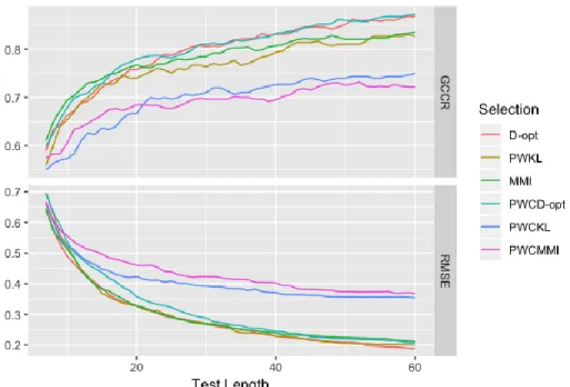
multidimensional mutual information (MMI)) and four termination criteria (GGLR, SGLR, CI, and SPRT) were applied in the grid multi-classification ACT.

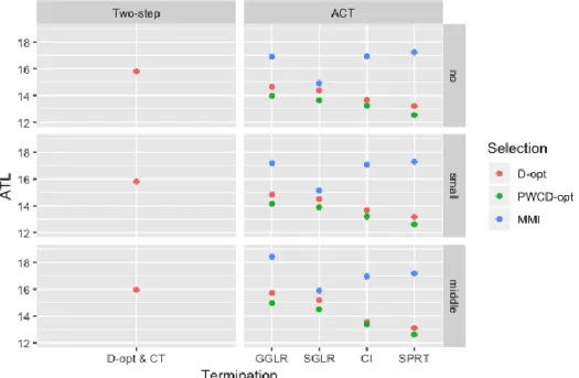
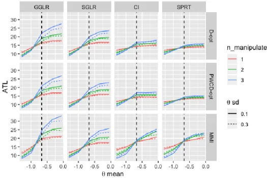
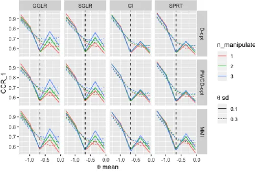
The first study compared ACT to the two-step measurement CAT-based classification. In the latter scenario, a variable-length multidimensional CAT was conducted, followed by a post-hoc classification. The D-optimal item selection method and the compound termination criteria were used in the two-step approach. The cutoffs for each termination criterion in the two approaches were selected to carefully yield similar classification accuracy, such that the resulting average test length (ATL) was a useful indicator of test efficiency. Results showed that, when D-optimal and PWCD-optimal item selection methods were used, ACT resulted in up to 20% shorter ATLs than the two-step approach. In this way, ACT was more efficient than the two-step approach. Among the four termination criteria for ACT, SPRT, and CI outperformed the two new termination criteria.

The second study further explored the influence of true latent trait location on classification accuracy and test length using grid multi-classification ACT. Instead of simulating discrete 𝛉points, 𝛉distributions with various mean vectors and variance-covariance matrices were used to represent true latent traits at different locations. One, two, or three dimensions were manipulated. For the manipulated dimensions, six 𝜃 mean levels and two 𝜃 standard deviation levels were considered. Generally, classification was

(7)

v more difficult when examinees were closer to the cutoff scores. PWCoptimal and D-optimal lead to stable test length and classification accuracy. As SPRT and CI resulted in lower classification accuracy for examinees that were close to the cutoff points, thus were difficult to be classified, the overall high efficiency of SPRT and CI in Study 1 can be largely attributed to the large proportion of examinees that were far from the cutoff points in the normally distributed population. As stable classification accuracy across 𝛉

distribution is generally desired in ACT, SGLR and GGLR were found to be preferable. The third study utilized real item parameters from a health measurement bank containing 324 Likert-scale items and 366 real examinee parameters to compare the performance of ACT and the two-step measurement CAT-based approach in terms of grid classification. Due to the influence of item bank quality, the test lengths were much longer than those in Study 1. All the conditions using MMI resulted in test length longer than the maximum test length (60 items). When D-optimal and PWCD-optimal item selection methods were used, ACT still outperformed the two-step approach and saved up to 20% of items as in Study 1. However, the superiority of PWCD-optimal did not always hold. CI and SPRT still led to shorter ATL than the other two termination criteria.

(8)

vi

List of Tables

Table 1. The two-step approach and ACT classification efficiency ... 78 Table 2. Latent trait distributions ... 87

(14)

xii

List of Figures

Figure 1. Multi-classification GLR ... 26

Figure 2. Relevant cutoff points ... 37

Figure 3. GGLR for grid classification ... 38

Figure 4. SGLR for grid classification ... 39

Figure 5. Possible standard error by fixing 𝜃2 and 𝜃3 to 0 ... 69

Figure 6. Classification and estimation accuracy with varying item selection methods . 71 Figure 7. Classification and estimation accuracy with varying number of quadrature points ... 73

Figure 8. Average test length with varying item selection methods and termination criteria ... 80

Figure 9. Determinant of item bank Fisher information by fixing 𝜃2 and 𝜃3 to 0 ... 83

Figure 10. Determinant of possible test Fisher information by fixing 𝜃2 and 𝜃3 to 0 .... 84

Figure 11. Average test length with varying item selection methods, termination criteria, 𝜃 mean, 𝜃 standard deviation, and number of manipulated dimensions ... 90

Figure 12. CCR of dimension 1 with varying item selection methods, termination criteria, 𝜃 mean, 𝜃 standard deviation, and number of manipulated dimensions ... 91

Figure 13.CCR of dimension 2 with varying item selection methods, termination criteria, 𝜃 mean, 𝜃 standard deviation, and number of manipulated dimensions ... 92

Figure 14. CCR of dimension 3 with varying item selection methods, termination criteria, 𝜃 mean, 𝜃 standard deviation, and number of manipulated dimensions ... 93

(15)

xiii

Figure 16. Ability distribution on each dimension of the real examinees ... 99 Figure 17. Average test length with varying item selection methods and termination criteria ... 101

(16)

1

1. Introduction

Classification testing refers to the family of tests in which examinees are

classified into two or more groups based on predetermined classification cutoff points. A classification test determines whether an examinee meets the requirement for a particular purpose (Norcini & Guille, 2002). If the goal of a test is to classify people, it is

unnecessary to obtain very precise ability/latent trait estimate on a continuous scale. Instead, the coarser-grained classification testing is more efficient. Classification testing is widely used in educational (Eggen & Straetmans, 2000), occupational, and medical (Smits & Finkelman, 2013) areas. For example, it is common to classify examinees into multiple fluency levels in the language testing domain. Interagency Language Roundtable uses 0, 0+, 1, …, 3 to characterize spoken-language use. Occupational certificate and license tests essentially categorize examinees into passing or failing groups, then grant the passing group the corresponding certificate or license. Clinical questionnaires also classify examinees. Beck’s Depression Inventory classifies examinees from “These ups and downs are considered normal” to “Extreme depression”. Classification testing further facilitates subsequent treatment (after clinic diagnosis) or teaching (after competence-based class grouping). Within the treatment, multiple participants can work together to promote treatment as well as provide more targeted feedback for the plan to improve (Welch & Frick, 1993).

To administer the classification test in a more efficient manner, computerized adaptive testing (CAT) can be adopted as the testing format. CAT has gained great

(17)

2 popularity because it shortens test length while maintaining high precision of ability estimates. To avoid ambiguity, in this thesis, CAT integrated with classification testing is called Adaptive Classification Testing (ACT), whereas CAT used to accurately estimate examinees’ abilities is referred to as measurement CAT. Measurement CAT can also be used for classification purpose. After it is stopped by either precision-related termination criteria or fixed test length, the ability estimate is compared to the predetermined cutoff point so as to arrive at a classification result. This is a two-step procedure, while ACT directly arrives at the classification decision. The advantage brought by adaptive algorithms tends to be even more compelling in ACT than in the measurement CAT-based two-step approach (referred to as two-step approach in the rest of this thesis), as the examinees, who are located far from the cutoff points, can be classified with a few items and relatively rough ability estimate. In these cases, ACT can sometimes be cut short. In order to reach the same level of classification accuracy, test lengths vary among

examinees. That is, variable-length tests can fully exert the advantage of adaptiveness in classification testing. Hence, the ACTs are of variable length. Lewis and Sheehan (1990) found that ACT reduced the test length up to 50% on average without sacrificing

classification accuracy.

Dimensionality is an unavoidable issue in the testing area. Traits are essentially associated, thus some of the tests are, by nature, multidimensional through using items measuring multiple traits. Furthermore, combining several unidimensional tests

measuring different dimensions takes advantage of the information brought by other dimensions, thus it should result in a more accurate ability estimate or higher

(18)

3 classification accuracy than using multiple unidimensional tests separately (Frey & Seitz, 2009; Seitz & Frey, 2013; Luecht, 1996; Segall, 1996). As a result, multidimensional testing has gained great popularity recently. This trend is also true in ACT, reflected by the increasing number of studies on multidimensional ACT (van Groen, 2014; van Groen, Eggen, & Veldkamp, 2016; Nydick, 2013; Seitz & Frey, 2013). However, all of the existing multidimensional ACT studies simplify the multidimensional classification problems to unidimensional ones, hence classification explicitly on each dimension is not viable. On the other hand, classification on each of the original dimensions has more practical meaning and can provide guidance to the following treatment and teaching. This kind of cross- classification in multidimensional classification testing is named grid classification in this thesis, as examinees are classified into one of the grids encircled by cutoff scores (lines/surfaces) on different dimensions.

Moreover, the number of categories also has a sizeable influence on the

classification procedure. ACT started as mastery testing, which classifies examinees into only two categories: master and non-master, or pass and fail (Lewis & Sheehan, 1990; Spray et al., 1997; Weiss & Kingsbury, 1984). Occupational certification testing often employs this kind of ACT. Later on, multi-classification tests (examinees are classified into more than two categories) emerged in areas such as language testing and physical evaluations (Glas & Vos, 2009; van Groen, 2014; van Groen, Eggen, & Veldkamp, 2014; Seitz & Frey, 2013). The majority of the recent ACT studies focus on mastery testing, while ignoring the more general, yet more complicated multi-classification cases.

(19)

4 Last but not least, polytomous items need to be promoted in ACT construction. Polytomous items have been broadly used in a variety of exams due to the prevalence of Likert- scale items and partial credit items. In addition, there are several strengths from a psychometric perspective. One of these strengths is that polytomous items provide more information than dichotomous items over a wider range (Samejima, 1976; Birenbaum & Tatsuoka, 1987; Donoghue, 1994). In this way, polytomous items could reduce the test length, while achieving the same effects as dichotomous items, particularly under a CAT context (De Ayala, 1989; De Ayala, Dodd, & Koch, 1992). An additional benefit is that item exposure is rather balanced even without deliberate control (van Rijin et at., 2002). It is also believed that polytomous items measure concepts and skills at greater depth than dichotomous items (Ercikan et al., 1998). However, polytomous items are underused in ACT (Smits & Finkelman, 2013; Thompson, 2007) and they have never been used in multidimensional ACT.

In order to address the above issues and enrich the multidimensional ACT research literature, this thesis focuses on designing efficient multidimensional multi-classification ACT with polytomous items. From a practical point of view, tests entailing items measuring exactly one dimension each (between-item multidimensionality) are much more common than tests based on an item pool with within-item

multidimensionality (Seitz & Frey, 2013). Thus, this thesis only addresses ACT with between-item multidimensionality. In the following sections, the prevalent IRT models as well as the current literatures on ACT item selection methods and termination criteria are reviewed. A few new item selection methods and termination criteria, specifically

(20)

5 developed for the grid multi-classification ACT, using polytomous items are proposed. Finally, three simulation studies are implemented to compare ACT to the two-step approach, in terms of classification efficiency, as well as evaluate the performance of item selection methods and termination criteria in ACT.

(21)

6

2. IRT Models in ACT

Selecting an appropriate IRT model for the data is an important precondition of ACT administration. Please note, ACT and measurement CAT can share the same IRT model as well as the item bank. Thus, the models listed below can be used in both ACT and the two-step approach. As a large proportion of ACT studies were conducted using unidimensional models and multidimensional dichotomous models, all these models as well as multidimensional polytomous models, which are the core of this thesis, are reviewed here.

2.1 Unidimensional Models

The most popular unidimensional IRT model is the three-parameter logistic (3PL) model (Birnbaum, 1968). Its popularity spans across both linear testing (all examinees respond to the same test irrespective of their latent trait levels) and adaptive testing, and both measurement CAT and ACT (Lin & Spray, 2000; Thompson & Ro, 2007;

Weissman, 2007; Bartroff, Finkelman, & Lai, 2008; Thompson, 2010; Lin, 2011). It is a dichotomous model. That is, for each item there are only two scoring options: 1 and 0, indicating correct and incorrect. The probability of examinee 𝑖 correctly responding to item 𝑗 is

𝑃_𝑗(𝜃𝑖) = 𝑐𝑗+

1 − 𝑐_𝑗

(22)

7 where 𝜃_𝑖 is the ability of examinee 𝑖. As this study focuses on adaptive testing, each examinee is assumed to finish the test independently. From here on, the examinee index 𝑖

is dropped. 𝑎𝑗, 𝑏𝑗 and 𝑐𝑗 are the discrimination, difficulty, and pseudo-guessing parameters of item 𝑗, respectively. When 𝑐𝑗 = 0, the 3PL model becomes the two-parameter logistic (2PL) model. 2PL model is also used in numerous ACT studies (Eggen, 1999, 2009; Eggen & Straetmans, 2000; Wonda & Eggen, 2009). Moreover, when the 𝑎_𝑗s are equal across the entire test, the one-parameter logistic (1PL) model is obtained.

Different from dichotomous IRT models, polytomous IRT models are scored on more than two options, from 1 to 𝑅 (𝑅 > 2). Generally, polytomous items provide wider-spread and higher item information which potentially can shorten the test length in ACT and measurement CAT while keeping accurate classification and estimation. The

conventional polytomous IRT models include the partial credit model (PCM; Master, 1982), the graded response model (GRM) (Samejima, 1968), the generalized partial credit model (GPCM; Muraki, 1992), the nominal response model (NRM; Bock, 1972) and the rating scale model (RSM; Andrich, 1978; Muraki, 1990). Although all

polytomous models can deal with the same format of responses, they have different assumptions about the response process. According to Dodd, De Ayala, and Koch (1995), the GRM, GPCM, and PCM can be adopted for data ordered to represent various degrees of the latent trait measure. The PCM model is specifically fit for items in mathematics, physics, and chemistry because points are awarded for the completion of steps leading to the correct answer. The GPCM is a similar version of the PCM model with the exception

(23)

8 of having varying slope parameters in different items. The GRM model is frequently used in analyzing Likert-scale item responses. As both the GPCM and GRM models have been used in ACT studies (Lau & Wang, 1998, 1999; Thompson, 2007; Gnambs & Batinic, 2011; Smits & Finkelman, 2013), they are reviewed in detail.

The GPCM model is formulated on the assumption that the probability of

choosing option 𝑟 over option 𝑟 − 1 in item 𝑗 is governed by the logistic response model

𝐶𝑗𝑟 =

𝑃_𝑗𝑟(𝜃) 𝑃𝑗,𝑟−1(𝜃) + 𝑃𝑗𝑟(𝜃)

= 1

1 + exp (−𝑎_𝑗(𝜃 − 𝑏_𝑗𝑟)) (2)

It can then be written as

𝑃_𝑗𝑟(𝜃) = 𝐶𝑖𝑗𝑟

1 − 𝐶_𝑖𝑗𝑟𝑃𝑗,𝑟−1(𝜃) = exp (𝑎𝑗(𝜃 − 𝑏𝑗𝑟)) 𝑃𝑗,𝑟−1(𝜃) (3)

Note that 𝐶𝑖𝑗𝑟/(1 − 𝐶𝑖𝑗𝑟) is the odds of choosing the option 𝑟 instead of option 𝑟 − 1, given these two available choices. After normalizing each 𝑃_𝑗𝑟(𝜃) within an item such that

∑𝑃𝑗𝑟(𝜃) = 1, the GPCM model is written as

𝑃𝑗𝑟(𝜃) = exp(∑𝑟 𝑎_𝑗(𝜃 − 𝑏_𝑗𝑣) 𝑣=1 ) ∑ exp(∑𝑚 𝑎_𝑗(𝜃 − 𝑏_𝑗𝑣) 𝑣=1 ) 𝑅 𝑚=1 (4)

where 𝑎_𝑗 is the slope parameter, and 𝑏_𝑗𝑣 is the 𝑣𝑡ℎ_{threshold parameter of item}_𝑗_{. For an} item with 𝑅 options, only 𝑅 − 1 threshold parameters can be identified. For this reason, it is common to arbitrarily define 𝑏_𝑗1 ≡ 0.

The GRM model is a generalization of the 2PL to multiple scoring options. It requires the scoring options to be ordered, such as in Likert-scale items that are

(24)

9 extensively used in clinical assessment and questionnaires. GRM is an “indirect” model of option response. 𝑃𝑗𝑟(𝜃), the probability of scoring in option 𝑟 on item 𝑗 is the

difference between scoring in option 𝑟 or higher and option 𝑟 + 1 or higher. That is,

𝑃_𝑗𝑟(𝜃) = 𝑃_𝑗𝑟∗_{(𝜃) − 𝑃}

𝑗(𝑟+1)∗ (𝜃) (5)

where

𝑃_𝑗𝑟∗(𝜃) = 1

1 + exp (−𝐷𝑎_𝑗(𝜃 − 𝑏_𝑗𝑟)) (6)

𝑎𝑗 is the slope parameter, and 𝑏𝑗𝑣 is the 𝑣𝑡ℎ boundary parameter of item 𝑗. 𝑃𝑗𝑟∗(𝜃) is the probability of selecting option 𝑟 or higher. 𝑃₁∗_{(𝜃) ≡ 1}_and_𝑃

𝑅+1∗ (𝜃) ≡ 0 always hold. In this way, an item with 𝑅 options, only 𝑅 − 1 intercept parameters can be identified (𝑏𝑗1 is defined by 𝑃₁∗(𝜃) ≡ 1).

2.2 Multidimensional Models

Multidimensional IRT (MIRT) is a generalization of unidimensional IRT, when an examinee in the former has a vector of latent traits while an examinee in the latter has a single latent trait. Therefore, MIRT assumes that a set of 𝐾 abilities account for the examinee’s response to an item.

The compensatory multidimensional 2PL model (M2PL; Reckase, 1985) is the most widely used MIRT model. It is the multidimensional counterpart of the

(25)

10 unidimensional 2PL model. Its compensatory feature allows high ability on one

dimension to make up for low ability on other dimensions. The item response function is

𝑃_𝑗(𝛉) = 1

1 + exp (−𝐷 ∑𝐾_𝑘=1𝑎_𝑗𝑘(𝜃_𝑘− 𝑏_𝑗)) (7)

where 𝑃𝑗(𝛉) is the probability of correctly answering item 𝑗. Each item has multiple discrimination parameters but only one difficulty parameter. 𝑎_𝑗𝑘 is the discrimination parameter of item 𝑗 along dimension 𝑘. 𝑏𝑗 is the difficulty parameter of item 𝑗. 𝛉is the multidimensional ability which has 𝜃𝑘 as the 𝑘𝑡ℎ element.

The multidimensional GRM (MGRM; Ferrando & Chico, 2001) is a

multidimensional generalization of the GRM. Same as the GRM, it is used to analyze Likert-scale data; 𝑃𝑗𝑟(𝛉) = 𝑃𝑗𝑟∗(𝛉) − 𝑃𝑗(𝑟+1)∗ (𝛉) is still valid. The probability of selecting option 𝑟 on item 𝑗 is

𝑃_𝑗𝑟∗(𝛉) = 1

1 + exp (−𝐷 ∑𝐾 𝑎_𝑗𝑘

𝑘=1 (𝜃𝑘− 𝑏𝑗𝑟))

(8)

where 𝑏_𝑗𝑟 is the boundary parameter of category 𝑟 and 𝑎_𝑗𝑘 is the discrimination parameter along dimension 𝑘 in item 𝑗. 𝑃₁∗_{(𝛉) ≡ 1}_and_𝑃

𝑅+1∗ (𝛉) ≡ 0 still hold. As the MGRM is widely used in the clinical area (Forero et al., 2013; Hsieh, Eye, & Maier, 2010) where multi-classification is needed, it is used in this thesis as a representative of

multidimensional polytomous models. Referring back to the unidimensional IRT model for comparison with MIRT, it can be seen the scalars ability 𝜃 and discrimination parameter 𝑎 become 𝐾-dimensional vectors 𝛉and𝐚.

(26)

(27)

12

3. Termination Methods in ACT

3.1 Termination in Unidimensional ACT

As ACT is a variable-length computerized testing procedure, termination criterion selection is the core of the ACT design. Hence, termination criteria are discussed first. Termination criteria for IRT-based ACT fall into three general categories: (1) sequential decision theory; (2) confidence interval (CI) decision rules; and (3) Bayesian decision approaches. The sequential decision theory algorithms are generally based on Wald’s (1945; 1947) sequential probability ratio test (SPRT), which uses a likelihood ratio test statistic to determine when enough independent and identically distributed data has been collected to choose between one of two simple hypotheses. A very popular group of the existing ACT termination criteria are modifications of the SPRT, so they are reviewed first.

When the CI is used to stop an ACT, it is constructed using the standard error of estimate. If all the cutoff scores are outside the CI, the examinee can be classified (Weiss & Kingsbury, 1979; Nydick, 2013; van Groen, 2014). The Bayesian decision approaches determine, after each step, the posterior expected loss given prior information,

classification proportions, and a set of responses. A test is then terminated if the expected loss for making a specific classification is the smallest (Lewis & Sheehan, 1990; Rudner, 2009). As Bayesian decision rules have been used only to terminate mastery testing and they are difficult to be generalized to the multi-classification scenario, the specific methods are not reviewed here.

(28)

13

3.1.1 Sequential Probability Ratio Test (SPRT)

SPRT as a statistical test was originally developed by Wald (1947) to perform classification based on a fixed cutoff point. SPRT was later referred to as a sequential classification test by Ferguson (1969). In this sequential test, the items are selected randomly or in a fixed order. For each examinee, the test is terminated when enough items are administered to ensure the SPRT-based classification is accurate. Reckase (1983) later introduced SPRT to adaptive testing as a termination criterion, and since then, SPRT and its derivatives become the state-of-art termination criteria in ACT. This is mainly due to its statistical efficiency and well-controlled decision errors. In the rest of this thesis, SPRT is referred to as a termination criterion.

SPRT was first used in mastery ACT (Eggen, 1999; Spray et al., 1997), in which there are two categories: master and non-master. Let 𝜃_𝑐 be the cutoff point that separates masters from non-masters, then the hypotheses are specified as

𝐻₀: 𝜃 ≤ 𝜃_𝑐 − 𝛿;

𝐻₁: 𝜃 ≥ 𝜃_𝑐+ 𝛿.

where 𝛿 > 0 is the half width of the indifference region, within which classification cannot be made. The test statistic LR is

𝐿𝑅 =𝐿(𝜃𝑐 + 𝛿|𝐱𝑆)

𝐿(𝜃_𝑐 − 𝛿|𝐱_𝑆) (9)

where 𝐿(𝜃|𝐱𝑆) is the likelihood examinee with ability 𝜃 has response pattern 𝐱𝑆. 𝑆 is the current test length. The test statistic 𝐿𝑅 is then compared to two thresholds A and B to

(29)

14 make classification decisions. when 𝐿𝑅 > B, the test is stopped and the examinee is classified as a master; when 𝐿𝑅 < A, the test is stopped and the examinee is classified as a non-master; when A ≤ 𝐿𝑅 ≤ B, no confident classification decision can be made so another item is to be administered.

A and B, the two classification thresholds, are determined using type I and type II error rates 𝛼 and 𝛽. Let 𝑅1 = {𝐱: 𝐿𝑅 > 𝐵} and 𝑅0 = {𝐱: 𝐿𝑅 < 𝐴}. Then,

𝛼 . To err on the side of conservatism, 𝐴 = 𝛽 1−𝛼 and

𝐵 =1−𝛽

𝛼 . Strictly speaking, the two thresholds 𝛽 1−𝛼 and

1−𝛽

𝛼 do not guarantee both of the desired error rates being achieved exactly. However, they do ensure that if 𝛼′ and 𝛽′ are the true type I and type II error rates, 𝛼′ + 𝛽′ ≤ 𝛼 + 𝛽 (Wald, 1947). Sometimes, the log likelihood ratio instead of likelihood ratio is used to facilitate computation. Thus, the test statistic becomes

(30)

15 and the two thresholds are converted to 𝐶𝑙 = log (

𝛽

1−𝛼) and 𝐶𝑢 = log ( 1−𝛽

𝛼 ).

3.1.2 Truncated SPRT (TSPRT)

Similar to the variable-length measurement CAT, ACT also needs a maximum test length 𝑗𝑚𝑎𝑥 to avoid extremely long tests. The SPRT with a maximum test length is called truncated SPRT (TSPRT). If ACT has not ended by SPRT after administering 𝑗_𝑚𝑎𝑥

items, it is stopped, and a classification is made based on the relative location of the ability point estimate 𝜃̂ and the cutoff point 𝜃_𝑐. Alternatively, Bartroff, Finkelman, and Lai (2008) compared log𝐿(𝜃𝑐+𝛿|𝐱𝑗𝑚𝑎𝑥)

𝐿(𝜃𝑐−𝛿|𝐱_{𝑗𝑚𝑎𝑥}) to 0, where 𝑥𝑗𝑚𝑎𝑥 is the response vector after

finishing 𝑗𝑚𝑎𝑥 items. If the log likelihood ratio is larger than 0, then classify this examinee as a master, otherwise a non-master. In addition, [log𝛽(1−𝛽)

𝛼(1−𝛼)] /2 has also been used to arrive at a classification (Finkelman, 2003, 2008). When 𝛼 = 𝛽, [log𝛽(1−𝛽)

𝛼(1−𝛼)] /2 =

0. In this way, it is same as Bartroff et al. (2008) criterion. These classification rules would come up with slightly different classification results unless the likelihood is symmetric about 𝜃_𝑐 and 𝛼 = 𝛽. There is no final conclusion on which rule is better. This divergence shows that the examinee is very difficult to be classified. It is either that the examinee locates in the indifference region or the item bank cannot provide enough good items.

(31)

16

3.1.3 SPRT in Multi-classification ACT

In addition to mastery ACT, SPRT is also used to conduct multi-classification. Since a single hypothesis test only compares two hypotheses to each other,

multi-classification requires a series of tests. Therefore, an overall test decision is needed. Two approaches were developed to generalize SPRT in multi-classification by comparing between either the adjacent categories or all the possible pairs of categories.

Sobel and Wald’s (1949) method compares between the adjacent classification categories (Eggen, 1999, 2009; Eggen & Straetmans, 2000; van Groen et al., 2014). If there are 𝐶 cutoff points and 𝐶 + 1 categories, 𝐶 SPRT tests are required.

Two hypotheses are formulated for each cutoff point 𝜃_𝑐, 1 ≤ 𝑐 ≤ 𝐶:

𝐻𝑐0: 𝜃 ≤ 𝜃𝑐− 𝛿;

𝐻_𝑐1: 𝜃 ≥ 𝜃_𝑐+ 𝛿.

where 𝛿 remains to be the half width of the indifference region. In each hypothesis test, the test statistic 𝐿𝑅𝑐 =

𝐿(𝜃𝑐+𝛿|𝐱𝑆) 𝐿(𝜃𝑐−𝛿|𝐱𝑆) is still compared to 𝛽 1−𝛼 and 1−𝛽 𝛼 to decide among accepting 𝐻𝑐0, accepting 𝐻𝑐1, and continuing testing. Combining all 𝐶 tests, if 𝐻10 is accepted, classify the examinee to the lowest category; if 𝐻𝐶1 is accepted, classify the examinee to the highest (i.e., 𝐶 + 1𝑡ℎ) category; or for 1 ≤ 𝑐 < 𝐶, if 𝐻𝑐1 and 𝐻(𝑐+1)0 are both accepted, classify the examinee in the category between cutoff points 𝜃_𝑐 and 𝜃_𝑐+1; otherwise, administer another item. If the maximum test length is reached before SPRT makes a classification, the examinee is classified based on the relative location of the

(32)

17 point estimate 𝜃̂ and cutoff points 𝜃1, 𝜃2, . . . , 𝜃𝐶. This method was originally designed for the three-category case (Sobel & Wald, 1949), however, it was also used in the case of more than three categories (van Groen et al., 2014). When more than three categories are considered, the Sobel-Wald approach may not be able to lead to a clear decision (Ghosh & Ghosh, 1970).

To avoid the “unclear decision” outcome, Armitage’s (1950) method compares between all the possible pairs of categories; through this method/approach the potential for an unclear decision is eliminated. The tradeoff is that Armitage’s method requires more tests: 𝐶(𝐶 + 1)/2 instead of 𝐶 tests need to be performed (Armitage, 1950; Spray, 1993; Seitz & Frey, 2013). For each pair of 𝑚 < 𝑛 ∈ {1, . . . , 𝐶 + 1}, the two hypotheses of one examinee belonging to category 𝑚 or 𝑛 are

𝐻_𝑚: 𝜃 ≤ 𝜃_𝑚− 𝛿;

𝐻_𝑛: 𝜃 ≥ 𝜃_𝑛−1+ 𝛿.

The corresponding testing statistic is

𝐿𝑅𝑚,𝑛 =

𝐿(𝜃_𝑛−1+ 𝛿|𝐱_𝑆) 𝐿(𝜃𝑚− 𝛿|𝐱𝑆)

(13)

If all 𝐶 tests containing hypothesis 𝐻𝑚 accept it, the overall SPRT accepts hypothesis 𝐻_𝑚 (Ghosh & Ghosh, 1970). ACT continues until either a consensus or the maximum test length is reached. The performance of the two methods is comparable (Govindarajulu, 1987), while Armitage’s method requires a slightly longer test than Sobel and Wald’s method (Ghosh & Sen, 1991).

(33)

18 Neither the 𝐶 tests in Sobel and Wald’s method nor the 𝐶(𝐶 + 1)/2 tests in Armitage’s method are independent. Thus, there comes the multiple comparison problem. Although much statistics research explored this issue thoroughly (Ghosh & Sen, 1991), no psychometric paper has adopted the adjustment. A possible reason is that the changes of 𝛼 and 𝛽 has little effect on the classification accuracy (Eggen, 1999).

3.1.4 Curtailed SPRT (CSPRT)

In addition to multi-classification generalization, researchers also sought to improve the efficiency of SPRT. If it is impossible for further testing to change the classification decision, ceasing the test immediately is optimal. This variant of the SPRT is referred to as Curtailed SPRT (CSPRT; Gordon Lan, Simon, & Halperin, 1982). It stops the test either when a decision can be made, or when the classification will not change with the maximum test length.

In mastery ACT, assume an examinee has finished 𝑆 items and the maximum test length is 𝑗_𝑚𝑎𝑥. The two hypotheses are:

𝐻₀: 𝜃 ≤ 𝜃_𝑐 − 𝛿;

𝐻₁: 𝜃 ≥ 𝜃_𝑐+ 𝛿. the SPRT test statistic is

𝐿𝑅 =𝐿(𝜃𝑐 + 𝛿|𝐱𝑆)

𝐿(𝜃_𝑐 − 𝛿|𝐱_𝑆) (14)

(34)

19 Stop testing and accept 𝐻0, if log𝐿𝑅 ≤ log⁡(

𝛽 1−𝛼) or if log𝐿𝑅 + ∑𝑗𝑚𝑎𝑥 log 𝑗=𝑆+1 𝑃𝑗(𝜃𝑐+𝛿) 𝑃𝑗(𝜃𝑐−𝛿)< 0;

Stop testing and accept 𝐻1, if log𝐿𝑅 ≥ log ( 1−𝛽 𝛼 ) or if log𝐿𝑅 + ∑𝑗𝑚𝑎𝑥 log 𝑗=𝑆+1 𝑃𝑗(𝜃𝑐+𝛿) 𝑃𝑗(𝜃𝑐−𝛿)> 0;

Continue testing otherwise. When 𝑆 = 𝑗𝑚𝑎𝑥:

Stop testing and accept 𝐻₀, if log𝐿𝑅 < 0; Stop testing and accept 𝐻₁, if log𝐿𝑅 > 0.

In addition to the decision rules used in SPRT (log𝐿𝑅 ≤ log ( 𝛽

1−𝛼) and log𝐿𝑅 ≥

log (1−𝛽

𝛼 ) ), CSPRT has two secondary decision rules: log𝐿𝑅 + ∑ log 𝑗𝑚𝑎𝑥

𝑗=𝑆+1

𝑝𝑗(𝜃𝑐+𝛿)

𝑝𝑗(𝜃𝑐−𝛿)< 0

stands for classifying the examinee as non-master at the maximum test length based on the predicted responses of item 𝑆 + 1 to 𝑗𝑚𝑎𝑥, while log𝐿𝑅 + ∑𝑗𝑗=𝑆+1𝑚𝑎𝑥 log

𝑃𝑗(𝜃𝑐+𝛿)

𝑃𝑗(𝜃𝑐−𝛿)> 0

stands for classifying the examinee as master at the maximum test length based on the predicted responses of item 𝑆 + 1 to 𝑗_𝑚𝑎𝑥. Due to the secondary decision rules, CSPRT always results in equal or shorter test length than SPRT, thus is more efficient.

(35)

20

3.1.5 Stochastic Curtailed SPRT (SCSPRT)

To make CSPRT even more aggressive and effective, it can be extended to the case where a change in decision is possible but unlikely. Then it becomes stochastic curtailed SPRT (SCSPRT) (Finkelman, 2003, 2008; Wouda & Eggen, 2009).

“Stochastic” emphasizes the probabilistic nature of this method. Two extra error rates, 𝜖1 and 𝜖₂ are used to accommodate the stochastic curtailment.

In a mastery ACT, the maximum test length is still 𝑗_𝑚𝑎𝑥. The two hypotheses are:

𝐻₀: 𝜃 ≤ 𝜃_𝑐 − 𝛿;

𝐻₁: 𝜃 ≥ 𝜃_𝑐+ 𝛿.

After administered 𝑆 items, the SPRT statistic is

𝐿𝑅 =𝐿(𝜃𝑐 + 𝛿|𝐱𝑆) 𝐿(𝜃𝑐 − 𝛿|𝐱𝑆)

(15)

If 𝑆 < 𝑗𝑚𝑎𝑥:

Stop testing and accept 𝐻₀, if log𝐿𝑅 ≤ log ( 𝛽

1−𝛼) or if {𝐷𝑆 = 𝐻0 and 𝑃(𝐷𝑗𝑚𝑎𝑥 =

𝐻₀|𝐱_𝑆) ≥ 1 − 𝜖₁};

Stop testing and accept 𝐻₁, if log𝐿𝑅 ≥ log (1−𝛽

𝛼 ) or if {𝐷𝑆 = 𝐻1 and 𝑃(𝐷𝑗𝑚𝑎𝑥 =

𝐻₁|𝐱_𝑆) ≥ 1 − 𝜖₂};

Continue testing otherwise. If 𝑆 = 𝑗𝑚𝑎𝑥:

(36)

21 Stop testing and accept 𝐻₀, if 𝐷_𝑆 = 𝐻₀;

Stop testing and accept 𝐻₁, if 𝐷_𝑆 = 𝐻₁.

where 𝐷𝑆 is the temporary decision after 𝑆 < 𝑗𝑚𝑎𝑥 items. Set 𝐷𝑆 = 𝐻0 if log𝐿𝑅 <

(log𝛽(1−𝛽)

𝛼(1−𝛼)) /2, and 𝐷𝑆 = 𝐻1 if log𝐿𝑅 > (log 𝛽(1−𝛽)

𝛼(1−𝛼)) /2. Hence, there are four error rates: 𝛼, 𝛽, 𝜖₁, and 𝜖₂.

To administer the SCSPRT decision rule, the probability of switching categories by the maximum test length 𝑗_𝑚𝑎𝑥 has to be derived. A normal approximation to the log likelihood after 𝑗_𝑚𝑎𝑥 items conditioning on 𝑆 < 𝑗_𝑚𝑎𝑥 already administered items is as follows: 𝑃_𝜃̃(𝐷𝑗𝑚𝑎𝑥 = 𝐻0|𝐱𝑆) = 1 − 𝑃𝜃̃(𝐷𝑗𝑚𝑎𝑥 = 𝐻1|𝐱𝑆) ≈ 𝛷 ( log𝛽(1 − 𝛽) 𝛼(1 − 𝛼) 2 − 𝐸𝜃̃(log𝐿𝑅(𝐱𝑗𝑚𝑎𝑥)|𝐱𝑆) √𝑉𝑎𝑟_𝜃̃(log𝐿𝑅(𝐱𝑗𝑚𝑎𝑥)|𝐱𝑆) ) (16) where 𝐸_𝜃̃(log𝐿𝑅(𝐱𝑗𝑚𝑎𝑥)|𝐱𝑆) = log𝐿𝑅(𝐱𝑆) + ∑ 𝐸𝜃̃ 𝑗𝑚𝑎𝑥 𝑗=𝑆+1 (log𝐿𝑅(𝑥𝑗)) (17) 𝑉𝑎𝑟_𝜃̃(log𝐿𝑅(𝐱𝑗𝑚𝑎𝑥)|𝐱𝑆) = ∑ 𝑉 𝑗𝑚𝑎𝑥 𝑗=𝑆+1 𝑎𝑟_𝜃̃(log𝐿𝑅(𝑥𝑗)) (18) 𝜃

̃_{is the assumed ability under which the expectation and variation of the log likelihood at}

the maximum test length are evaluated. 𝛷(⋅) is the CDF of the standard normal

(37)

22 items are known in advance (e.g. when the next item is selected to maximize information at the cutoff point in the mastery ACT). Finkelman (2003) tried two 𝜃̃ values. For the first one, 𝜃̃ adopted the value of 𝜃̂. For the second one, 𝜃̃ is the endpoint of an

appropriate asymptotic one-sided confidence interval. When 𝜃̂ < 𝜃_𝑐, 𝜃̃ = 𝜃̂ +

𝑧_1−𝜉 1

√∑𝑆_𝑠=1𝐼(𝜃̂,𝑤𝑠)

; and when 𝜃̂ > 𝜃_𝑐, 𝜃̃ = 𝜃̂ − 𝑧_1−𝜉 1

√∑𝑆_𝑠=1𝐼(𝜃̂,𝑤𝑠)

. Here, 𝜉 is the significance

level.

To prevent misclassification caused by imprecise 𝜃̂ at the early stage of ACT, a minimum test length 𝑗_𝑚𝑖𝑛 is usually assigned, which should be completed before the extra termination criteria of SCSPRT take effect. The SCSPRT was shown to

significantly shorten the average test length with a minimal increment of type I and type II error rates (Finkelman, 2003, 2008).

As the secondary decision rules are based on the predicted responses, the selection of the 𝑆 + 1 to 𝑗_𝑚𝑎𝑥 items are critical to the CSPRT. Since cutoff point-based item selection methods are often employed in mastery ACT, the test is not fully adaptive. All the selected items are only determined by the item bank and the cutoff point. As a result, item responses do not affect “future item” selection. However, when SCSPRT is generalized into multi-classification ACT (Wouda & Eggen, 2009), it is impossible to know the series of the prospective items. One solution is to calculate the optimal

descending ordering of item Fisher information after every administered item and to plug the first 𝑗_𝑚𝑎𝑥 − 𝑆 items into the SCSPRT as the “future items”. Other solutions could be to select the items with highest information around the cutoff point which is nearest to the

(38)

23 current 𝜃 estimate, or to select items which have the highest information at the middle of the two cutoff points (for the three-category condition). In short, the prospective items are updated after each item administration. Sobel and Wald’s (1949) method was employed to conduct multi-classification.

3.1.6 SPRT with Predictive Power (PPSPRT)

The performance of SCSPRT relies on the prospective responses, which in turn is determined by the ability estimate after 𝑆 items. To account for the uncertainty in 𝜃̂, Finkelman (2010) used the posterior distribution of 𝜃̂ to weight 𝑃(𝐷𝑗𝑚𝑎𝑥 = 𝐻0|𝐱𝑆) and

𝑃(𝐷_𝑗_𝑚𝑎𝑥 = 𝐻₁|𝐱_𝑆) in the secondary rules of SCSPRT. This weighted sum is called predictive power by Jennison and Turnbull (1999).

The posterior distribution of 𝜃 is

𝑃(𝜃|𝐱_𝑆) = 𝜋(𝜃)𝐿(𝜃|𝐱𝑆) ∫ 𝜋_𝜃 (𝜃)𝐿(𝜃|𝐱𝑆)𝑑𝜃

(19)

where 𝜋(𝜃) is the prior distribution of 𝜃 and 𝐿(𝜃|𝐱_𝑆) is the likelihood given response pattern 𝐱𝑆. Then the predictive power can be defined as

(39)

24 After substituting 𝑃(𝐷_𝑗_𝑚𝑎𝑥 = 𝐻₀|𝐱_𝑆) and 𝑃(𝐷_𝑗_𝑚𝑎𝑥 = 𝐻₁|𝐱_𝑆) in the secondary rules of SCSPRT with 𝑃_𝜃(𝐷_𝑗_𝑚𝑎𝑥 = 𝐻₀|𝐱_𝑆) and 𝑃_𝜃(𝐷_𝑗_𝑚𝑎𝑥 = 𝐻₁|𝐱_𝑆), the classification decision can be made as in SCSPRT. PPSPRT results in even smaller type I and type II error rate inflation than the SCSPRT, which makes it by far the best termination criterion in the SPRT family (Finkelman, 2010; Nydick, 2013). The SCSPRT and PPSPRT have only been used in mastery ACT. Sobel and Wald’s method as well as Armitage’s method can be used to generalize them in the multi-classification ACT. However, as these two methods are already very complicated, their multi-classification generalizations would add to that complexity.

3.1.7 Generalized Likelihood Ratio (GLR)

GLR is a modification of SPRT, aiming at reducing the arbitrariness of choosing the indifference region and increasing the power of the test (George & Berger, 1990; Thompson, 2009b, 2010; Thompson & Ro, 2007). Same as SPRT, the likelihood ratio in GLR is compared to the two decision criteria 𝛽

1−𝛼 and 1−𝛽

𝛼 to make classification decisions. GLR tries to eliminate the subjectivity in 𝛿 (half width of the indifference region) selection through using more meaningful values in the likelihood ratio. If the ability estimate 𝜃̂ is outside of the indifference region, it can replace the end point on the same side in the likelihood ratio computation, so the achieved GLR is the most powerful test (George and Berger, 1990; Huang, 2004). Thompson (2009b) proposed to use 𝜃̂𝑀𝐿𝐸 (the MLE estimate of 𝜃) as the ability estimate. The two likelihoods are adjusted to be

(40)

25 𝐿(𝜃₁|𝐱_𝑆) = max 𝜃>𝜃𝑐+𝛿 𝐿(𝜃|𝐱_𝑆) (32) and 𝐿(𝜃2|𝐱𝑆) = max 𝜃≤𝜃𝑐−𝛿 𝐿(𝜃|𝐱𝑆) (33)

When 𝜃̂_𝑀𝐿𝐸 is outside of the indifference region, based on the unimodal

likelihood distribution (Brown & Croudace, 2014), one of 𝜃1 and 𝜃2 is the 𝜃̂𝑀𝐿𝐸 and the other is the end point of the indifference region on the opposite side of the cutoff point. When 𝜃̂_𝑀𝐿𝐸 is inside of the indifference region, the GLR becomes SPRT.

An even more aggressive version of GLR would be to always use 𝜃̂ irrespective of its location and the end points of the indifference region on the opposite side of the cutoff point. A pilot study showed that this version of GLR has a very similar

performance as the one Thompson (2009b) used.

An additional advantage of GLR is its simplicity in multi-classification. GLR always uses 𝜃̂ to construct the likelihood ratio, so in its generalization to multi-classification ACT, only the 𝜃̂-involved classifications are considered. Hence, the increment of 𝐶 barely affects the complexity of GLR. If 𝜃̂ falls in the extreme categories (such as 𝜃̂₁), only one classification (around 𝜃₁) is considered; otherwise (such as 𝜃̂₂), two classifications (around 𝜃₁ and 𝜃₂) are included.

(41)

26 Figure 1. Multi-classification GLR

On the other hand, when using multi-classification SPRT, a 𝐶 + 1-category classification requires 𝐶 (using Sobel and Wald’s (1949) method) or 𝐶(𝐶 + 1)/2 (using Armitage’s (1950) method) SPRT tests. Thus, the complexity of classification highly relies on the magnitude of 𝐶.

3.1.8 Confidence Interval (CI)

Kingsbury and Weiss (1979) proposed use of the confidence interval of the ability estimate to make a classification decision in mastery ACT. This confidence interval is constructed around the current ability estimate using the standard error of the estimate. If the cutoff point is outside of the confidence interval, a confident classification can be made. Otherwise, another item is to be administered. The classification decision is made as follows:

Classify examinee as below 𝜃_𝑐, if 𝜃̂ + 𝛾 ⋅ 𝑠𝑒(𝜃̂) < 𝜃_𝑐; Classify examinee as above 𝜃_𝑐, if 𝜃̂ − 𝛾 ⋅ 𝑠𝑒(𝜃̂) > 𝜃_𝑐;

(42)

27 where 𝜃𝑐 is the cutoff point, 𝜃̂ is the current ability estimate, 𝑠𝑒(𝜃̂) is the standard error of estimate computed using the Bayesian posterior standard deviation, and 𝛾 is the

quantile corresponding to the confidence level. If the confidence interval does not include the cutoff point, the examinee is classified into the category in which the ability estimate lies. Although this method was designed for mastery ACT, it can be used in multi-classification ACT as well. In the multi-multi-classification condition, the examinee can be classified into the category in which the ability estimate lies, if the confidence interval does not include any cutoff points. This multi-classification generalization hardly increases the complexity of the CI approach. The ability estimate is compared to one cutoff point if 𝜃̂ locates in the extreme categories and compared to two cutoff points, otherwise. This merit is similar to that of GLR which also keeps simplicity in the multi-classification generalization.

3.2 Termination in Multidimensional ACT with a Composite

Score

SPRT, all the above-mentioned SPRT-based methods, GLR, and CI can be generalized to multidimensional ACT. All existing termination criteria in

multidimensional ACT use a composite score to transform multidimensional traits to a unidimensional score such that the as-usual unidimensional termination criteria can proceed. Three methods are used to construct the composite score in need. They are the constrained method and the projected method by Nydick (2013), and the reference

(43)

28 composite method by van Groen (2014) and van Groen et al. (2016). Moreover, van Groen’s (2014) classification on the entire test using between-item multidimensional items can be considered as a special case of classification based on a composite score.

3.2.1 Constrained SPRT (C-SPRT) and Projected SPRT (P-SPRT)

Nydick (2013) referred to the cutoff points on the composite score as the classification bound, which can be either compensatory or non-compensatory. For instance, a compensatory bound function for a two-dimensional test can be

𝑔(𝛉) = 1.5𝜃1+ 𝜃2 − .5 (22)

whereas a non-compensatory bound function can be

𝑔(𝛉) = {

𝜃₁− 2 𝑖𝑓𝜃₂ ≥ 1, 𝜃₂− 1 𝑖𝑓𝜃₁ ≥ 2, 1 𝑜𝑡ℎ𝑒𝑟𝑤𝑖𝑠𝑒.

(23)

Based on the bound function, there are two ways to compute the composite score. The constrained maximum likelihood estimate is computed as follows:

𝛉̂_𝑐 ≡ argmax

𝛉∈𝚯0

log𝐿(𝛉|𝐱_𝑆) (24)

where 𝚯₀ = {𝛉: 𝑔(𝛉) = 0} constrains this estimate to lie on the bound.

In contrast to the constrained method, the projected method projects the unconstrained MLE orthogonally onto the classification bound surface to obtain the cutoff composite score. The same bound function 𝑔(𝛉) is used. The projected maximum likelihood estimate would be

(44)

29

𝛉

̂_𝑐 _{≡ argmin}

𝛉∈𝚯0

‖𝛉̂_𝑆− 𝛉‖ (25)

where || ⋅ || is the Euclidean distance, 𝛉̂𝑆 is the unconstrained maximum likelihood estimate after administering 𝑆 items.

For both the constrained method and the projected method, the SPRT hypotheses are

𝐻₀: 𝛉 ≤ 𝛉̂_𝑐− 𝛿𝛉_𝛿;

𝐻₁: 𝛉 ≥ 𝛉̂_𝑐+ 𝛿𝛉_𝛿.

where 𝛉𝛿 is a unit-length vector along the line perpendicular to the bound function at 𝛉̂𝑐. In this way, the C-SPRT and the P-SPRT only differ in the 𝛉̂_𝑐 computation.

The SPRT statistic is computed as

𝐿𝑅 =𝐿(𝛉̂𝑐 + 𝛿𝛉𝛿|𝐱𝑆) 𝐿(𝛉̂𝑐 − 𝛿𝛉𝛿|𝐱𝑆)

(26)

This 𝐿𝑅 statistic is still compared to 𝛽 1−𝛼 and

1−𝛽

𝛼 as in the unidimensional SPRT to determine whether one examinee is a master, a non-master, or another item should be administered.

In addition to the SPRT, the constrained method and the projected method were also used to generalize the SCSPRT and PPSPRT to multidimensional ACT, thus increasing test efficiency (Nydick, 2013). The only difference between unidimensional SPRTs and this multidimensional version is the way the indifference region is

(45)

30

3.2.2 SPRT with Reference Composite

Reference composite (RC) (van Groen, 2014; van Groen et al., 2016) is another way to derive the composite score. Different from the composite score defined based on an arbitrarily selected bound function in the constrained method and projected method, RC is determined by the item bank. Let 𝐚 be the item discrimination parameter matrix of the item bank, then RC has the same direction as the largest eigenvalue-related

eigenvector of the 𝐚𝐚′⁡matrix (Reckase, 2009), which is the direction that the item bank provides the most information. The 𝑘𝑡ℎ element of this eigenvector is the direction cosine

𝛼𝜉𝑘 of the angle between the RC and the dimension axis 𝑘. The Euclidean norm (length) of the estimated ability vector 𝛉̂ is

𝐸𝑁 = √∑ 𝜃̂𝑘 2 𝐾

𝑘=1

(27)

The direction cosine between axis 𝑘 and the length of ability is cos𝛼_𝑘 = 𝜃̂𝑘

𝐸𝑁. The estimated RC is 𝜉̂ = 𝐸𝑁 × cos𝛼_𝜉, where 𝛼_𝜉 = 𝛼_𝑘− 𝛼_𝜉𝑘. In this way,

𝜉̂ = √∑(

𝐾

𝑘=1

𝜃̂_𝑘× cos𝛼_𝜉) (28)

That is, the weights in the RC are the same for different dimensions within one examinee. The cutoff point 𝜉_𝑐 and the corresponding half indifference region width 𝛿_𝜉 are both on

(46)

31 the 𝜉 scale. The SPRT is conducted based on the end points transformed back to the 𝜃

scale. 𝛉_𝜉_𝑐_±𝛿 = cos𝛂_𝜉× (𝜉_𝑐± 𝛿_𝜉) are the two end points, where 𝛂_𝜉 = (𝛼_𝜉1, . . . , 𝛼_𝜉𝐾) are all the angles between RC and the dimension axis. The SPRT statistic becomes

𝐿𝑅 =𝐿(𝛉𝜉𝑐+𝛿|𝐱𝑆)

𝐿(𝛉_𝜉_𝑐_−𝛿|𝐱_𝑆) (29)

The RC method only works in within-item multidimensional tests. The reason is that the diagonal 𝐚𝐚′ matrix for between-item multidimensional test leads the RC to lie on merely the most discriminating dimension. It is obviously not optimal to classify only based on one dimension in multidimensional ACT. In contrast, although Nydick’s (2013) methods (C-SPRT and P-SPRT) were also developed for within-item multidimensional ACT, both can be applied to between-item multidimensional ACT. Although the RC is determined objectively by the item bank characteristics, its usage in practice may still be limited. This is because the classification criteria should be formulated based on the objective of the test rather than exclusively based on the capacity of the item bank.

3.2.3 Between-item Multidimensional SPRT for an Entire Test

Seitz and Frey (2013) proposed using SPRT to conduct classification along each dimension separately in the between-item multidimensional mastery ACT. The null and alternative hypotheses for dimension 𝑘 are

𝐻𝑘0: 𝜃𝑘 ≤ 𝜃𝑐𝑘− 𝛿;

(47)

32 The corresponding test statistic is:

𝐿𝑅𝑘 =

𝐿(𝛉̃_𝑘+ 𝛿|𝐱_𝑆) 𝐿(𝛉̃𝑘− 𝛿|𝐱𝑆)

(30)

where 𝛉̃_𝑘 is the cutoff point used to make classification along dimension 𝑘. This method and the unidimensional SPRT differ only in the choosing of the cutoff point. The 𝑘𝑡ℎ

element of the cutoff point 𝛉̃𝑘 is the cutoff score along dimension 𝑘, while the other elements of 𝛉̃_𝑘 adopt the current 𝜃 estimates on the other dimensions. 𝛉̃_𝑘𝑗= 𝜃̂_𝑗, ∀𝑗 ≠ 𝑘; and 𝛉̃_𝑘𝑘 = 𝜃_𝑐𝑘.

van Groen (2014) extended Seitz and Frey’s (2013) study to make classification decisions on the entire test. As all items have between-item multidimensionality, the likelihood of the entire test is the product of the likelihood on each dimension. The SPRT statistic becomes 𝐿𝑅 = ∏𝐿(𝜃𝑐𝑘+ 𝛿; 𝐱𝑘) 𝐿(𝜃_𝑐𝑘− 𝛿; 𝐱_𝑘) 𝐾 𝑘=1 (31)

where 𝜃_𝑐𝑘 is the cutoff point along dimension 𝑘, and 𝐱_𝑘 is the response vector of all items measuring dimension 𝑘. 𝐿𝑅 is still compared to the two benchmarks 𝛽

1−𝛼 and 1−𝛽

𝛼 .

Superficially, this method classifies examinees according to each dimension. However, it classifies examinees into only two groups: master all traits and fail all traits. It is

essentially unidimensional classification. This is indeed a special case of P-SPRT with equal linear weights in the bound function. This method cannot be generalized to

(48)

within-33 item multidimensional tests, because the likelihood on different dimensions are no longer independent.

3.2.4 Multidimensional GLR (MGLR)

Similar to SPRT, the GLR was also generalized to multidimensional ACT. Nydick (2013) used the bound function 𝑔(𝛉) to separate between the master region and he non-master region. Let 𝚯_𝑚 be the set of points in the master region and 𝚯_𝑛 be the set of points in the non-master region. The composite hypotheses are:

𝐻0:⁡𝛉 ∈ 𝚯𝑛;

𝐻₁:⁡𝛉 ∈ 𝚯_𝑚.

The test statistic is constructed as follows:

𝐺𝐿𝑅 = max 𝛉1∈𝚯𝑚 (𝐿(𝛉₁|𝐱𝑆)) max 𝛉2∈𝚯𝑛 (𝐿(𝛉₂|𝐱_𝑆)) (32)

The two maximums in the numerator and denominator are easily found using a constrained optimization routine. As the unimodal likelihood distribution holds in the multidimensional case, one of the maximums is found at the 𝛉̂_𝑀𝐿𝐸 while the other is the constrained ability estimate 𝛉̂𝑐. Nydick (2013) also pointed out that, in addition to the maximum found on the bound function, the maximum found on the end points of the indifference region can also be used. It is more optimal to use the end point of the

(49)

34 indifference region than the maximum found on the bound function, as it ensures enough distance between 𝛉1 and 𝛉2, thus is easier to arrive at a likelihood ratio different from 1.

3.2.5 Weighted GLR (WGLR)

Weights can be added to MGLR to account for the prior information of 𝛉. Then the two composite hypotheses are:

𝐻₀:⁡𝛉 ∈ 𝚯_𝑛;

𝐻₁:⁡𝛉 ∈ 𝚯_𝑚.

Accordingly, the WGLR is defined as

𝑊𝐺𝐿𝑅 =∫ 𝑤 𝚯𝑚 𝐿(𝛉|𝐱𝑆)𝑑𝛉 𝜇𝐻1(𝑤) ÷∫ 𝑤𝚯𝑛 𝐿(𝛉|𝐱_𝑆)𝑑𝛉 𝜇𝐻0(𝑤) ⁡ (33)

where 𝑤 is the weight which is usually set to the prior distribution of 𝛉. 𝜇_𝐻₀(𝑤) = ∫ 𝑤_𝚯

𝑛 𝑑𝛉 and 𝜇𝐻1(𝑤) = ∫𝚯𝑚𝑤𝑑𝛉. This 𝑊𝐺𝐿𝑅 is usually compared to a pair of

pre-specified criteria 𝑇 and 1/𝑇 (Jha et al., 2013). Given comparable thresholds, WGLR needs fewer items than a corresponding MGLR.

By the virtue of prior information, both PPSPRT and WGLR perform better than their non-Bayesian opponents SCSPRT and MGLR. However, especially in the

multidimensional case, the integration over a prior distribution greatly increases the computational burden. Moreover, the influence of the prior is particularly strong with

(50)

35 short tests. In a variable-length adaptive testing like ACT, short tests are expected to occur. As a result, using these Bayesian methods may bring bias to the classification.

3.2.6 Wita hin-item Multidimensional Confidence Interval

If examinees are classified based on a linear composite score, 𝜁 = 𝛌′𝛉 or 𝜁 = ∑𝐿𝑙=1𝜃𝑙𝜆𝑙 (van der Linden, 1999), the CI is used based on the composite score 𝜁. In this way, 𝑠𝑒(𝜁) = √𝛌′𝑉(𝛉)𝛌.

Classify examinee as below 𝜁_𝑐, if 𝜁̂ + 𝛾 ⋅ 𝑠𝑒(𝜁̂) < 𝜁_𝑐; Classify examinee as above 𝜁𝑐, if 𝜁̂ − 𝛾 ⋅ 𝑠𝑒(𝜁̂) > 𝜁𝑐;

Administer another item, if 𝜁̂ − 𝛾 ⋅ 𝑠𝑒(𝜁̂) < 𝜁_𝑐 < 𝜁̂ + 𝛾 ⋅ 𝑠𝑒(𝜁̂).

where 𝜁_𝑐 is the cutoff point on the composite score 𝜁 scale. The RC van Groen (2014) used is a linear combination, thus van Groen used this method to perform classification for the within-item multidimensional ACT. As linear combination is one of many ways to construct a composite score in multidimensional IRT, this method is also a special case of Nydick’s (2013) projected method. In spite of the fact that van Groen (2014) utilized this method in the within-item multidimensional ACT, it can be used for both within-item and between-item multidimensional tests.

(51)

36

3.3 Termination in Multidimensional ACT with Grid

Classification

In order to conduct grid classification, that is to classify examinees into grids encircled by cutoff scores (lines/surfaces) on different dimensions, two new termination criteria are developed in this thesis based on GLR. Moreover, the SPRT (Seitz & Frey, 2013) and CI (van Groen, 2014) criteria are also malleable to grid classification, thus they are adapted and described in this section.

3.3.1 Grid Classification GLR (GGLR)

As mentioned above, 𝐶 or 𝐶(𝐶 + 1)/2 comparisons are used for

multi-classification SPRT, whereas GLR only requires one or two tests based on the one or two adjacent cutoff points around the ability estimate. As the number of cutoff points

increases with the number of dimensions, this frugal merit of GLR is especially beneficial when grid classification is applied in multidimensional ACT.

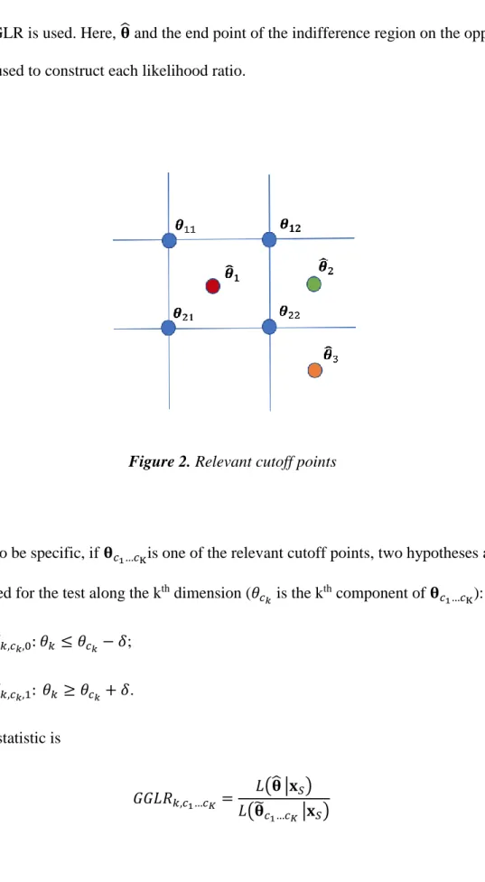
In grid multi-classification ACT, regardless of the actual number of cutoff points along each dimension, at most 2𝐾 (the number of endpoints a hypercube has) cutoff points around 𝛉̂ are relevant. Figure 2 shows an example with 𝐾 = 2 and 𝐶 = 3.

When 𝛉̂₁ is the ability estimate, all four cutoff points are relevant. However, when 𝛉̂₂ is the ability estimate, only two cutoff points 𝛉12 and 𝛉22 are relevant. Whereas when 𝛉̂3 is the ability estimate, only one cutoff point 𝛉22 is relevant. As 𝐾 tests are performed around each cutoff point, at most 2𝐾 _{× 𝐾}_{pairs of hypotheses around}_𝛉_̂_{need to be tested}

(52)

37 when GGLR is used. Here, 𝛉̂ and the end point of the indifference region on the opposite side are used to construct each likelihood ratio.

Figure 2. Relevant cutoff points

To be specific, if 𝛉_𝑐₁_…𝑐_Kis one of the relevant cutoff points, two hypotheses are formulated for the test along the kth dimension (𝜃𝑐𝑘 is the k

th_{component of}_𝛉

𝑐1…𝑐K):

𝐻_𝑘,𝑐_𝑘_,0:⁡𝜃_𝑘 ≤ 𝜃_𝑐_𝑘− 𝛿;

𝐻_𝑘,𝑐_𝑘_,1: ⁡𝜃_𝑘 ≥ 𝜃_𝑐_𝑘+ 𝛿. The test statistic is

𝐺𝐺𝐿𝑅_𝑘,𝑐₁_…𝑐_𝐾 = 𝐿(𝛉̂ |𝐱𝑆)

(53)

38 where 𝛉̃𝑐1…𝑐𝐾 = 𝛉𝑐1…𝑐𝐾 + 𝛅. The 𝑘

𝑡ℎ_{element of}_𝛅_is_{𝛿 × 𝑠𝑔𝑛(𝜃}

𝑐𝑘 − 𝜃̂𝑘) and all other

elements of 𝛅are 0. Here the sign function is defined as 𝑠𝑔𝑛(𝑥) = {

−1⁡𝑖𝑓⁡𝑥 < 0, 0⁡𝑖𝑓⁡𝑥 = 0, 1⁡𝑖𝑓⁡𝑥 > 0.

Figure 3 illustrates the end point of indifference region on the opposite side, 𝛉̃_𝑐₁_…𝑐_𝑘 when the test focus is on dimension 1. As 𝐺𝐺𝐿𝑅𝑘,𝑐1…𝑐𝐾 is always larger than 1, it is compared

to 1−𝛽

𝛼 to make classification decisions. The test stops only when all GGLR tests result in classification or ACT reaches the maximum test length. If the maximum test length is reached, classify the examinee based on the relative location of 𝛉̂ and the cutoff points. To take advantage of the correlation between dimensions and to facilitate classification, the maximum a posteriori (MAP) estimate is used as 𝛉̂.

(54)

39

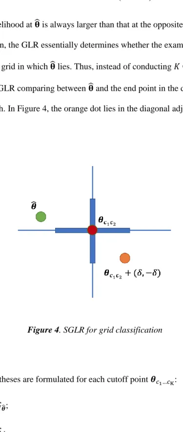
3.3.2 Simplified Grid Classification GLR (SGLR)

As the likelihood at 𝛉̂ is always larger than that at the opposite end point of the indifference region, the GLR essentially determines whether the examinee can be classified into the grid in which 𝛉̂ lies. Thus, instead of conducting 𝐾 GLR tests at each cutoff point, one GLR comparing between 𝛉̂ and the end point in the diagonally adjacent category is enough. In Figure 4, the orange dot lies in the diagonal adjacent category of

𝛉 ̂_.

Figure 4. SGLR for grid classification

Two hypotheses are formulated for each cutoff point 𝜽_𝑐₁_…𝑐_K:

𝐻𝑐0: 𝜽 ∈ 𝐺𝜽̂;