Mobility Modelling through Trajectory Decomposition and Prediction

(1)

Date of acceptance Grade

Instructor

Mobility Modelling through

Trajectory Decomposition and Prediction

Farbod Faghihi

Helsinki June 3, 2017

UNIVERSITY OF HELSINKI Department of Computer Science

(2)

Faculty of Science Department of Computer Science

Farbod Faghihi

Mobility Modelling throughTrajectory Decomposition and Prediction

Computer Science

June 3, 2017 71 pages + 0 appendices

Trajectory Prediction, Trajectory Analysis, Human Mobility, Mobility Modelling

The ubiquity of mobile devices with positioning sensors make it possible to derive user’s location at any time. However, constantly sensing the position in order to track the user’s movement is not feasible, either due to the unavailability of sensors, or computational and storage burdens. In this thesis, we present and evaluate a novel approach for efficiently tracking user’s movement trajectories using decomposition and prediction of trajectories. We facilitate tracking by taking advantage of regularity within the movement trajectories.

The evaluation of our approach is done using three large-scale spatio-temporal datasets, from three different cities: San Francisco, Porto, and Beijing. Two of these datasets contain only cab traces and one contains all modes of transportation. Therefore, our approach is solely dependent on the inherent regularity within the trajectories regardless of the city or transportation mode.

ACM Computing Classification System (CCS): A.1 [Introductory and Survey],

I.7.m [Document and text processing]

Tekijä — Författare — Author Työn nimi — Arbetets titel — Title

Oppiaine — Läroämne — Subject

Työn laji — Arbetets art — Level Aika — Datum — Month and year Sivumäärä — Sidoantal — Number of pages Tiivistelmä — Referat — Abstract

Avainsanat — Nyckelord — Keywords

Säilytyspaikka — Förvaringsställe — Where deposited Muita tietoja — övriga uppgifter — Additional information

(3)

ii

1 Introduction

Human mobility modelling is the study of people’s movement habits. It is used for the characterisation of movement patterns, for example, in transitions between different places or how the public transportation infrastructure is used. Understand-ing and characterisUnderstand-ing human mobility is a major scientific problem that has rele-vance to many scientific domains such as controlling epidemics [NW09, BGB11], analysis and forecasting of traffic [GLPC12, PZWS13, JWS08], urban planning [YZX12, ZLYX11, QLL+11], and numerous innovative mobile and network appli-cations [SBBK+_{11, ZLH13, HNT13, RZL}+_{12, SKJH06]}

An important usage of mobility modelling is in context aware computing. In or-der to provide a richer human-computer interaction, context can be utilised by the computers. Context aware computing was first introduced by [ST94] as a computer program that changes its behaviour adaptively according to its usage location and people and objects around it. From then, context aware mobile applications have grown at a great rate. In the beginning, it was a fundamental part of ubiquitous and pervasive computing applications, but over time it became an important part of desktop applications, web applications, mobile computing, and nowadays, a part of the Internet of Things (IoT) [PZCG14]. One of the key characteristics to derive context is location-aware computing by modelling user’s mobility [Gus02]. Mobil-ity models have been the focus of different studies, and they cover different key areas. Deriving important places in each user’s life by processing their movement traces [NB08], extracting the statistical characteristics of movement in terms of movement habit [SQBB10], and designing predictive models capable of predicting future movement behaviour of users [SMM+11] are a few of the examples in this area. These studies have predominantly focused on the movement between places; however, what is not known is how regular the movement between these locations are, i.e., how regular human movement trajectories are. In this thesis, our focus is on exploiting the existing regularity within movement trajectories which is mostly overlooked in the previous studies.

Existing research papers explore and analyse people’s movement data to detect and extract their patterns and characteristics [SQBB10, GHB08]. However, the results reported in these studies are based on very high levels of abstraction and low resolution data; one of the main reasons for this matter is the type of datasets used in the studies. The most common data source for these studies is call data records (CDR). CDR are the data that mobile operators receive and log based on

(6)

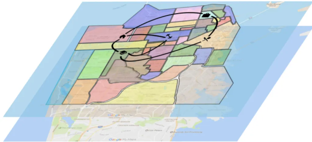
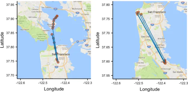
their users’ usage. For example, whenever users make phone calls, send messages, or change the cell-tower that they are connected to while moving the mobile operator will receive and log some data based on these actions. This data can be used to derive the user’s location by multi-lateration of radio signals between cell towers. The accuracy of the obtained location is heavily affected by the number of available cell towers and their positions. In best case scenarios, the approach can only derive the location in block levels; hence, CDR data constrains the accuracy at which we can analyse mobility, and it is not possible to study the movement behaviours in higher level of detail. Therefore, these studies mostly analyse the movement in terms of the transitions between different areas. Figure 1 displays an example of this kind of mobility analysis.

Figure 1: Precise analysis of movement trajectories is mostly overlooked by mobility modelling studies where their analysis is done in high levels of abstraction like the transition of the user in different areas of the city.

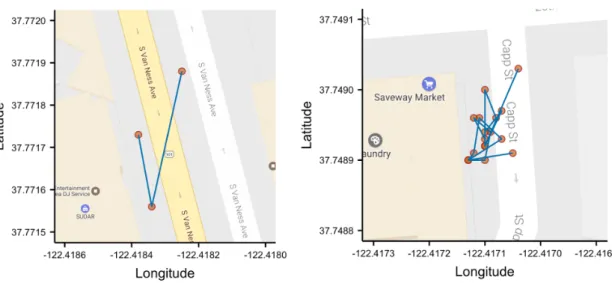
In addition, there are studies that take the movement data either with high accuracy like GPS traces or low accuracy like CDR location data as input and process them to extract the meaningful or distinct places for each user [LFK07, NB08, IBC+_12]. These places are those that have some meaning in user’s life like home, work place, gym, and favourite restaurant. After extracting these places, the movement between them is studied to create mobility models or analyse the predictability of transitions as illustrated in Figure 2.

In this work, we present a study on the regularity of route mobility. As mentioned, existing research has mostly overlooked the route mobility concept and does not

(7)

3

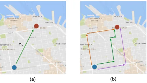
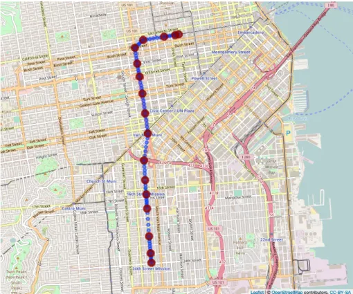
Figure 2: The movement data is processed first to extract the meaningful places for each person. The movement patterns between these places is studied afterwards. give any information regarding the actual path taken by the user for transitioning from one location to another, therefore the actual movement trajectory between locations is missing as illustrated in Figure 3 (a). By studying the route mobil-ity, we provide insights regarding the actual paths taken between any two points as shown in Figure 3 (b) and present how regular the movement between these points are. For this aim, we carry out our analysis using three different mobil-ity datasets in three different cities that contain different modes of transportation. Cabspotting [PSDG09a, PSDG09b] is the first dataset, which contains the GPS traces of more than 500 cabs from a one-month period in San Francisco. Ge-oLife [ZZXM09, ZLC+08, ZXM10] is the second dataset that contains the GPS traces of 182 users that has been collected over a period of five years, and most of the traces are in the city of Beijing. Finally, the last dataset is the Taxi Service Trajectories [MMGF+_{13, MMGF}+_{16], and it contains the GPS traces of more than}

400 cabs from a 24 day interval.

Everyday human mobility in urban areas is constrained by the urban infrastructure and road network; therefore, making the cabs of the two datasets a feasible proxy for human mobility. It’s worth mentioning that the datasets used in this work are freely available which assists in reproducibility of results. In contrast to the other studies that focus on the movement of each user or moving object, we analyse the movement trajectories in general which can be used for any user in the area of observations. As our first technical contribution, we develop a principled methodology for

(8)

mea-Figure 3: (a) The source and destination of a trip is known and can be used for studying the transition between places, but the information regarding the actual path taken between these two locations is missing. (b) Shows three different possible paths that a moving object can use to reach its destination.

suring the regularity of movement trajectories by computing the entropy of all tra-jectories for any given spatial and temporal resolution. For this aim, we convert the trajectories into Markov chains and quantify their regularity using Markov trajectory entropy [EC93]. Using this method, we analyse and quantify the overall regularity of trajectories and demonstrate that, as a whole, trajectories appear irregular and hard to predict. Consequently, we reveal that only a subset of points along the tra-jectories are responsible for irregularity within the trajectory. We extract and call these points fork-points. By representing the trajectories with their fork-points, we can show a higher predictability for them. Motivated by this result, as the second contribution of this thesis, we introduce a segmentation algorithm that segments the trajectories into more regular sub-segments. The segmentation can be used as an alternative compressed representation of the trajectories. Finally, we introduce a predictive framework capable of predicting moving objects trajectories.

(9)

5

2 Related Work

An extensive part of our work explores the human movement traces and analyses the inherent degree of regularity present within them. We categorise previous studies into three groups: human mobility, trajectory analysis, and energy efficiency. We first introduce the related work done in the area of human mobility which covers general characteristics of human movement. Next, we give an overview of trajectory analysis studies as our system relies on such techniques to provide predictions re-garding the destination and rest of the trajectory. Finally, due to the applicability of trajectory processing approaches in systems that provide energy efficient tracking, we mention the important works done in this area. In this section we provide a brief summary of the work done in the mentioned areas and discuss how our work differentiates from them.

2.1 Human Mobility

Human mobility patterns and the amount of regularity within them are studied in numerous scientific studies. These studies can be categorised either as mobility dis-placement modelling or characterisation of regularity within the movement patterns. Here we introduce the works done in each category.

In terms of the movement displacement, several key attributes have been discovered in different studies. It is shown that even though human motion is not a random walk, it can be modelled with Lévy flight [BHG06, GHB08, RSH+11]. According to the Lévy flight model, human movement consists of straight line trips with no pause or directional change which are known as flights. The length or distance of these flights follow a truncated power-law distribution – meaning that these travelling dis-tances decay as a power-law. In a similar way, it also means that these travels are mainly consisted of many small flights interleaved with longer flights. In another attempt [ZMH+15] Zhao et al. explains the shared features of human walks using Lévy walks by decomposing the movement patterns based on their transportation mode. Therefore, by having information regarding transportation mode, the Lévy flights can be broken into a mixture of log-normal distributions, while the flights in each mode contain power-law distributed jump sizes. Furthermore, other stud-ies [RSH+_{11, KKK06] have shown that in addition to the flights, the pause times} of human walks demonstrate a truncated power-law distribution as well. Another important characteristic of human motion as demonstrated in [GHB08] shows that

(10)

people will only move within a confined area; however, this confined area differs among people.

There are works that simulate individuals’ movement through human mobility mod-els [LHK+_{09, LHK}+_{12, MCN11, SKWB10]. These studies exploit human walking} traces and significant patterns in human mobility to create systems that are able to simulate human movement as realistically as possible. These systems exploit the identified features to simulate the human movement inside communities and areas such as university campus or companies. For pedestrian specific simulations, Blue et al. [BA01] uses Cellular automata microsimulation for simulating the pedestrians movement in discrete cells of 0.21m2. Yoon et al. [YNLK06] introduces a framework for statistical mobility model generation. To do this, they make use of coarse-grained wi-fi traces in a campus area.

Besides mobility displacement modelling, there have been studies investigating the regularity within human movement patterns, mainly the transitions between fre-quently visited locations. Song et al. [SQBB10] uses a dataset of call data records (CDR) to generate movement trajectories and investigate their predictability. The study reports an upper limit of 93% for predictability of human movement. How-ever, the user’s location in CDR data is a low resolution approximation; and hence, it contains a large amount of uncertainty. In a similar way, Lin et al. [LHL12] uses GPS data in order to have location data of higher resolution compared to call data records. The paper, used a grid model to provide a building level granularity and reported a 90% predictability for mobility. There are two main issues regarding these two papers. First, the mobility patterns are constructed with a fixed sampling rate. As a result, if a user visits multiple locations during this sampling interval, only one place will be represented for that time, which will lead in an incomplete reconstruction of user’s visitations. The other issue arises from the fact that the length of the location visitation sequence is determined by the sampling rate which affects entropy. Lu et al. [LWB+_{13] analyses movement patterns of individuals in} Cote d’Ivoire to measure regularity. Similarly, the authors reported an upper bound of 88%for predictability. In addition, Lu et al. shows that the mentioned limit can be reached by implementing Markov Chain based predictors.

While the previous studies analysed the data in high levels of abstraction, Smith et al. [SWGB14] explores the predictability of human movement by taking real-world topological constraints into account; therefore, reporting a more realistic and tighter upper bound. The study analyses the effect of sampling rate and spatial

(11)

7 resolution on the predictability and reports that the predictability upper bound is

11% to 24% lower than what previous studies have claimed. As a solution, Smith et al. suggests the integration of external data sources to improve the predictions based on the application requirements. De Domenico et al. [DDLM13] reveals a relationship between social interactions and mobility. The study combines the data regarding user’s social interactions with movement data and improves the accuracy of user’s position predictions.

Li et al. [LJH+14] analyse movement predictability in terms of vehicular mobility. For this aim, they focus on predicting the next most likely major intersection along a route. For deriving a predictability limit, entropy theory is used. The research reports the predictability of vehicular mobility to be larger than 78%; therefore, showing presence of a strong regularity in the movement patterns.

This thesis provides the first ever study of regularity of route mobility. We demon-strate that movement trajectories can be decomposed into sub-segments with high predictability, despite using a very small set of points along the route for predicting the route accurately. Compared to the previous studies, we use trajectories in high level of details.

2.2 Trajectory Analysis

A trajectory captures a moving object’s path through space as a function of time. Hence, a trajectory represents the path taken by a moving object and is an im-portant piece for modelling and analysing its movement. Even when trajectory information is missing, studies make assumptions regarding trajectories or try to approximate them. For example, Zheng et al. [ZHL06] studies the effect of social activities on users’ whereabouts. They combine social attributes with geographical data to derive their location based on a survey data. Since the survey data contains no trajectory information, Dijkstra’s shortest path algorithm was used for recreating the paths. But not all studies use the information regarding the actual trajectories. These studies mostly use the trajectory data only as an input data to derive other information such as places that each user visits. In [LZX+_{08], Li et al. uses the GPS} traces of 65 users over 6 months in order to provide a similarity measure to match more alike users with each other based on their movement behaviour. They intro-duce a framework named hierarchical-graph-based similarity measurement (HGSM) that is based on user’s location visitation history. Therefore, the GPS trajectories are only used to detect user’s distinct location visitations.

(12)

One of the first works to focus on trajectory tracking was proposed by Lange et al. [LFDR09]. The study tracks and processes the actual trajectory of a moving object and simplifies it according to a certain accuracy bound to provide an ap-proximation. Liao et al. [LPFK07] uses GPS traces to capture regularity within user’s movement behaviour. Accordingly, their model is able to detect undefined or irregular behaviour within mobility patterns of a user. Their system is built upon a hierarchical Markov model that uses Rao-Blackwellized particle filters at different hierarchical levels to provide a more efficient inference for user’s destination and mode of transportation. Our model can capture the regularity of all user’s in an geographical area and we are able to show why some movement might be irregular. In a series of studies, Krumm et al. analyse GPS traces to create predictive mobility models. In [Kru06, KH06] destination prediction based on a probabilistic approach is presented with the intuition that drivers choose efficient routes. In a similar ap-proach they use a grid representation of the world for discretisation of trajectories. What differentiates our work from these studies is that we analyse the human move-ment trajectories in a more general level. We make no claim regarding the users’ mode of transportation as we aggregate all movement trajectories of all users to-gether. In addition, our model is able to predict the path in addition to destinations. In [Kru10] the author uses a dataset of driver’s turning decisions at intersections to predict the driver’s route. This approach can be used to predict the trajectory, but it can only provide prediction at the intersection for the next segment of the trip and not the whole trajectory.

2.3 Energy Efficiency

Tracking user’s movement and extracting his position in a continuous matter and with high accuracy using mobile sensors such as GPS sensor can be costly action in terms of energy. Therefore, providing energy-efficient tracking for mobile devices requires exploring and analysing of movement of users and their corresponding tra-jectories. For this reason, we have decided to introduce a selection of these studies that are related to mobility in this section.

Most of the first works on energy-efficient mobility monitoring focused on opti-mising energy consumption by reducing the sampling rate of GPS receivers. We can categorise these into two groups. The first group depends on the fact that the accuracy requirement of localisation varies. Moreover the reduction of sam-pling is done by either using less expensive alternative localisation methods such

(13)

9 as Wi-Fi and cell-tower triangulation – whenever it is allowed by the accuracy re-quirements [LKLZ10, PKG10] – or by exploiting other external information that can provide information regarding the movement. SensTrack [ZLJG13] system uses the information regarding the acceleration and direction derived from the less expensive sensors to trigger GPS sampling. Whenever a user moves indoors, he uses WiFi localisation. The study is related to our work where it uses a Gaussian process regression method to reconstruct the trajectories from partial samples. The stored samples are similar to the fork-points that we use to decompose the trajectory, but unlike our work they are not related to the regularity of movement. Fang et al. [FZ11] exploits the information regarding constraints and limitations on daily movement. The authors present EnAcq, a trajectory data acquisition scheme that utilises the information regarding the road networks with map matching techniques to improve energy consumption. In order to reduce energy usage, Nodari et al. [NNS15] model movement trajectories. The approach samples and communicates the location only when the moving object deviates from predicted trajectory.

The other group of studies that are relevant to our work, utilise line simplification methods, such as Douglas Peucker [DP73], to simplify the actual trajectory with an approximation. The points in the compressed trajectory do have similarities to our detected fork-points that can be used to compress the trajectories as well. Lange et al. [LDR11] use line simplification techniques to reduce the sampling rate and at the same time use dead reckoning to select communication intervals. Constandache et al. [CGS+_{09] introduce EnLoc, an energy efficient localisation framework. EnLoc} exploits the regularity of users’ movement. By using the habitual characteristic of mobility, it predicts the population’s location to provide an offline optimal solution for energy efficient localisation. The EnLoc system schedules location updates at so-called uncertainty points, which roughly correspond to fork-points in the context of our work. Entracked [KBBN11, BBKN15] is another system for trajectory tracking. In EnTracked, application designers provide a desired degree of accuracy for position and/or trajectory tracking accuracy and the system determines the optimal strategy to achieve the desired accuracy with the least amount of energy. The system design of EnTracked combines intelligent sensor management strategies with trajectory simplification techniques and intelligent uploading policies to preserve energy. It is worth mentioning that there are also other approaches that provide optimal approaches without the reduction of sampling. For example, instead of adapting GPS duty cycle, Ramos et al. [RZL+11] propose the LEAP system which saves energy by offloading computationally intensive parts of the GPS processing pipeline

(14)

to a server or cloud platform. We exclude detailed discussion about these works as they do not take advantage of human mobility analysis for energy reduction.

(15)

11

3 Data Collection

We analyse regularity in route mobility using three different datasets that contain the movement trajectories of moving objects. Spatial trajectories contain rich infor-mation that can be utilised in different applicable areas, but because of the way they are captured and stored they contain may contain noise and inaccuracies. Therefore, they should be first processed according to our needs.

We have performed our analysis using three different datasets. Cabspotting [PSDG09a, PSDG09b], which contains GPS traces of more than500 cabs from a one-month pe-riod in San Francisco; GeoLife [ZZXM09, ZLC+_{08, ZXM10] contains the GPS traces} of 182 users that has been collected over a period of five years, and most of the traces are in the city of Beijing; and finally, Taxi Service Trajectories [MMGF+_13, MMGF+16], which contains the GPS traces of more than 400 cabs from a 24 day interval.

In this chapter we cover the concepts that enable us to process our spatial data and making it ready for our computations. We first summarise the factors that are intertwined with collecting spatial data. Next, as in our case the data is already collected, the majority of this section describes the techniques required for processing the spatial trajectories to be transformed to a clean and ready-shape version for our analysis. Finally, we close this chapter by demonstrating the datasets after the post-processing steps.

3.1 Trajectory Preprocessing

To record the continuous movement of an object we need to sample it in the form of discrete points. This will lead into storing an approximation of the continuous movement. The higher the sampling rate, The higher the accuracy of the original movement in the samples.

Even though more accurate representation of the movement is desired while working with trajectories, there are certain factors that prevent us from collecting the most accurate trajectories. For example, the higher the sampling rate the larger the number of measurements will be, which can lead into massive datasets. In addition, higher sampling rates also require more network communication to transmit the samples. Therefore, storage space and network communication capacity are two of these constraints. To overcome this issue, simplification methods are proposed to

(16)

save storage and communication costs and remove redundant data.

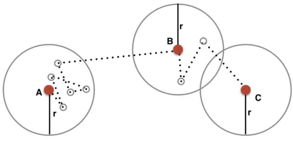
Figure 4: Point policy is an update policy where an application specific error distance (r) is selected. From each sampled location, a new sample is only recorded when the object moves further than the error threshold from its previous sampled location. Gathering more samples puts a computational burden on the devices leading into higher consumption of energy. Reading continuously from energy expensive track-ing sensors like GPS can deplete energy much faster. To address this issue, the research community has proposed several solutions. These studies integrate meth-ods such as dead reckoning to estimate the future position of the object based on its previously known location, direction, speed, and time. This information can be extracted from available tracking sensors such as accelerometers and gyroscopes. By using this approach it is possible to reduce the usage of energy hungry sensors like GPS. In addition, update schemes are used to decide when to store or communicate the location of a device. Point policy [CJNP04] is an example of a simple update policy. As illustrated in Figure 4, point policy defines an error threshold and only stores or reports the position when the user moves beyond the defined error thresh-old. Therefore, an application specific error threshold can be selected for the point policy to store a sample of the movement. There are advanced methods such as the Douglas-Peucker algorithm [DP73] that can be used for approximating the original trajectory. More advanced works in the area of energy efficient tracking have already been discussed in Section 2.

(17)

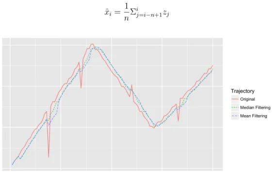
13 An important factor is the inherent error present in the tracking devices. For ex-ample, when using call data records (CDR) to track the user, the derived locations contain a high amount of error. Thus, it is not meaningful to capture the location for every few seconds. GPS sensors, on the other hand, have an average error of 10 meters. At times during the sampling of movement, the observed position may have much higher error which is not in line with other samples leading to the cre-ation of outliers in the captured data. Due to the captured noise, the trajectories are never perfectly accurate. To solve this issue, it is possible to use a variety of filtering techniques. In order to familiarise the reader with this issue we provide an example trajectory and describe two simple filtering methods to resolve the noise. The first simple method to remove the noise is to use a mean filter. Mean filtering works as sliding window that covers the lastntemporally adjacent values of the last observation z. Therefore, calculating the mean of the lastn observations. Equation 1 describes the mean filtering.

ˆ xi = 1 nΣ i j=i−n+1zj (1)

Figure 5: The captured noise in trajectories can be removed by using the filtering methods. Both median and mean filtering introduce lag to the original trajectory; however, unlike mean filtering, median filtering is not sensitive to outliers.

Two downsides of the mean filtering is that it introduces some lag to the original trajectory, and its sensitivity to outliers. Figure 5 displays a trajectory before and after mean filtering with a window of size five is applied to it.

(18)

The second method that we describe here is called median filtering and it can be used to mitigate the mean filters sensitivity to the outliers. Median filtering, as described in Equation 2, is similar to the mean filtering. The only difference is that we take the median of the last n observation instead of the mean:

ˆ

xi =median{zi−n+1, zi−n+2, ..., zi−1, zi} (2)

Both techniques have the disadvantage of adding lag to the original trajectory. The aim of introducing filtering in this section is to only help the reader to under-stand the characteristics of real world data better. For more advanced filtering techniques, we invite the readers to look into Kalman filtering [Gel74] and Particle filtering [DDFG01].

3.2 Cleaning Datasets: Postprocessing

In every data collection there are different factors that can affect the quality of the captured data. These factors can be related to the accuracy of the sensors or the approaches used for the study. Based on available resources and tracking devices, their energy capacities, and their average error level, a meaningful sampling rate is chosen. Thus, there is a trade-off between the accuracy of the captured trajectory and the available resources. In addition, different applications may need data with certain standards which may be different than the original application that led into the data collection study.

In our work we use three different datasets for our experiments, and we have to process and clean these datasets to meet our desirable level of quality. In this section, we discuss the methods needed to process and format the datasets according to our needs. We first discuss the general principles for cleaning the datasets and provide specific thresholds values used by cleaning methods for each dataset in Section 3.2.4. This will enable our readers to follow the steps we took to produce the results.

3.2.1 Velocity pruning

In analysing the regularity of route mobility, it is important for the data to have sufficient degree of accuracy so that it would provide a good approximation of how people move. One attribute that we can use to see if the trajectory is faulty is to check the velocity between any two consecutive observations. After computing the

(19)

15

Figure 6: Two sampled trajectories from the Cabspotting dataset is shown. It is evident that both of the trajectories have unrealistic segments that look like very long jumps which are faulty. The trajectories that contain segments with unrealistic speed values are removed.

velocity, we remove any trajectory that contains a pair of observations with unreal-istic speed. The removal of segments where speed is not within the possible velocity range of that metropolitan area is called velocity pruning. Therefore, all trajec-tories that contain a segment with an unacceptable speed value are removed from the dataset. Figure 6 illustrates two examples to provide a better understanding regarding how the velocities above the maximum range may affect the trajectories.

3.2.2 Trip Merging and Pruning

Another characteristic that can be used to remove faulty trajectories is the distance between the source and destination of a trip. There are trips where the distance is really small for the trip to be meaningful, which can correspond to either erroneous observations or cases where the user did not start any trips but was recording some observations. Figure 7 provides two examples of such trips. We remove any trip that has an overall distance smaller than a threshold.

(20)

Figure 7: Two sampled trajectories from the Cabspotting dataset is shown. The distance between the source and destination of some trips is too small to be a representation of an actual trip. These cases are removed from the dataset.

information regarding the trip. For example, a trip that lasted for 10 seconds is not meaningful to be counted as a real trip. Any duration for trips that are not within a selected range is removed.

3.2.3 Distance and Update Rate Between Consecutive Samples

As already mentioned, each spatial trajectory in the dataset is made of discrete data-points. Therefore, there is a gap between any two consecutive data-points. Based on the size of these gaps there are three different cases. First, if the size of the gaps is small the quality of the trajectory is at a desirable level; thus, nothing needs to be done. Second, the length of the gaps in some cases are bigger than what is required for our application but still reasonable. In such cases we can reduce the length of these gaps, and reconstruct the original path using linear interpolation, which is discussed later. Finally, in some cases the gap between two consecutive observations is too large to be meaningfully filled by linear interpolation. Figure 8 illustrates two instances of such cases. Trips that contain these non-useful segments are removed as part of the cleaning pipeline.

(21)

be-17

Figure 8: Two sampled trajectories from the Cabspotting dataset. In some cases, the gaps between any two consecutive observations of a trajectory is too big to be meaningfully filled with linear interpolation.

tween every consecutive observation can affect the linear interpolation. Thus, all trajectories that contain a segment of consecutive samples where the update inter-val is bigger than a threshold are removed.

3.2.4 Dataset Specific Thresholds

Each of the three selected datasets for our study has their specific level of quality. Accordingly, we have selected a set of thresholds to have the best possible level of accuracy in each dataset. All threshold values are stated table 1.

Since Cabspotting dataset contains traces both when cabs had a passenger and when they were empty, we remove all the empty cab traces in addition to the described

(22)

Table 1: Threshold values used for cleaning for each dataset

Cabspotting Geolife Taxi Service Trajectories

Velocity Threshold 34m/s 34m/s 34m/s

Minimum Trip Distance 250m 200m 250m

Minimum Trip Duration 60s 30s 60s

Maximum Trip Duration 14400s 14400s 14400s

Maximum Sampling Inter-val

180s 180s 180s

Maximum Consecutive Samples Distance

1000m 400m 300

cleaning steps for all the datasets.

3.2.5 Interpolation

Because of the update interval between two position readings, we might still have gaps in the extracted trajectories. To get rid of the gaps, we use linear interpolation on the sequence of cells as an approximation for missing cells in the trajectory. To clarify, assume we have two data points P1 and P2 with the following coordinates,

(x1, y1) and (x2, y2). If we want to fill in the gap between these two points, we consider each axis separately. Here, we explain how the linear interpolation works on one axis, and the value on the y-axis can be calculated in a similar way. Let P1 andP2 be sensed at timest1 andt2 respectively. Therefore, in order to approximate the valuext on x-axis at some timet between t1 and t2, we calculate:

xt=x2−(x2−x1)

(t−t1)

(t2 −t1)

(3) We use interpolation to reduce the time interval between the data points to ten seconds. We did not choose a smaller value for the interval between the updates since we might introduce harsh oscillations to our trajectories. After this step, we remove those traces that still contain gaps. We have categorised trip trajectories into different groups based on their source. Each of these trajectories Ts,d consist

of a sequence of n cells c1, ..., cn, where c1 = s and cn = d. Whenever the moving

(23)

19

Figure 9: Interpolation example

of the trajectories in our system that have the same cell as their source for the next step of processing. Before going further, we have to demonstrate the necessary tools for measuring regularity.

3.3 Grid Transformation

To analyse and quantify the regularity of trajectories, we use a grid network model over the world. We then discretise the trajectory data by mapping each observation into a discrete grid cell. The mapping is done by converting each longitude and latitude pair into a cell index on ad×dsized grid according the algorithm described by Nurmi et al. [NBK10]. Figure 10 illustrates an example of using a grid network to discretise a trajectory into multiple cells. This enables us to be able to index the data points to grid cells and aggregate all the corresponding data points in one cell together. Accordingly, each mobility trace will become a sequence of grid cells. Using a grid model to discretise the trajectories has some advantages. Discretising

(24)

Figure 10: Before being able to use our data for regularity analysis, we discretise the trajectory using a grid model into discretised cells.

the measurements is essential for computational tractability, and helps to overcome inaccuracies in location measurements, e.g., due to driving on a different lane or due to inaccurate GPS fixes.

In our analysis, we use different cell sizes for each of the three datasets based on their average sampling rate. Cell sizes: 400m×400m, 200m×200m, and 250m×250m

are selected for the Cabspotting, Geolife, and Taxi Service Trajectories datasets, respectively. The cell sizes are selected as a trade-off between location accuracy and computational requirements. Choosing lower values ford results in trajectories with higher resolution, but such values will lead to inaccurate trajectories since the original dataset’s observations did not have the required accuracy.

As a final step, we have to make sure that the source is always connected to the destination. It means that from any cell, the next cell along the path should be one of the eight neighbours of the current cell. Therefore, after the discretisation of the trajectories, we again remove any trajectory that may end up with a gap.

3.4 Data Description

Before moving into the regularity analysis chapter, it is worth looking into some statistics describing the final cleaned datasets to get more familiar with them. After the cleaning pipeline, Cabspotting dataset has 535 unique users and 318,011

(25)

21 distinct trajectories, Geolife dataset has 173 unique users and 41,756 distinct tra-jectories, and Taxi Service Trajectories dataset has 439 unique users and 945,881

distinct trajectories. Table 2 provides more detailed statistics for each dataset after the cleaning process.

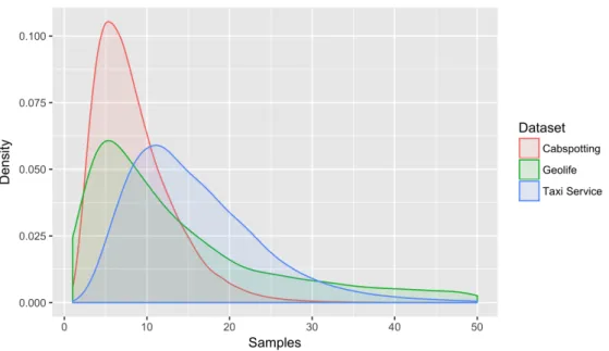
After discretising the data using a grid network, each trajectory is then defined by a sequence of cells. Figure 11 shows the distribution of lengths of the trajectories. We can observe that the trajectories in the Cabspotting dataset have less variety compared to the other two datasets, and the average length of its trajectories is just a bit over five cells. Thus, this dataset has mostly short trajectories. This is mainly because of the larger cell sizes used for discretisation in the Cabspotting dataset because of its relatively poor quality compared to the other datasets. In addition, compared to the other datasets, Cabspotting contained more errors; therefore, more trajectories got removed during the cleaning process.

Figure 11: The distribution of discretised trajectory length for each dataset.

On the other hand, Geolife trajectories contain more variety but still the mean of the trajectory lengths is around five samples, just like the Cabspotting dataset. Considering the fact that we used the smallest cell size for the Geolife dataset, it might be expected that the dataset should have longer trajectories, but it should be taken into account that in addition to the driving trajectories, Geolife dataset contains other modes of transportation like walking. This is one of the reasons that

(26)

Table 2: Cabspotting dataset after cleaning Cabspotting Maximum consecu-tive points distance Maximum sampling rate Maximum trip dura-tion Maximum trip dis-tance Maximum segment velocity Minimum 140.306 21.000 60.000 250.074 0.145 1st Quartile 473.201 109.000 301.000 1207.944 7.047 Median 545.905 129.000 450.000 1894.011 9.312 Mean 553.619 147.667 501.730 2189.747 9.533 3rd Quartile 630.594 175.000 640.000 2853.580 11.833 Maximum 1101.062 6713.000 9880.000 11456.437 33.988 Geolife Maximum consecu-tive points distance Maximum sampling rate Maximum trip dura-tion Maximum trip dis-tance Maximum segment velocity Minimum 55.567 5.000 30.000 200.071 0.163 1st Quartile 214.729 98.000 325.000 503.792 4.064 Median 247.327 172.000 697.000 1204.249 11.288 Mean 254.859 228.467 1003.558 3278.627 12.031 3rd Quartile 287.981 270.000 1293.000 3584.881 18.815 Maximum 520.612 12009.000 14021.000 101859.025 33.998 Taxi Service Trajectories Maximum consecu-tive points distance Maximum sampling rate Maximum trip dura-tion Maximum trip dis-tance Maximum segment velocity Minimum 99.951 15.000 60.000 250.049 0.050 1st Quartile 327.045 90.000 375.000 1306.066 11.395 Median 363.153 105.000 540.000 2015.175 13.985 Mean 363.443 143.198 629.459 2299.213 13.678 3rd Quartile 399.784 150.000 765.000 3028.302 16.499 Maximum 679.239 13455.000 14295.000 47779.620 20.000

(27)

23 originally Geolife trajectories are shorter compared to the other two datasets. For the Taxi Service Trajectories we have more variance compared to the other datasets and also longer trajectories in general. In the Taxi Service Trajectories dataset the mean of the trajectory lengths is around11cells. While the dataset is similar to the Cabspotting dataset in terms of transportation mode, relatively it has higher quality trajectories. We also selected a cell size smaller than the one used for discretising the Cabspotting. Therefore, generally longer trajectories were expected for the Taxi Service Trajectories dataset.

(28)

4 Trajectory Regularity

Previous studies on human mobility have demonstrated that individual mobility patterns, characterised by transitions between important locations, are predictive to a high degree [LWB+_{13]. While the regularity of location transitions has been} established, less is known about the routes that people take while transitioning between locations. That is to say, the regularity of human movement trajectories has mostly been overlooked and no conclusive information is available.

Individuals’ everyday movements are affected by different factors, which make them more regular. As an example, consider the movement trajectories of a person that has several frequently visited locations, such as home and work. His movement trajectories between these locations tend to overlap to a high degree since the person usually takes the same familiar path. In addition to the personal attributes of a person, the movement trajectories are also constrained by the overall structure of road networks and public transportation routes.

In this section we describe methods for quantifying the amount of randomness present in movement trajectories. We first demonstrate how to use the discretised trajectory data, so that we can use the Markov chains. Next, entropy is described and used to quantify the irregularity of each discrete cell. Then the entropy of the Markov trajectories is presented as a way to quantify the randomness between any source and destination. Finally, the entropy of conditional Markov trajectories is discussed as means to measure the irregularity of trajectories by conditioning on an intermediate cell.

(29)

25

4.1 Representing the Trajectories as Markov Chains

In the previous section, we have shown how to discretise GPS traces into a 2-D coordinate systems with square-shaped cells. As an example consider Figure 12, which shows a movement trajectory discretised over square cells. Here, the tra-jectory takes on a path passing through the cells C4,1, C4,2, C4,3, C3,3, C2,3, C1,3, C1,4.

Therefore, each trajectory is a sequence of transitions between subsequent cells start-ing from the source cell and endstart-ing at the destination cell. We quantify regularity of trajectories by modelling them as (first order) Markov chains. Each cell along a trajectory corresponds to a state in a Markov chain and movements from one cell to another correspond to transitions between states. We construct a transition matrix based on the trajectories and compute the corresponding probability tran-sition matrix. Given the collection of all trajectories T, we create a Markov chain

M(T) by constructing a transition probability matrix P = pi,j where pi,j denotes

the probability of observing a transition between grid cells i and j. Next, as an initial attempt to analyse the regularity, we calculate the entropy of each state to learn about their irregularity. Entropy described by Equation 4 is a measure from Information Theory, and it is used to quantify the unpredictability of a state.

H(X) = Σn_i₌₁P(xi)I(xi) = −Σni=1P(xi)logbP(xi) (4)

In general, it is possible to have a transition between any two states of the Markov chain. Since we are using a grid model and the generated Markov chain is a repre-sentation of our trajectories, the only transition is possible from any state is only to its eight neighbours as illustrated in Figure 13. Therefore, P(xi) from Equation 4

corresponds to the probability of the transition between the current cell and its i’th neighbour. Based on this constraint we can re-write Equation 4 as follows:

H(X) =−Σ8_i₌₁P(xi) log2P(xi) (5)

In the case where the transition probability is evenly distributed between all the neighbours – meaning that the current state contains the highest amount of irregu-larity – Equation 5 is equal to the value3. On the other hand, if all the transitions from the current cell are to one of the eight neighbours – meaning that the outcome of the transition from this cell is completely predictable – the Equation 5 will be equal to 0. As a result we can see that the cell entropy value is bounded as follows:

(30)

Figure 13: In our application environment, the only possible transitions from any states is to its eight neighbours.

0≤H(X)≤3 (6)

We modelled the trajectories of the three datasets as (first order) Markov chains. Next, we calculated the popularity of each cell by counting the number of times the cell was visited by different trajectories. Furthermore, we computed the entropy for all states. Finally, we have plotted the results using heat-maps as illustrated in Figure 14.

Consider Figure 14, in cell visitation figures (a, c, e) we can locate the areas where most of the movement trajectories are concentrated. Since we have the smallest cell size and highest sampling resolution for the Geolife dataset, we can observe that the dense areas are mostly around the main roads. Because of the higher cell sizes for the other two datasets, there is no specific paths where the trajectories would be concentrated around. Nevertheless, based on the cell irregularity plots (b, d, f) of all three datasets, it is obvious that there are only a subset of cells in the dense areas where they demonstrate the highest amounts of irregularity. This is in line with our assumption that trajectories consist of more regular segments connected by highly irregular points that are responsible for most of the irregularity exhibited by the trajectory. In the next section, we look into the cell entropies along the path in more detail.

(31)

27

Figure 14: a, c, and e display the popularity of each cell by computing theloglog(x)

where x is the number of visitations to that cell. b, d, and f shows the amount of irregularity within each cell by computing 2x _{where x is the cell entropy.}

(32)

Figure 15: For Cabspotting and Taxi Service Trajectory trajectories, the most pop-ular source is selected. Accordingly, based on the trajectories that start from the selected cell, five popular destinations are selected.

4.2 Distribution of Entropy within a Trajectory

To gain more familiarity with cell entropies within a trajectory, we select the most popular source cell (cell where highest number of trajectories started from) of the Cabspotting and Taxi Service Trajectories datasets. For Cabspotting dataset,

11,888trajectories start from the most popular source cell. For Taxi Service Trajec-tories, this number is 38,024. Next, we select five of the most popular destinations based on the trajectories starting from the previously chosen source cell. Figure 15 shows these cells for the two mentioned datasets.

As the next step, we randomly sample one trajectory from each of the selected source destination pair which gives us five trajectories for each dataset. We match all the cell entropies along the trajectories and interpolate them along 20 points, so that they are of the same length. Figure 16 shows the interpolated cell entropies for the five selected trajectories of each dataset. Since a large number of trajectories start from the selected sources, we can observe that the cell entropy is relatively high at the beginning of the trip. As we progress along the paths, there are points where the entropy becomes relatively low that results in higher predictability of the next transition.

Cells with high local entropy value appear as peaks in our plot. These correspond to decision points where trajectories start to deviate from each other, these are namely

(33)

29

Figure 16: Cell local entropies along five different trajectories chosen from the two datasets between the most popular source and five popular destinations.

our fork-points. Having knowledge about the transition from the fork-point for a moving object gives higher information for predicting the future of the trajectory. The segments created by these fork-points are highly regular; therefore, it is our desire to extract the points that are mainly responsible for the amount of randomness in a trajectory to be able to encode the whole trajectory with them. The fork-points in each trajectory can help us to split the trajectories into segments that have higher regularity. In Section five we introduce an algorithm for segmenting the trajectories into these more regular segments by using fork-points. In the next section, we look into the quantification of randomness within trajectories as a whole.

(34)

4.3 The Entropy of Markov Trajectories

We are interested in a method that enables us to quantify the overall amount of ran-domness within a trajectory. We use the entropy of Markov trajectories as described by Ekroot et al. [EC93] to quantify the randomness of trajectories in a irreducible finite state Markov chain. To model the discretised trajectories of all datasets, we created a transition matrix. The size of this square matrix depends on the total number of cells after discretisation. Therefore, if we haven unique cells in our grid network, we create a transition matrixTn,n. We compute the frequency of each

pos-sible transition in the dataset and update the transition matrix accordingly. Next, we extract the probability transition matrix Pn,n as an intermediate step in order

to be able to compute the Markov trajectory entropies. Pn,n can simply be created

fromTn,nby summing the values in each row, and dividing the values of each row by

the calculated sum. The value ofPi,j corresponds to the transition probability from

state i to state j. Using the constructed Markov chain, it is possible to represent the trajectories of a moving object as a weighted random walk on a graph. In such a graph, each trajectory cell is represented by vertices and possible transitions by edges. This graph is known as the state transition diagram.

In order to compute the entropy of Markov trajectories, we create a trajectory entropy matrix H, and we use an example along the steps for better understanding. Figure 17 displays the state transition diagram of a 5-state Markov Chain with the probability transition matrix of:

P5,5 =         0 0.7 0.3 0 0 0 0 0 0 1 0 0.2 0 0.8 0 0 0 0 0 1 0.6 0 0 0.4 0        

The associated state entropy rate of the given Markov chain example is given by:

H(χ) =−Σi,jµiPi,jlogPi,j (7)

In Equation 7, µ is the stationary distribution and can be calculated by solving

µ=µP. A trajectory T from the source i to the destination j is presented as Ti,j,

in which no intervening state is equal to j, and we want to compute the trajectory entropies H(Ti,j). A general closed form solution used for computing the H(Ti,j) is

(35)

31

Figure 17: State transition diagram for a 5-state Markov Chain.

as follows:

H =K−K˜ +H∆ (8)

The matrix H∆ is the entropy rate of a state. It is a diagonal matrix with entries

(H∆)i,i = H_µ(χ)

i· . Here H(χ)is the entropy rate of a state. Equation 9 describes how

to calculateH∆.

H(χ) =−Σi,jµiPi,jlogPi,j (9)

And matrix K in Equation 8 can be calculated using:

(I−P +A)−1(H∗−H∆) (10)

˜

K is a matrix in which the element onith row and injth column equals the diagonal elementKj,j ofK; A is the matrix of stationary probabilities with entriesAi,j =µj;

H∗ is the matrix of single-step entropies with entriesH_i,j∗ =H(Pi·) = −ΣkPi,klogPi,k;

and H∆ is a diagonal matrix with entries(H∆)i,i = H_µ(χ)

i·

Now, we are able to compute the matrix of trajectory entropies Hn, nas described by Equation 8. Hn, n contains the entropies of the trajectories between any two

(36)

cells in the extracted data points. For our example Markov Chain we would get the following Markov Trajectory entropies:

H5,5 =         2.7161 1.9555 6.7135 3.3746 1.0978 1.6182 3.5738 8.3318 2.9957 0 2.3401 3.5810 9.0537 1.3210 0.72192 1.6182 3.5738 8.3318 2.9957 0 1.6182 3.5738 8.3318 2.9957 1.6296        

For example, the entropy of the T1,5 trajectory is 1.6296 bits, while the entropy of deterministic trajectories – meaning the transitions are completely predictable –

T4,5 and T2,5 is equal to zero which means that these trajectories do not contain any randomness.

Previously, we gave an example of how people move between important places. For example, people tend to commute on the same path between their home and work. We made an assumption that for these more frequent routes, there will be more regularity present. To investigate this matter, we have extracted all the trajectories starting from the most popular source in each dataset and computed the Markov trajectory entropy matrix. We can observe from the result, as shown in Figure 18 that our assumption was in fact true. The more trips we have for a given source and destination, the more regular the paths are. In the next section, we look into how knowing which cells are visited between a source and destination changes the entropy of Markov trajectories. Up until now, we analysed the trajectories by discretising them into states and showing that some of these states have much lower uncertainty than others. Then, we described the entropy of Markov trajectory which enables us to compute the randomness within any complete trajectory between any two locations. Next, we introduce entropy of conditional Markov trajectories which helps us to compute the trajectory entropy after conditioning on an intermediate cell.

4.4 The Entropy of Conditional Markov Trajectories

Based on the technique introduced by Ekroot and Cover [EC93], we were able to calculate the amount of randomness in an irreducible finite state Markov chain. Therefore, we were able to compute the entropy of the trajectory between any two states in the graph that models the user’s mobility. However, if we gain new

(37)

infor-33

Figure 18: The Markov trajectory entropy is computed for all the trajectories started from the most popular source for all three datasets. There is a decreasing trend in the trajectory entropy values as we observe more trajectories between a source and destination.

mation that the user passed through states on its path to reach the destination, we cannot utilise the new information with the previous approach. Here, we describe a method for computing the entropy of conditional Markov trajectories by introducing a way to transform the original Markov chain so that it expresses the conditional distribution of trajectories based on the work done by Kafsi et al. [KGT13].

To understand this matter better, consider the following example. Based on our ex-ample Markov Chain shown in Figure 17, we computed the entropy of the trajectory between the two states 1 and 5 to be 1.6296 bits. If we learn that the user has gone through state number 4 before reaching the destination, we would like to compute the trajectory entropy T1,5 conditioned on visiting the fourth state along the way.

(38)

Before going further and describing the entropy of conditional Markov trajectories, it should be noted that the additive property does not hold for the entropy of Markov trajectories. Based on our example we would have theH1,4+H4,5 = 3.3746but after conditioning on visiting the fourth state and computing the conditional entropy we getH1,5|4 = 0. Therefore, it is evident that the additional information about the user passing state number 4 makes the trajectory fully predictable. By extracting such intermediate states, it is possible to fully encode the trajectory. Therefore, if there exists a set of intermediate cells such that by conditioning on them the conditional entropy of Markov trajectories becomes zero – meaning the path changing into being fully predictable – we can break the whole trajectory into segments connected by the cells of this set. As a result we would have fully regular segments, connected by the decision points.

Before going through the algorithm for computing the entropy of conditional Markov trajectories, we first demonstrate a few concepts that are needed for the algorithm. We can define the conditional entropy of a trajectory between the source s and destination d, Ts,d, that passes an intermediate state u by:

Hsd|u =H(Tsd|Tsd ∈ Tsdu)

=−Σtsd∈Tsdup(tsd|Tsd ∈ T

u

sd)logp(tsd|Tsd ∈ Tsdu)

where Tu

s,d is a set that contains all the trajectories between the source s and the

destination d that go through the intermediate state u. Now consider a sequence of intermediate cells u =u1u2...ui. Then Tsdu is the set of all trajectories in the set

Tsd that visits every intermediate cell inu in order, before reaching the destination.

The entropy of the trajectory between sources and destination dwhere it visits the intermediate cells u is:

H(Tsd|Tsd ∈ Tsdu) = l−1 X k=0 H_u kuk+1|d¯+Huld (11) where u0 is the source s.

As part of the algorithm we have to compute the entropy of the Markov trajectories which was described in the last section. During the steps of this algorithm, our Markov chain is not necessarily irreducible. As a result, we cannot use the algorithm by Ekroot and Cover as it is valid only for the irreducible Markov chains. Because of this problem, we demonstrate an alternative method in to compute the entropy

(39)

35 Algorithm 1Conditional Markov Trajectory Entropy

1: u0←s

2: for k = 0 to l-1 do

3: Compute P_k0 fromP using:

(P_k0)ij =            0 if i=uk+1, dand i6=j, 1 if i=uk+1, dand i=j, Pij if i6=uk+1, dand αiduk+1 = 1, 1−α_jduk+1

1−α_iduk+1Pij if i6=uk+1, dand αiduk+1 <1. 4: Compute H(T_u0

kuk+1) fromP

0

k using Equation 13

5: Assign the computed valueH(T_u0

kuk+1)in the last step to Hukuk+1|d¯ 6: end for

7: ComputedHuld fromP using Equation 13 8: Hsd|u1...ul =

Pl−1

k=0Hukuk+1|d¯+Huld 9: ReturnHsd|u1...ul

of a Markov trajectory that can be used for non-irreducible chains.

Consider a Markov chain such that there exists a path with positive probability from any state to a give stated with the transition probability matrix P. Then, by removing the dth _{row and column of} _P _{we can get the sub-matrix}_Q

d as follows:       

Q

_d

P1d .. . Pd1. . . Pdd        (12)

Then the entropy of the trajectory between source s and destination d such that

s6=d is given by the following equation:

Hsd =

X

k6=d

((I−Qd)−1)skH(Pk.) (13)

Now we can compute the conditional Markov trajectory entropies using algorithm 1 as described by [KGT13]. The algorithm takes as an input, source and destination states s, d, sequence of visited middle states u= u1...ul, and probability transition

matrix P of the corresponding Markov chain. As the output, the algorithm returns the entropy of Markov trajectory conditioned on the intermediate cells Hsd|u1...ul.

(40)

With a probability transition matrix with N states, and l intermediate states, the algorithm has running time-complexity ofO(lN3). It should be mentioned that the value ofHsd|u would not necessary be smaller thanHsd as some may expect. This is

due to the fact that Hsd|u is conditioned on learning a dependent random variable

and not the entropy of Tsd given another random variable. Therefore, Hsd|u can be

bigger thanHsd.

In this chapter, we covered the methods that can assist the quantification of random-ness in trajectories. In the first two parts, we demonstrated how to transform our trajectory dataset into first-order Markov chains and looked into the distribution of cell entropies in trajectories. We also provided methods to both measure the entropy of Markov trajectories and the entropy of conditional Markov trajectories. By using these methods, we will provide two segmentation methods in the next chapter that can be used to break the trajectories into more regular parts.

(41)

37

5 Trajectory Segmentation and Compression

In reality, movement paths of people do have common parts that overlap with each other. These shared segments can be for example along main roads until they reach a crowded intersection that acts a terminal point. This is the point that the people’s paths start to deviate from each other in order to reach their very own destinations, which makes the rest of the path more specific to each individual. In the Trajectory Regularity chapter we showed that most of the uncertainty associated with route choices is concentrated along a small set of fork-points. Each fork-point can be effectively understood as a point that segments the overall trajectory into sub-segments that are relatively more regular compared to the whole trajectory. We are interested in extracting these fork-points. For example, cells with transitions evenly distributed among their neighbours. These states demonstrate higher entropy values as shown previously by discretising the trajectories and computing their cor-responding local entropy. In this chapter, we introduce two different algorithms that can be used to segment the trajectories by identifying the fork-points.

5.1 Conditional Markov Entropy Based Segmentation

In Section 3.3 we described how a grid model can be used to discretise trajectories. After the discretisation we represented our trajectories as Markov chains. This will result in a general model of how people move between different states that requires no timing information. In this section we describe a segmentation algorithm proposed by Kafsi et al. [KGT15]. The algorithm uses the conditional Markov entropy measure introduced in Section 4.4 to segment trajectories when no timing information is available.

Let s and d be the source and destination of a given trajectory, and let u be an intermediate point that the user visits along his path from s to d. The algorithm segments the trajectories by finding the intermediate states where the ratio between conditional and unconditional entropy, i.e. Hsd|u/Hsd is over a specified threshold.

In the previous chapter, we discussed how conditioning on an intermediate cell may increase the Markov trajectory entropy. To understand this matter better, consider the following example. We select a source cell s and a destination d, and we want to analyse the entropy distribution of trajectories between the pair. We measure the entropy of the whole trajectory and move on to measure the conditional

(42)

entropies. We do this by conditioning on the intermediate cells betweens and d as observed one by one. If observing an intermediate cell u results in a conditional Markov trajectory entropy Hsd|u bigger than the Markov trajectory entropy Hsd,

the intermediate celluis a decision point that acts as the intermediate cell of many other trajectories in addition to the trajectories between s and d. Therefore, it results in lower predictability and higher uncertainty for the trajectories between

s and d. As a result, the posterior distribution can be very different from the prior distribution. On the other hand, consider the intermediate cells that lead into

Hsd|u/Hsd ratios smaller than one. These are the points that act as intermediate

points for the source s and destination d. As a result, they increase the amount of predictability of trajectories. Therefore, we can extract the segmentation points by finding the set of intermediate cells Uα(tsd) such that:

Uα(tsd) = {u∈tsd|Hsd|u > αHsd} (14)

where α is a predefined threshold. For α = 1, the set Uα(tsd) contains all the

intermediate cells that will increase the trajectory entropy tsd. The set Uα(tsd)

can be derived using the recursive segmentation algorithm of Kafsi et al. [KGT15]; see Algorithm 2. The algorithm extracts the segmentation points by finding the intermediate cells that have a Hsd|u/Hsd ratio bigger than threshold α.

The algorithm, takes as an input the trajectory tsd, transition probability matrix

P, and threshold α. As the output, it produces the indices of segmentation points. With thresholdα= 0the segmentation points setU will include all the intermediate cells of all trajectories betweensand d. The algorithm, will recursively segment the trajectory by finding the intermediate cells that maximise the conditional entropy. It is possible to calculate all the conditional Markov entropies Hsd|u beforehand to

make the algorithm more efficient. But initially, due to the inversion of a matrix of size O(N), the algorithm has O(N3)complexity.

5.2 Extracting the Segmentation Points

In addition to the segmentation using the conditional Markov trajectory entropy, we introduce our own alternative. This segmentation method is based on the algorithm described in our work [FN16]. Instead of conditional Markov trajectory entropy, our algorithm relies on local cell entropy values to detect segmentation points.

(43)

contin-39 Algorithm 2Trajectory segmentation

1: begin 2: U←0 3: if len(traj) > 2 then 4: segment(traj, 0, len(traj)-1) 5: end 6: returnU 7: end

8: function _segment(traj, i, j) 9: k←partition(traj, i, j) 10: if k≥0 then 11: U←U∪k 12: if i+ 1< k then 13: segment (traj,i,k) 14: if k+ 1 < j then 15: segment(traj,k,j) 16: function _partition(traj, i, j) 17: s←traj, d←traj[j]

18: k←argmaxi<k<jHsd|traj[k] 19: u←traj[k]

20: if Hsd|u > αHsd then

21: return k 22: else

23: return -1

uously monitor the entropy rate (see Equation 4) of grid cells that are encountered, and to return cells that have a significantly higher entropy rate compared to the distribution of cell entropies of the corresponding Markov chain. These will make our set of fork-points. To accomplish this, we first have to compute the entropy rate of each grid cell of the corresponding probability transition matrix. Next, using Algorithm 3, we can determine significant deviations in entropy rates in a robust fashion and return those as the fork-points.

To compute the entropy rate of every grid cell, we should compute the entropy rate of each state of the probability transition matrixP of the underlying Markov chain. Each state corresponds to a cell along a trajectory and at any state the moving object has the possibility of moving to any of it’s eight neighbouring states. Therefore, this

(44)

Algorithm 3ForkPointDetection

1: allStateEntropies←set of cell entropies in the probability transition matrix 2: µ←mean(allStateEntropies)

3: σ←sd(allStateEntropies) 4: z ←thresholdValue

5: for each trajectory in the dataset do

6: stateEntropyArray←state entropy of the trajectory cells in order

7: window←emptylist

8: f orkP oints←emptylist

9: for each cell of the selected trajectory do:

10: stateEntropyArray ←stateEntropyArray.append(entropy(cell))

11: if entropy_σ(cell)−µ ≥z then

12: window←window.append(entropy(cell)).

13: else

14: if window is not emptythen

15: f orkP oints←f orkP oints.append(max(window))

16: window←emptylist

17: return forkPoints

can be simply accomplished by keeping a running count of the number of transitions between grid cells. Note that the interpolation of the measurements ensures that subsequent measurements are in neighbouring cells; consequently, we only need to extract eight values per cell.

To find the set of fork-points, we detect significant deviations in the entropy rates using a statistical significance test. Specifically, we calculate estimates of the mean and standard deviation of the overall entropy rate of states of the corresponding probability transition matrix. Next, we go through each trajectory of the dataset and derive a z-score using Equation 15 for each cell that is encountered in that trajectory.

z = x−µ

σ (15)

Thezvalue is like a threshold that provides us with a measurement of how off-target the current state entropy is from its distribution. Whenever the z-score of a cell exceeds a threshold of statistical significance, we initiate peak detection and buffer measurements until the score of the cell falls below the initial threshold. The cell

(45)

41

Figure 19: Whenever the entropy passes the threshold value, the cell entropies are added into a window and the maximum value from the window is selected as a segmentation point when the cell entropy value goes below the threshold.

with the maximal z-score is then selected as the fork point. Figure 19 demonstrates our fork-point detection algorithm over an example trajectory. The fork-points are shown as blue dots and the black line is is our threshold. We use a threshold of0.5