CLUSTERING ANALYSIS FOR GENE EXPRESSION DATA:
A METHODOLOGICAL REVIEW
Rui Fa
1, Asoke K Nandi
1,2and Li-Yun Gong
11Department of Electrical Engineering and Electronics, The University of Liverpool, Brownlow Hill, Liverpool, L69 3GJ, UK
2Department of Mathematical Information Technology, University of Jyv¨askyl¨a, Jyv¨askyl¨a, Finland.
Email:{r.fa, a.nandi, l.gong}@liverpool.ac.uk
ABSTRACT
Clustering is one of most useful tools for the microarray gene ex-pression data analysis. Although there have been many reviews and surveys in the literature, many good and effective clustering ideas have not been collected in a systematic way for some reasons. In this paper, we review five clustering families representing five clustering concepts rather than five algorithms. We also review some clustering validations and collect a list of benchmark gene expression datasets.
Index Terms—Clustering algorithm, Clustering validation, Mi-croarray gene expression data analysis.
1. INTRODUCTION
Microarray is a comparatively new technology and a chip-based high throughput technology to investigate the expression levels of thou-sands of genes simultaneously, compared with the traditional ap-proach to genomic research. Expression data are collected via either experiments in a time series during a biological process or exper-iments of different tissue samples [1]. A gene expression dataset is organized in a expression matrix, where the rows represent the expression profiles or patterns of genes, and the columns represent the expression profiles of samples. Data preprocessing is required before any clustering analysis, because the original gene expres-sion matrix contains noise, missing values and systematic variations. By analysing the gene expression across multiple experiments, co-regulated gene with similar biological functions and their interac-tions, or their characteristic of the states, diseases, or phenotypes represented by groups of samples may be discovered.
Clustering, also known as unsupervised learning, has been used for decades in many fields, such as image processing, data mining and artificial intelligence [2], and in recent years, has benefited mi-croarray gene expression data analysis in genomic research [3]. The goal of the clustering analysis is to group individual objects or sam-ples in a population within which the objects are more similar to each other than those in other clusters. Generally speaking, to study or design a clustering analysis for an application, one has to consider three issues: 1) the measurements of the dissimilarity (or similarity), 2) the clustering algorithms, 3) the clustering validations. There has been a rich literature on clustering analysis over the past decades and all these three issues have been comprehensively discussed in [2, 3]. Especially in [3], the literature of clustering analysis for gene ex-pression data have been reviewed and discussed.
The project (Ref. NIHR-RP-PG-0310-1004-AN) is supported by Na-tional Institute for Health Research (NIHR), UK.
There were eight similarity and dissimilarity measures listed in [2], namely,Minkowski distance,Euclidean distance,City-block distance,Sup distance,Mahalanobis distance,Pearson correlation, Point symmetry distance,Cosine similarity, which have been widely used in various applications. In [3],Euclidean distanceand Pear-son correlationwere claimed to be effective similarity measures for gene expression data. Furthermore, two additional measures, namely Jackknife correlationandSpearman’s rank-order correlation, were discussed to cope with the situations of outliers and non-Gaussian distributions, respectively. In this paper, we will not discuss the dissimilarity and similarity measures but use the operatorsD(·)for dissimilarity andS(·) for similarity instead of a specific measure when we study clustering algorithms. Readers who are interested in more details are advised to refer to [2, 3] and the references therein.
In this paper, we focus our attention on reviewing and discussing five families of clustering algorithms, some clustering validations and some benchmark microarray gene expression datasets. As it has been a few years since those two comprehensive review papers [2,3] were published, many new and effective algorithms have been pro-posed but were not reviewed. Especially, for gene expression data analysis, both the clustering algorithms and validations have grown beyond the horizon of [3]. This paper can be viewed as a comple-mentary counterpart to make the literature review in this field some-how up-to-data. Excluding some popular clustering algorithms, say k-means,k-medoids, hierarchical, model-based clustering etc., we will discuss five different families of clustering algorithms including fuzzy clustering,kernel-based clustering,self-organizing clustering, self-splitting and merging clusteringandensemble clustering. We will also review some clustering validation methods used for gene expression data analysis, which were not included in [3]. Further-more, we will collect a list of benchmark gene expression datasets to which clustering analysis has commonly been applied.
The rest of the paper is organized as follows. In Sec. 2 we review five families of clustering algorithms, sequentially,fuzzy clustering, kernel-based clustering, self-organizing clustering, self-splitting and merging clusteringandensemble clustering. Sec. 3 reviews the clustering validations. The benchmark gene expression datasets are listed in Sec. 4. Finally, concluding remarks are made in Sec. 5.
2. CLUSTERING ALGORITHMS
The five clustering families, which are reviewed in this section, rep-resent five different methodologies of clustering, though there may exist some commonalities in their implementation. Throughout the paper, we suppose that we are going to partition the gene expres-sion datasetX={xn|1≤n≤N}, wherexn∈RM×1denotes
Proceedings of the 5th International Symposium on Communications, Control and Signal Processing,
ISCCSP 2012, Rome, Italy, 2-4 May 2012
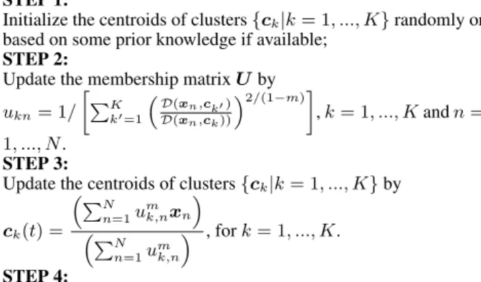
Table 1. The procedure of FCM
STEP 1:
Initialize the centroids of clusters{ck|k= 1, ..., K}randomly or
based on some prior knowledge if available;
STEP 2:
Update the membership matrixUby
ukn= 1/ ! "K k!=1 #D(x n,ck!) D(xn,ck)) $2/(1−m)% ,k= 1, ..., Kandn= 1, ..., N. STEP 3:
Update the centroids of clusters{ck|k= 1, ..., K}by
ck(t) = #"N n=1u m k,nxn $ #"N n=1umk,n $ , fork= 1, ..., K. STEP 4:
RepeatSTEP 2 and 3until!C(t)−C(t−1)!<!, where!is a small positive number.
then-th gene,Mis the number of samples (features or dimensions) andN is the number of genes. Consider that there areKclusters
in a given dataset and each clustering algorithm provides a partition matrixUK×N, where the entryuk,n ∈ [0,1]represents the
mem-bership coefficient ofn-th gene in thekthe cluster.
2.1. Fuzzy Clustering
Fuzzy clustering is a concept that relaxes the restriction of crisp clus-tering, which assigns every object exactly in one clusters, by charac-terizing the membership of each sample point in all the clusters with a membership function which ranges between zero and one. Addi-tionally, the sum of the memberships for each sample point must be unity [4]. The properties of the partition matrix is mathematically expressed by
(a) uk,n∈[0,1], 1≤n≤N,1≤k≤K, (b) "Kk=1uk,n= 1, 1≤n≤N, (c) 0<"Nn=1uk,n< N, 1≤k≤K.
An example of fuzzy clustering is the fuzzy c-means (FCM) [5], which is fuzzy counterpart of the k-means. FCM aims to minimize the cost function, which is mathematically expressed by
J(U,X) = K & k=1 N & n=1 (uk,n)mD(xn,ck), (1)
wherem∈[1,∞)is the fuzzification parameter.D(xn,ck)is the
dissimilarity measure between then-th gene,xn, and the centroid of
thek-th cluster,ck. Similar to k-means, the cost function (1) can be
minimised with an iterative procedure that updates the partition ma-trix and the centroids of clusters alternately. Since many genes may participate in more than one function in the biological process, the fuzzy clustering has obvious advantage to identify some genes co-regulating with more than one cluster of genes. Many applications of FCM and its enhancements and modifications for gene expres-sion data have been developed [6–10]. The procedure of FCM is summarized in Table 1. There are also many other fuzzy clustering approaches, for example, fuzzy self-organizing map (FSOM) [11], fuzzy adaptive resonance theory (FART) [12] and fuzzy support vec-tor machine (FSVM) [13].
2.2. Kernel-based Clustering
Kernel-based clustering, which shares similar idea with support vec-tor machines (SVM), constructs a hyperplane to separate the pat-terns. These patterns are nonlinearly transformed from a set of non-linearly separable patterns into a higher-dimensional feature space to be linear separable [14, 15]. At the core of the kernel-based clus-tering lies the difficulty of explicitly constructing the nonlinear map-ping,Φ(·), which is sometime infeasible; but now it can be overcome
by a kernel trick. The kernel trick is a way of mapping patterns from a input space into a feature space without having to compute the mapping explicitly, in the hope that the patterns will gain meaning-ful linear structure in the feature space, mathematically expressed as
κ(xi,xj) =Φ(xi)TΦ(xj), (2)
where(·)Tis the transpose operator. Thus, a straightforward way to
transform the calculation of Euclidean distance in the feature space into the kernel version is to use the kernel trick as follows
DEκ(Φ(xi),Φ(xj)) = !Φ(xi)−Φ(xj)!2 (3) = !Φ(xi)!2+!Φ(xj)!2−2Φ(xi)TΦ(xj) = κ(xi,xi) +κ(xj,xj)−2κ(xi,xj),
and the kernel version of modified Pearson correlation is given by [16] SPκ(Φ(xi),Φ(xj)) = Φ(xi)TΦ(xj) ' Φ(xi)TΦ(xi)'Φ(xj)TΦ(xj)(4) = ' κ(xi,xj) κ(xi,xi) ' κ(xj,xj) .
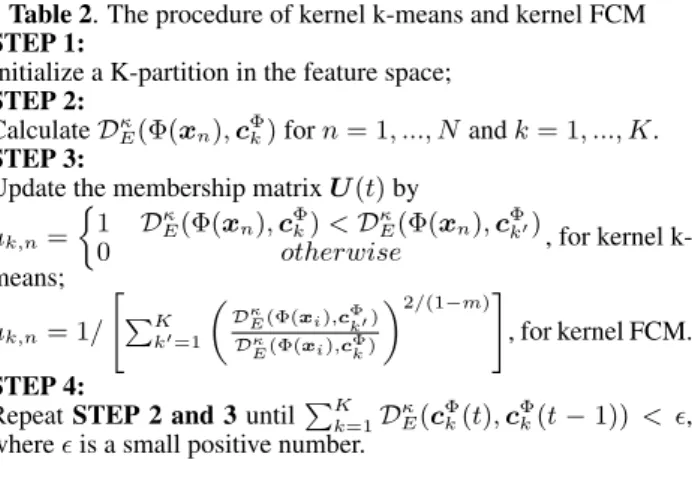
Kernel means (or kernel FCM) is kernel counterpart of the k-means (or FCM) [17], whose core part is to calculate the distance between the objects and the centroids of clusters in the feature space
DEκ(Φ(xi),cΦk) = !Φ(xi)− 1 Nk N & l=1 umk,lΦ(xl)!2 (5) = κ(xi,xi)− 1 Nk N & l=1 umk,lκ(xi,xl) + 1 N2 k N & l=1 N & n=1 umk,lumk,nκ(xl,xn),
whereNk = "Nl=1umkl. For crisp kernel k-means, the elements
in partition matrix are either zero or one andm = 1; for the ker-nel FCM, the partition matrix is the one described in Sec. 2.1 and
m ∈ [1,∞). The procedure of kernel k-means and kernel FCM is summarized in Table 2. Other kernel-based algorithms including kernel hierarchical and kernel principle component analysis can be found in [16, 18].
2.3. Self Organizing Clustering
The Kohonen self-organizing map (SOM) is one of the most popular unsupervised clustering algorithms [19, 20] and has been reviewed in many references [2, 3]. There is another algorithm, called self-organizing oscillator networks (SOON) [21], which also belongs to self-organizing clustering family. The so-called self-organizing means that all the prototypes are attracted to the input patterns in an adaptive fashion. Here, we focus on the SOON algorithm, which
Table 2. The procedure of kernel k-means and kernel FCM
STEP 1:
Initialize a K-partition in the feature space;
STEP 2:
CalculateDκ
E(Φ(xn),cΦk)forn= 1, ..., Nandk= 1, ..., K.
STEP 3:
Update the membership matrixU(t)by
uk,n=
(
1 Dκ
E(Φ(xn),cΦk)<DκE(Φ(xn),cΦk!)
0 otherwise , for kernel
k-means; uk,n= 1/ ) "K k!=1 * Dκ E(Φ(xi),cΦk!) Dκ E(Φ(xi),cΦk) +2/(1−m), , for kernel FCM. STEP 4:
RepeatSTEP 2 and 3until"K k=1D
κ
E(cΦk(t),cΦk(t−1)) <!,
where!is a small positive number.
makes use of a biological fact that fireflies flash together exhibiting a synchronized firing in groups that physically close to each other. The basic unit of clustering in SOON is an integrate and fire (IF) oscillator representing each object in the dataset.
Suppose thatO={O1, ...,ON}is a set ofNoscillators, where
each oscillatorOiis characterized by a phaseφiand a state variable si, given by
si=fi(φi), i= 1, ..., K, (6)
where each functionfi : [0,1] &→ [0,1]is smooth. In [21], the
functionf(φ)was
f(φ) = 1 bln
-1 +#eb−1$φ..
Wheneversireaches a threshold atsi = 1, thei-th oscillator fires
and instantaneously reset to zero, following which the cycle repeats. The firing of all other oscillatorsOj(j(=i)can be affected byi-th
oscillator by
sj(t+) =B(sj(t) +!i(φj)), (7)
whereB(·)is a limiting function to guarantee thatsj(t)is confined
to[0,1], mathematically expressed by B(s) = s if0≤s≤1; 0 ifs <0; 1 ifs >1. (8) The coupling strength of the i-th oscillator at a given phase φj,
!i(φj), is the most important concept of the SOON algorithm, math-ematically expressed by !i(φj) = CE ! 1−#D(Oiδ0,Oj) $2% , ifD(Oi,Oj)≤δ0; −CI !#D(Oi,Oj)−δ0 δ1−δ0 $2% , ifδ0<D(Oi,Oj)≤δ1; −CI, otherwise, (9) whereδ0andδ1are limit distances andδ1is set to be five timesδ0.
CEandCIare the maximum excitatory coupling and the maximum
inhibitory coupling, respectively.
To avoid the need to compute and store the pairwise distances between any pair of objects, prototypesβ={β1, ...,βK}are used
to represent clusters of the object in SOON-2, which is summarized in Table 3.
Table 3. The procedure of SOON-2
STEP 1:
Initialize a phasesφirandomly fori= 1, ..., N;
SetK, and initialize the Prototypesβkrandomly fork= 1, ..., K;
STEP 2:
Identify the next oscillator to fire,{Oi:φi= maxjφj};
Identify the close prototype to the oscillatorOi&→βk;
ComputeD(βk,Oj)for∀j∈[1, N];
Bringφito threshold, and adjust other phases
φj=φj+ (1−φi)for∀j∈[1, N];
STEP 3:
forall oscillatorsOj(j(=i)do
Compute state variablesj;
Compute coupling strength!i(φj); Adjust state variablesjusing (7);
Compute compute new phase usingφj=f−1(sj);
end for
Identify synchronized oscillators and reset their phases; Update prototypeβk;
STEP 4:
RepeatSTEP 2 and 3until synchronized group stabilize.
2.4. Self Splitting and Merging Clustering
Self-splitting and merging clustering is an idea in which without set-ting the number of clusters a priori, the algorithm will converge to a partitioning which reveals the true number of clusters and pro-vides fairly accurate clustering results. Recently, some self splitting-merging clustering algorithms have been developed for both gen-eral purpose clustering [22, 23] and gene expression data analysis [24]. A competitive learning paradigm, called one-prototype-take-one-cluster (OPTOC) [22], was proposed in the self-splitting cluster-ing algorithm. There are two advantages of the OPTOC that, firstly, it is not sensitive to initialization, and secondly, in many cases, it is able to find natural clusters. However, its ability to find the natural clusters depends on the determination of suitable threshold, which is difficult [24]. Being aware of the shortcoming of the OPTOC, a self-splitting-merging competitive learning (SSMCL) algorithm [24] based on the OPTOC paradigm was developed for gene expression analysis. The SSMCL initially over-clusters the whole dataset using the OPTOC principle and then merge the groups based on the second order statistical characteristics. However, although the number of clusters can be initially set to any value lager than the number of nat-ural clusters, the SSMCL still needs to set it as close to the number of natural clusters as possible, otherwise, too much computing power will be wasted due to the unnecessary over-clustering and merging. With the similar principle as the SSMCL, over-clustering and merg-ing, a cohesion-based self-merging (CSM) algorithm, which was re-ported in [23] to combine thek-means and hierarchical clustering, also faces the same problem of setting the initial number of clusters. Here, we briefly introduce the OPTOC competitive learning paradigm. For each prototype, an online learning vecoter called asymptotic property vector (APV), Ak, is assigned to guide the learning thek-th prototypePk. The APV is adapted according to
Ak=Ak+ 1 nk A ·δk·(xn−Ak)Θ(Pk,Ak,xn), (10) where nkA = nkA+δk·Θ(Pk,Ak,xn), Θ(a,b,c) = ( 1 ifD(a,b)≤D(a,c) 0 otherwise , (11)
and δk= ! D(Pk,Ak) D(Pk,xn) +D(Pk,Ak) % . (12)
The learning process forPkis given by
Pk=Pk+αk·(xn−Pk)Θ(Pk,Ak,xn) (13) where αk= ! 1 +D(Pk,xn) D(Pk,Ak) %−2 . (14)
The above OPTOC competitive learning paradigm is an effective technique to implement the self splitting and merging clustering.
2.5. Ensemble Consensus Clustering
Robustness is one of the desired properties of clustering algorithms, However, there is no perfect method which always gives the best results for all types of datasets. In order to enhance the robustness of clustering, the idea of ensemble consensus clustering has been proposed where the partitioning results of many clustering experi-ments are combined [25–33]. These partitioning results may come from different clustering algorithms, or same clustering algorithm with different parameters and initializations, or same clustering al-gorithm to different re-sampled permutations of the target dataset.
Although cluster ensembles have been regarded as promising methods, many obstacles have been found while combining results from different experiments. Due to the fact that clustering is unsu-pervised, one main problem is that it is not a straightforward task to map a specific cluster from one of the clustering results to its corre-sponding cluster from another clustering result. Another problem is that different clustering results may give different numbers of clus-ters while the correct number of clusclus-ters in unknown.
Consensus function method has been employed as an essential step in cluster ensembles. ForRpartitions{U1, ...,UR}, the
opti-mal consensus partitionU∗is the one which is the most similar to
all of them and is mathematically given by
U∗= arg max ∀P R & j=1 Γ(U,Uj) (15) whereΓ(·,·) measures the similarity between any two partitions. This optimization problem has been noted as an NP-complete prob-lem. There are many methods for consensus function, including relabelling and voting [33], co-association matrix [34], hyper-graph methods [25], weighted kernel consensus functions [31], non-negative matrix factorization [32], greedy algorithms [27],
etc. In all of the aforementioned methods, there are at least three steps to implement the ensemble consensus clustering as follows:
Partitions generation: R different clustering experiments are
carried out to generateR partitions. The results of these parti-tions are all presented in a consistent form known as the partition matrix.
Relabelling: The clusters in the generated partitions are rela-belled such that the corresponding clusters from different parti-tions are aligned.
Final consensus partition matrix generation: The relabelled partition matrices are ”assembled” to generate the final consen-sus partition matrix.
Among these three steps,RelabellingandFinal consensus par-tition matrix generationare the most essential parts. An example of relabelling is detailed in the steps below:
(a) A dissimilarity distance matrixSK×K is constructed by cal-culating the pairwise distance between the rows (clusters) of the matrixUand the rows of the reference matrixUref.
(b)The minimum value in each of the columns is found.
(c) The maximum value of these minima is identified then the rows (clusters) fromUandUrefwhich correspond to this
simi-larity value are mapped.
(d)The row and the column which show the aforementioned value are deleted from the similarity matrix.
(e)If all of theK rows fromU and Uref are mapped, the
al-gorithm terminates, otherwise it goes back to step (2) with the reduced similarity matrix.
It is suggested that an intermediate consensus partition matrix
Uint(k) is initialized with the values of the first partitionU1, and
then the other partitions are relabelled and fused with this interme-diate matrix one by one while considering it as the reference at each step. Mathematically, letUˆr be the relabelled partition matrix of
the partitionUr and letUint(k) be the intermediate partition
ma-trix after the k-th stage, i.e. after relabelling and fusing the parti-tions{U1,
· · ·,Uk
}. Let the function Relabel(U,Uref) denote
relabelling the partition matrix U by consideringUref as the
ref-erence partition. Equation (3) shows how the intermediate partition matrix can be calculated by the normal approach and the recursive approach: Uint(k)= 1 k k & r=1 ˆ Ur= 1 kUˆ k +(k−1) k U int(k−1). (16)
An example of generating the final consensus partition ma-trix is achieved by following the algorithm shown in the following steps: (1)Uint(1)=U1 (2) Fork= 2toR a.Uˆk=Relabel(Uk,Uint(k−1)) b.Uint(k)= 1 kUˆ k +k−1 k U int(k−1) (3)U∗=Uint(R). 3. CLUSTERING VALIDATION
Since clustering is unsupervised classification, it is more difficult to assess than a supervised approach. Thus, the task of assessing the results of clustering algorithms can be as important as the clus-tering algorithms themselves. There are two functional advantages of employing the clustering validations: firstly, they can validate a clustering algorithm by comparing with other algorithms; secondly, some validity indices can provide an estimate of the number of clus-ters, which is crucial information for the clustering analysis. In this section, we will review some existing clustering validations.
3.1. Parametric Validity index
A parametric validity index (PVI), which employs two tunable pa-rametersαandβ to to control the proportions of objects that are
involved in the calculation of the intra-cluster dissimilarities and the inter-cluster dissimilarities, was proposed in [35]. For each clus-ter, three spaces are defined, namely the inner space, the intra outer space and the inter outer space, representing the objects inside the cluster chosen for the calculation of both the intra-cluster dissim-ilarities and the inter-cluster dissimdissim-ilarities, the objects inside the cluster chosen for the calculation of only the intra-cluster dissimi-larities, and the objects outside the cluster chosen for the calculation
of only the inter-cluster dissimilarities, respectively. LetNki,N aok, N eo
kdenote the numbers of objects in the inner space, the intra outer
space and the inter outer space, respectively, for thek-th cluster. The fractions,αandβ, are used to controlNki,N aok,N eok, which can be
expressed as
Nki=*αNk+, N aok=*βNk+, N eok=*β(N−Nk)+, (17)
whereNkis the number of the objects in thek-th cluster,N is the
number of all objects in the dataset and*·+is the ceiling operator. Bothαand β can be chosen from the range of (0,1]. Thus, the inner space isAk = {aak|a = 1, ..., Nk}i , the intra outer space is Ba
k = {ba,bk |b = 1, ..., N aok}, and the inter outer space isCka = {ca,ck |c= 1, ..., N eok}. The PVI is obtained by
PVI(K,α,β) = K & k=1 Nki & a=1 * Dea k Daa k + , (18) where Daak = !N aok b=1 D(aak,b a,b k ) N ao k Deak = !N eok c=1D(aak,c a,c k ) N eo k . (19) 3.2. Other Indices
In this section, we list five other existing validity indices. The first is theVI[36]. The validity indexVI is the ratio of the inter-cluster
separation measures and the intra-cluster scatter measures, which is mathematically expressed as VI(K) = "K i=1Iei "K i=1Iai , (20)
whereKis the number of clusters. TheVIemploysIai, the largest
dissimilarity of the minimum spanning tree (MST) for cluster i, as the intra-cluster scatter andIei = minKj=1,j%=iIeij, whereIeijis
the the largest dissimilarity of the MST for cluster i and cluster j, as the inter-cluster separation.
The second is theDI[37], which is written as
DI(K) = min 1≤i≤K ( min 1≤j≤K ( δ(Ci,Cj) max1≤k≤K{∆(Ck)} 33 , (21) whereδ(Ci,Cj) = min!xi−xj!2 is the maximum distance
be-tween clusteriand clusterj,∆(Ck)is the largest intra-cluster sepa-ration of clusterk. The third is theII[38], which is written as
II(K) = * 1 K × E1 EK × DK +P , (22)
whereE1 = "j!xj−c!2 wherecis the centroid of the whole
dataset,EK = "Kk=1 "
j∈Ck!xj−ck!2,DK = maxKi,j!ci−
cj!2and powerP is constant, which is 2 in our experiments. The
fourth is theGI[39], which is expressed as
GI(K) = max 1≤k≤K 4 (2"Mm=1√λmk)2 min1≤j≤K!ui−uj!2 5 , (23) whereM is the number of dimensions,λmkare the eigenvalues of
the covariance matrix of thek-th cluster. Note that the closestGI
value to zero suggests the best number of clusters. The fifth is the
CH[40] which is given by CH(K) = -!K k=1nk(ck−u(2 K−1 . !!K k=1 !nk i=1(xi−ck(2 n−K %, (24)
wherenkis the number of memberships in the clusterkandnis the
total number of the objects. The performance of above five clustering validations has been compared for gene expression dataset in [41]
4. DATASETS
There have been many benchmark gene expression datasets in the literature. People can either test their new clustering algorithms us-ing these datasets or employ their clusterus-ing algorithms to investi-gate these datasets and provide new points of view in the biological context.
(a) The synthetic data set models gene expression data with cyclic behavior. Classes are modelled as genes that have peak times over the times course as presented in [42, 43].
(b)The leukemia dataset [44] consists of 38 bone marrow sam-ples obtained from acute leukemia patients at time of diagnosis. The samples include 11 acute myeloid leukemia (AML) samples, 8 T-lineage acute lymphoblastic leukemia (ALL) samples and 19 B-lineage ALL samples. There are 999 genes in the dataset.
(c)The yeast cell cycle dataset was published by Choet al.[45]. It consists of more than 6000 genes over 17 time points taken at 10 minutes intervals, where 383 genes were identified and these demon-strated consistent periodic changes in transcript level. It was com-monly believed that the time course was divided into early G1, late G1, S, G2, and M phases, those 383 genes would peak at one of the five phases. In [42], a subset with 384 genes was investigated.
(d)The lymphoma dataset have three most prevalent adult lym-phoid malignancies [46].
(e)The liver cancer dataset is available in [47].
5. CONCLUSIONS AND FUTURE WORK
In this paper, we systematically reviewed five clustering families rep-resenting five different clustering concepts. We also reviewed some clustering validations and collected a list of benchmark gene expres-sion datasets. We are implementing algorithms in all of the afore-mentioned clustering families and investigating their performance in all of listed benchmark gene expression datasets. The performance comparison and validation will be presented in a future publication and the forthcoming conference.
6. REFERENCES
[1] D. M. Dziuda, Data Mining for Genomics and Proteomics: Analysis of Gene and Protein Expression Data, Wiley, 2010.
[2] R. Xu and D. II Wunsch, “Survey of clustering algorithms,” IEEE Trans. Neural Networks, vol. 16, no. 3, pp. 645 – 678, 2005. [3] D. X. Jiang, C. Tang, and A. D. Zhang, “Cluster analysis for gene
expression data: A survey,” IEEE Trans. Know. and Data Eng., vol. 16, no. 11, pp. 1370–1386, 2004.
[4] Bezdek, Pattern recognition with fuzzy objective function algorithms, New York: Plenum, 1981.
[5] James C. Bezdek, Robert Ehrlich, and William Full, “FCM: The fuzzy c-means clustering algorithm,”Comput. Geosoci, vol. 10, no. 2-3, pp. 191 – 203, 1984.
[6] M.E. Futschik and N.K. Kasabov, “Fuzzy clustering of gene expression data,” inProc. IEEE Int. Conf. Fuzzy Systems, FUZZ-IEEE’02, 2002, vol. 1, pp. 414 –419.
[7] Doulaye Dembl and Philippe Kastner, “Fuzzy c-means method for clustering microarray data,”Bioinformat., vol. 19, no. 8, pp. 973–980, 2003.
[8] J. W. Luo, T. Yang, and Y. Wang, “Missing value estimation for mi-croarray data based on fuzzy c-means clustering,” inProc. Eighth Int. Conf. High-Perf. Computing in Asia-Pacific Region, 2005.
[9] Sanghamitra Bandyopadhyay, Anirban Mukhopadhyay, and Ujjwal Maulik, “An improved algorithm for clustering gene expression data,” Bioinformat., vol. 23, no. 21, pp. 2859–2865, 2007.
[10] Luis Tari, Chitta Baral, and Seungchan Kim, “Fuzzy c-means cluster-ing with prior biological knowledge,” J. Biomed. Informat., vol. 42, no. 1, pp. 74 – 81, 2009.
[11] R.D. Pascual-Marqui, A.D. Pascual-Montano, K. Kochi, and J.M. Carazo, “Smoothly distributed fuzzy c-means: a new self-organizing map,”Pattern Recognition, vol. 34, no. 12, pp. 2395 – 2402, 2001. [12] Shuta Tomida, Taizo Hanai, Hiroyuki Honda, and Takeshi Kobayashi,
“Analysis of expression profile using fuzzy adaptive resonance theory,” Bioinformat., vol. 18, no. 8, pp. 1073–1083, 2002.
[13] Y. Mao, X. B. Zhou, D. Y. Pi, Y. X. Sun, and Stephen T. C. Wong, “Multiclass cancer classification by using fuzzy support vector ma-chine and binary decision tree with gene selection,” J. Biomed. Biotech., vol. 2005, no. 2, pp. 160–171, 2005.
[14] K.-R. Muller, S. Mika, G. Ratsch, K. Tsuda, and B. Scholkopf, “An introduction to kernel-based learning algorithms,”IEEE Trans. Neural Networks,, vol. 12, no. 2, pp. 181 –201, 2001.
[15] Michael P. S. Brown, William Noble Grundy, David Lin, Nello Cris-tianini, Charles Walsh Sugnet, Terrence S. Furey, Manuel Ares, and David Haussler, “Knowledge-based analysis of microarray gene ex-pression data by using support vector machines,”Proc. Nat. Academy Sci., vol. 97, no. 1, pp. 262–267, 2000.
[16] Jie Qin, Darrin P. Lewis, and William Stafford Noble, “Kernel hierar-chical gene clustering from microarray expression data,”Bioinformat., vol. 19, no. 16, pp. 2097–2104, 2003.
[17] Inderjit S. Dhillon, Yuqiang Guan, and Brian Kulis, “Kernel k-means: spectral clustering and normalized cuts,” inProc. Tenth ACM SIGKDD Int. Conf. Know. disc. data mining, New York, NY, USA, 2004, KDD ’04, pp. 551–556, ACM.
[18] Z. G. Liu, D. C. Chen, and H. Bensmail, “Gene expression data classification with kernel principal component analysis,” J. Biomed. Biotech., vol. 2005, no. 2, pp. 155–159, 2005.
[19] T. E. Kohonen, Self-Organizing Maps,, New York: Springer-Verlag, 1997.
[20] P. Tamayo, D. Slonim, J. Mesirov, Q. Zhu, S. Kitareewan, E. Dmitro-vsky, E. S. Lander, and T. R. Golub, “Interpreting patterns of gene expression with self-organizing maps: Methods and application to hematopoietic differentiation,”Proc. Nat. Academy Sci. USA, vol. 96, no. 6, pp. 2907–2912, 1999.
[21] Sameh A. Salem, Lindsay B. Jack, and Asoke K. Nandi, “Investigation of self-organizing oscillator networks for use in clustering microarray data,”IEEE Trans. NanoBio., vol. 7, no. 1, pp. 65–79, 2008. [22] Ya-Jun Zhang and Zhi-Qiang Liu, “Self-splitting competitive learning:
a new on-line clustering paradigm,”IEEE Trans. Neural Networks, vol. 13, no. 2, pp. 369 –380, mar 2002.
[23] Cheng-Ru Lin and Ming-Syan Chen, “Combining partitional and hier-archical algorithms for robust and efficient data clustering with cohe-sion self-merging,”IEEE Trans. Know. Data Eng., vol. 17, no. 2, pp. 145 – 159, 2005.
[24] Shuanhu Wu, A.W.-C. Liew, Hong Yan, and Mengsu Yang, “Cluster analysis of gene expression data based on self-splitting and merging competitive learning,” IEEE Trans. Inf. Tech. Biomed., vol. 8, no. 1, pp. 5 –15, 2004.
[25] A. Strehl and J. Ghosh, “Cluster ensembles C a knowledge reuse framework for combining multiple partitions’,,”J. Machine Learning Research,, vol. 3, pp. 583–617, 2002.
[26] Stefano Monti, Pablo Tamayo, Jill Mesirov, and Todd Golub, “Con-sensus clustering: A resampling-based method for class discovery and visualization of gene expression microarray data,”Machine Learning, vol. 52, pp. 91–118, 2003.
[27] V. Filkov and S. Skiena, “Integrating microarray data by consensus clustering,” inProc. Int. Conf. Tools with Art. Intell., pp. 418–426, 2003.
[28] Xiaohua Hu and Illhoi Yoo, “Cluster ensemble and its applications in gene expression analysis,” inProc. Second Conf. Asia-Pacific bioin-format., APBC’04,- v. 29, pp. 297–302, Australian Computer Society. [29] Stephen Swift, Allan Tucker, Veronica Vinciotti, Nigel Martin, Chris-tine Orengo, Xiaohui Liu, and Paul Kellam, “Consensus clustering and functional interpretation of gene-expression data,” Genome Biol-ogy, vol. 5, no. 11, pp. R94, 2004.
[30] R. Avogadri and G. Valentini, “Ensemble clustering with a fuzzy ap-proach,” Studies in Comput. Intell. Superv. and Unsuperv. Ensemble Methods their Appl., v. 126, pp 49-69, 2008.
[31] S. Vega-Pons, J. Correa-Morris, and J. Ruiz-Shulcloper, “Weighted cluster ensemble using a kernel consensus function,” Lecture Notes in Computer Science, Heidelberg: Springer., vol. 5197, pp. 195–202, 2008.
[32] W. Wang, “An improved non-negative matrix factorization algorithm for combining multiple clusterings,” in2010 Int. Conf. Machine Vision Human-machine Interface, pp. 604–607, 2010.
[33] H. G. Ayad and M. S. Kamel, “On voting-based consensus of cluster ensembles,”Pattern Recognition, vol. 43, pp. 1943-C1953, 2010. [34] A. Fred and A. K. Jain, “Data clustering using evidence
accumula-tion’,,” inProc. Sixteenth Int. Conf. Pattern Recognition (ICPR), pp. 276–280, 2002.
[35] R. Fa and A. K. Nandi, “Parametric validity index of clustering for microarray gene expression data,” inIEEE Int. Workshop Machine Learning for Sig. Process. 2011 (MLSP 2011), 2011.
[36] Sameh A. Salem and Asoke K. Nandi, “Development of assessment criteria for clustering algorithms,”Pattern Anal. and Appl., vol. 12, no. 1, pp. 79–98, 2009.
[37] J. C. Dunn, “A fuzzy relative of the isodata process and its use in detecting compact well-separated clusters,”J. Cyber., vol. 3, no. 3, pp. 32–57, 1973.
[38] U Maulik and S Bandyopadhyay, “Performance evaluation of some clustering algorithms and validity indices,”IEEE Trans. Pattern Anal. Mach. Intell., vol. 24, no. 12, pp. 1650–1654, 2002.
[39] Benson S. Y. Lam and Hong Yan, “Assessment of microarray data clustering results based on a new geometrical index for cluster valid-ity,”Soft Computing, vol. 11, no. 4, pp. 341–348, 2007.
[40] T. Calinski and J. Harabasz, “A dendrite method for cluster analysis,” Communications in Statistics - Theory and Methods, vol. 3, no. 1, pp. 1–27, 1974.
[41] R. Fa and A. K. Nandi, “Comparisons of validation criteria for cluster-ing algorithms in microarray gene expression data analysis,” inProc. Second Int. Workshop Genomic Signal Process. (GSP2011), 2011. [42] K. Y. Yeung, C. Fraley, A. Murua, A. E. Raftery, and W. L. Ruzzo,
“Model-based clustering and data transformations for gene expression data,”Bioinformat., vol. 17, no. 10, pp. 977–987, 2001.
[43] L. P. Zhao, R. Presntice, and L. Breeden, “Statistical modelling of large microarray data sets to identify stimulus-response profiles,”Proc. Natl. Acad. Sci. (PNAS), vol. 98, no. 10, pp. 5631–5636, 2001.
[44] T. R. Golub, D. K. Slonim, P. Tamayo, C. Huard, M. Gaasenbeek, J. P. Mesirov, H. Coller, M. L. Loh, J. R. Downing, M. A. Caligiuri, C. D. Bloomfield, and E. S. Lander, “Molecular classification of cancer: Class discovery and class prediction by gene expression monitoring,” Science, vol. 286, no. 5439, pp. 531–537, 1999.
[45] R. J. Cho, M. J. Campbell, E. A. Winzeler, L. Steinmetz, A. Conway, L. Wodicka, T. G. Wolfsberg, A. E. Gabrielian, D. Landsman, D. J. Lockhart, and R. W. Davis, “A genome-wide transcriptional analysis of the mitotic cell cycle,”Mol. Cell, vol. 2, no. 1, pp. 65–73, 1998. [46] Alizadeh et al., “Distinct types of diffuse large b-cell lymphoma
iden-tified by gene expression profiling,” 2000, Nature, 403(6769):pp. 503– 511. http://llmpp.nih.gov/lymphoma/index.shtml.
[47] Chen X et al., “Gene expression patterns in human liver cancers,” 2002, Mol. Biol. Cell 13(6): pp. 1929–1939 , http://www.ncbi.nlm.nih.gov/, GSE3500 record.