High-Dimensional Behavior of Some Multivariate Two-Sample Tests

High-Dimensional Behavior of Some

Multivariate Two-Sample Tests

Shan Shi

A Thesis

for The Department of

Mathematics and Statistics

Presented in Partial Fulfillment of the Requirements

for the Degree of Master of Arts (Mathematics) at

Concordia University

Montreal, Quebec, Canada

November 2015

c

CONCORDIA UNIVERSITY

School of Graduate Studies

This is to certify that the thesis prepared

By:

Shan Shi

Entitled:

High-Dimensional Behavior of Some Multivariate

Two-Sample Tests

and submitted in partial fulfillment of the requirements for the degree of

Master of Arts (Mathematics)

complies with the regulations of the University and meets the accepted

standards with respect to originality and quality.

Signed by the final examining committee:

Examiner

Dr. Wei Sun

Examiner

Dr. Yogendra Chaubey

Thesis Supervisor

Dr. Arusharka Sen

Approved by

Chair of Department or Graduate Program Director

Dean of Faculty

ABSTRACT

High-dimensional behavior of some multivariate two-sample tests

Shan Shi

It is a difficult problem to test the equality of distribution of two independent p-dimensional (p >1) samples (of sizes m andn, say) in a nonparametric framework. It is not only because we need deal with issues such as tractability of the null distribution of test-statistics but also the fact that the latter are rarely distribution-free. Several notable nonparametric tests for comparing multivariate distributions are the multivariate runs test of Friedman and Rafsky (1979), the nearest-neighbor test of Henze (1988) and the inter-point distance-based test of Baringhaus and Franz (BF) (2004). Biswas and Ghosh (BG) (2014) recently have shown that in a high dimension, low sample-size (HDLSS) scenario, i.e. wherep goes to infinity butm, n

are small or fixed, all the tests mentioned do not perform well. However, the BG-test is shown to be consistent in the case of HDLSS. In this work, we study the asymptotic behaviors of BF and BG tests when m, n and pgo to infinity and min(m, n) =o(p). Our results reveal when these tests are expected to work well and when they are not. Results are illustrated by simulated data.

Acknowledgments

I’d like to express my sincere gratitude to my supervisor Dr. Arusharka Sen for all his supports and help throughout my Master’s degree. And, I want to thank you to all of the wonderful professors at Concordia University who have helped me to broaden my knowledge in math and encouraged me to pursue my passion for academic research. I would also like to thank Dr. Wei Sun and Dr. Yogendra Chaubey for reviewing my thesis.

Contents

List of Figures vii

Introduction 1

0.1 High-Dimensional Data Problems . . . 1

0.2 Hypothesis Testing For Distributions . . . 2

0.3 U₋Statistics . . . 5

0.4 Thesis Organization . . . 6

1 Behavior of the BF-test as m, n, p _{→ ∞} 7 1.1 Assumptions . . . 7 1.2 Taylor Approximation ofTBF∗ mn . . . 8 1.3 Asymptotic normality ofTBF∗ mn Under H0 . . . 10 1.4 Ratio-Consistent Estimators . . . 15

2 Behavior of the BG-test as m, n, p_{→ ∞} 17 2.1 Taylor Approximation of N_pTBG mn . . . 17

2.2 Asymptotic distribution of N_pTmnBG . . . 18

2.3 A ratio consistent estimator forV₍N pT BG mn) . . . 20

2.4 Power properties of the BG-test . . . 25

3 Simulation Results 27 3.1 Simulation of Power curves . . . 27

List of Figures

3.1 Power curves of BF-test . . . 28 3.2 Power curves of BG-test in the case of HDLSS . . . 30 3.3 Power curves of BG-test . . . 31

Introduction

Classical statistical data analyses can only be applied in the case where the dimension of observations is fixed and the sample size grows. In many recent practical applications, such as data mining and microarray studies, we face a new challenge that is the number of variables exceeds the number of observations dramatically. Due to the growing dimension of data, many classical statistical data analysis tool are not available any more.

0.1

High-Dimensional Data Problems

In order to show some challenges happening in high-dimensional settings, let’s consider two random samples X1, X2, . . . , Xm andY1, Y2, . . . , Yn, whereXi, Yj ∈Rp, for all 1≤i, j ≤m, n. Now, let µ1 = E(Xi), µ2 = E(Yj) where µ1 = (µ11, µ12, . . . , µ1p)0, µ2 = (µ21, µ22, . . . , µ2p)0 and the covariance matrices Σ1 =cov(Xi), Σ2 =cov(Yj). Let’s assume we are interested in

testing

H0 :µ1 =µ2 vs. H1 :µ1 6=µ2.

Traditionally, the Hotteling T2 _{test is a widely used mean test. The test statistic is defined}

as follow

T2 = mn

m+n X¯ −Y¯

S_N−1 X¯ ₋Y¯

where N =m+n, ¯X,Y¯ are sample mean vectors andSN is the pooled sample covariance matrix defined as SN = 1 m+n₋2 " _m X i=1 Xi−X¯ Xi−X¯ 0 + n X j=1 Yj−Y¯ Yj−Y¯ 0 # .

Under the null hypothesis, N−_{N p}p+1T2 _{has a central F-distribution with p and N −p + 1}

degrees of freedom. However, Bai and Saranadasa (1996) show that the asymptotic power of Hotelling’s test decrease as the ratio of the dimension to the sample size, p/N, increases to 1. When p > N, that is, the dimension is larger than the sample size, the Hotelling’s test is not well defined because the sample covariance matrix becomes singular. Thus, Bai and Saranadasa (1996) proposed replacing ( ¯X₋Y¯)0

S_N−1( ¯X₋Y¯) in the Hottelling’s test with

kX¯ ₋Y¯_k, where _{k · k}denotes the Euclidean norm. The test statistic they established, under some mild conditions, shows attractive power as p/n_→c <_∞.

0.2

Hypothesis Testing For Distributions

The high-Dimensional challenges also arise in problems of two-sample hypothesis testing for distributions. Before we proceed, let’s have a short review on two-sample hypothesis testing for distributions. In such tests, we are interested in either H0 : F = G or H1 : F 6= G. In

other words, we would like to know if two sets of independent observationsXi ∼F,1≤i≤m and Yj ∼G,1≤j ≤n share the same distribution function. The two-sample test problem has been studied for a long time in fixed dimension settings. In the univariate case, some distribution-free and consistent tests such as the Kolmogorov-Smirnov, Wald-Wolfowitz runs and Wilcoxon rank sum tests are commonly applied. However, the multivariate case seems not as straightforward as the univariate case. The easily noticed reason is the fact that the multivariate tests often are not distribution-free under H0. Notable among many

proposals for test-statistics are the multivariate runs test of Friedman and Rafsky (1979), the nearest-neighbor test of Henze (1988) and the inter-point distance-based test of Baringhaus and Franz (2004).

Baringhaus and Franz (2004) proposed the test for arbitrary dimensions setting, which is based on the average sample Euclidean inter-point distances, where

T_m,nBF = mn m+n " 1 mn m X j=1 n X k=1 kXj−Ykk − 1 2m2 m X j=1 m X k=1 kXj −Xkk − 1 2n2 n X j=1 n X k=1 kYj−Ykk # ,

the fact proven by Baringhaus and Franz (2004)

2E_(kX−Yk)−E_(kX−X∗_k)−E_{(kY −Y}∗_k)≥0

where X, X∗ i.i.d_{∼ F, Y, Y}∗ i.i.d_{∼ G and the equality holds if and only if F = G. The null}

hypothesis will be rejected when TBF

m,n is large. And, Tm,nBF converges in distribution to an integrated, squared Brownian bridge depending on an unknown distribution, where the theorem is the following.

Theorem 0.2.1. Let X1, X2, . . . , Y1, Y2, . . . be independent p-dimensional random vectors.

They have the same distribution function H. Then, as min(m, n)_{→ ∞}, the random variables

Tm,n converge in distribution to

T =γp

Z

B_H2 (a, t)dµ_⊗λ(a, t),

where (BH(a, t); (a, t)∈Sp−1×R) is a H-Brownian bridge having the covariance function

Cov(BH(a, t), BH(b, s)) =P(a0X1 ≤t, b0X1 ≤s)−P(a0X1 ≤t)P(b0X1 ≤s)

with (a, t),(b, s)_∈Sp−1_×R.

Since BF-test depends on an unknown distribution the authors suggested to simulate critical values by using the bootstrap method.

Recently, Biswas and Ghosh (2014) have demonstrated that in a high dimension, low sample-size (HDLSS) scenario, i.e., where p_{→ ∞} butm, n are small, all the tests mentioned above exhibit poor power. So, they proposed another test related to BF-test. The BG-test statistic is TBG m,n =kµˆDF −µˆDGk2, where ˆ µDF = " ˆ µF F = m 2 −1_Xm i=1 m X j=i+1 kXi−Xjk, µˆF G= (mn)−1 m X i=1 n X j=1 kXi−Yjk # , ˆ µDG= " ˆ µF G= (mn)−1 m X i=1 n X j=1 kXi−Yjk, µˆGG= n 2 −1_Xn i=1 n X j=i+1 kYi−Yjk # .

Like BF-test, the null hypothesis will be rejected when TBG

m,n is large. The BG-test works because, if we let µF F = E(kX−X∗k), µGG = E(kY −Y∗k), µF G = E(kX−Yk), µDF = (µF F, µF G)0, µDG= (µF G, µGG)0, then

kµDF −µDGk2 = 0 ⇔µDF =µDG⇔µF F =µGG =µF G

⇔2µF G−µF F −µGG= 0⇔F =G.

The motivation is they observed that in a high dimension, low sample-size (HDLSS) scenario, the BF-test has bad performances only when v2 _{≤ |σ}2

1−σ22|, whereσ12 = lim_p →∞ trace(Σ1) p , σ 2 2 = lim p→∞ trace(Σ2) p , v2 = lim_p→∞k µ1−µ2k2

p , and Σ1 =Cov(Xi), Σ2 =Cov(Yj),µ1 =E(Xi), µ2 =E(Yj), 1_≤i, j _≤m, n. The authors realized the factv2 _{≤ |σ}2

1 −σ22|implies, assuming σ1 ≤σ2 √ 2σ1 ≤ q σ2 1 +σ22+v2 ≤ √ 2σ2.

And, according to their assumptions, (ˆµF G−µˆF F) √_p →p ( p σ2 1 +σ22+v2− √ 2σ1) and (ˆµF F√−_pµˆGG) →p (pσ2 1+σ22+v2− √

2σ2). Even when (ˆµF G−µˆF F) and (ˆµF F−µˆGG) may be significantly differ-ent from zero, both most likely have differdiffer-ent signs. Thus,TBF

m,n = (ˆµF G−µˆF F) + (ˆµF F−µˆGG) might be close to zero, so H0 may not be rejected. Tm,nBG does not have the same weakness since the cancellation is impossible to happen when TBG

m,n = (ˆµF G−µˆF F)2+ (ˆµF F −µˆGG)2. When sample size is large and the dimension of data remains fixed, (m+n)TBG

m,n converge in distribution to 2σ02 λ(1−λ)χ 2 1, where λ= mn, σ 2

0 = V(E(kX1−X2k|X1)). While the sample size is

fixed and the dimension of data increases, the power of the BG-test of level α converges to 1 if limp_→∞ kµ1−µ2k2 p 6= 0 or limp→∞ trace(Σ1) p 6= limp→∞ trace(Σ2) p is assumed.

It is easy to note that both BF-test and BG-test are linear combinations of U₋Statistics, which is a very powerful tool and has been widely employed since 1948 when Hoeffding first introduced it to the world. Recently, people have attempted to use the asymptotic theory of U₋ statistics especially in the degenerating case to tackle high-dimensional problems. However, Ahmad et al. (2014), claimed that no mentionable bibliography indicated that the asymptotic theory of degenerate U₋statistics was successfully applied to high-dimensional problems. But, Ahmad et al. (2014) proposed a way to apply degenerate U-statistics theory

on high-dimensional problems without explicit proof. In this work, following Jung, Sen and Marron (2012), we are going to simplify Ahmad et al. (2014)’s method by using principal components. We therefore review some basic definitions and theorems of U-statistics.

0.3

U

₋

Statistics

Let X1, X2, X3, . . . be i.i.d random variables with common distribution function F(x). let

m_≥1 andh :Rm _{→Rbe a measurable function symmetric in its arguments. TheU-statistic} with kernel h is defined by

Un(h) = n m −1 _X 1≤i1<i2<···<im≤n h(Xi1, . . . , Xim), n≥m.

The kernel h is called degenerate with respect to F(x) if for all 1_≤j _≤m,

Z

R

h(x1, x2, . . . , xm)dF(xj) = 0, where − ∞< x1, . . . , xj−1, xj+1, . . . , xm <∞.

Let

θ =E_{h(X1, . . . , Xm)}

and for i= 0. . . , m let

hi(x1, . . . , xi) =Eh(x1, . . . , xi, Xi+1, . . . , Xm)

σ_i2 =V_{(hi(X1, . . . , Xi))}

so that

σ₀2 = 0

σ_m2 =V_{(h(X1, . . . , Xm))}

We say that a U-statistic is degenerate if σ2 1 = 0.

Theorem 0.3.1. Let Un be a U-statistic based on a kernel function h of degree m, then V_{(Un) =} n m −1_Xm i=1 m i n₋m m₋i σ2_i

0.4

Thesis Organization

In this work, we will show how BF-test and BG-test behave in the high dimensional setting where n, p _{→ ∞} and n = o(p). In Chapter 1 and 2 the asymptotic distributions of the test statistics of BF-test and BG-test under the null hypothesis and theirs power properties respectively are given. In Chapter 3, a comparison between BF and BG tests would be made.

Chapter 1

Behavior of the BF-test as

m, n, p

_{→ ∞}

The goal of this chapter is to show how BF-test behaves in the case of the high-dimensional setting. Instead of analyzing the original BF-test, we would like to work on the modified BF-test. Its test statistic is

T_m,nBF∗ = (m+n) " 2Pm_j=1Pn_k=1kXj−Ykk mn − Pm j=1 Pm k=1kXj−Xkk m(m₋1) − Pn j=1 Pn k=1kYj −Ykk n(n₋1) # .

To do the investigation, we need first find out the main contributors of TBF∗

m,n by analyzing its Taylor approximation. Then, we would derive its limiting distribution under H0.

1.1

Assumptions

In order to carry out the investigation on these two tests, we need first to make the following assumptions, following Hall and Neeman (2005) and Biswas and Ghosh (2014).

(A1) The fourth moments of the components of X and Y are uniformly bounded, where

X, Y _∈Rp_. (A2) (i) trace(Σ1) p →σ21,(ii) trace(Σ2) p →σ22,(iii) k µ1−µ2k2 p →v2,(iv) trace(ΣiΣj) p2 →cij,asp→ ∞ wherei, j = 1,2.

(A3) X = (X(1)_{, X}(2)_{, . . . , X}(p)_{), Y = (Y}(1)_{, Y}(2)_{, . . . , Y}(p)_{) are ρ mixing for functions}

g(u, v)_{| ≤}Cu2_v2_{, for some C >0, and all u, v, we have}

sup

1≤l,k<∞,|k−l|≥r|

corrf(U(k), V(k)), g(U(l), V(l))_{| ≤}ρ(r),

for (U, V) = (X, X),(Y, Y),(X, Y)

As a consequence of the assumptions, we will have the following

(i) _kXi−Xj p k →p √ 2σ1,(ii)k Yi−Yj p k →p √ 2σ2,(iii) k Xi−Yj p k →p q σ2 1+σ22+v2

since the variances of them go to zero asp goes to infinity. For more details, please refer to Hall and Neeman (2005).

1.2

Taylor Approximation of

T

The way to show how BF-test behaves is to find the main contributors of the test statistic. So, let’s begin with the Taylor expansion of TBF∗

m,n . By simple calculation, we know

µx p = E_(kXi−Xjk2₎ p = 2trace(Σ1) p ≈2σ 2 1 µy p = E_{(kYi −Yjk}2₎ p = 2trace(Σ2) p ≈2σ 2 2 µxy p = E_(kXi−Yjk2₎ p = trace(Σ1+ Σ2) p + kµ1−µ2k2 p ≈σ 2 3 =σ21+σ22+v2

expansions of the functionx_→√x centering at σ2 1, σ22, σ33 ˆ µF F √_p = 2 m(m₋1) m X i=1 m X j=i+1 kXi−_p Xjk =√2σ1+ 1 m√2σ1 m X i=1 (Xi−µ1) 0 (Xi−µ1) p −σ 2 1 ! − 2 m(m₋1)√2σ1 m X i=1 m X j=i+1 (Xi−µ1) 0 (Xj−µ1) p +RµF F ˆ µGG √_p = 2 n(n₋1) n X i=1 n X j=i+1 kYi−_p Yjk =√2σ2+ 1 n√2σ2 n X i=1 (Yi−µ2) 0 (Yi−µ2) p −σ 2 2 ! − 2 n(n₋1)√2σ2 n X i=1 n X j=i+1 (Yi−µ2) 0 (Yj −µ2) p +RµGG ˆ µF G √_p = 1 mn m X i=1 n X j=1 kXi−Yj p k =σ3+ 1 2mσ3 m X i=1 (Xi−µ1) 0 (Xi−µ1)−pσ21 p + 1 2nσ3 n X i=1 (Yi−µ2) 0 (Yi−µ2)−pσ22 p − 1 mnσ3 m X i=1 n X j=1 (Xi−µ1) 0 (Yj −µ2) p − _mnσ1 3 m X i=1 n X j=1 ((Xi−µ1)−(Yj −µ2)) 0 (µ1−µ2) p + 1 2σ3 kµ1−µ2k2 p −v 2 +RµF G

Thus, the modified BF-test can be expressed as the following TBF∗ m,n √_p = (m+n) (2σ3−σ1−σ2) + (m+n) 1 2σ3 kµ1−µ2k2 p −v 2 (1.1) + (m+n)( 2 m(m₋1)√2σ1 m X i=1 m X j=i+1 (Xi−µ1) 0 (Xj −µ1) p (1.2) + 2 n(n₋1)√2σ2 n X i=1 n X j=i+1 (Yi−µ2) 0 (Yj−µ2) p (1.3) − _mnσ2 3 m X i=1 n X j=1 (Xi−µ1) 0 (Yj−µ2) p (1.4) + ( 1 mσ3 − 1 m√2σ1 ) m X i=1 (Xi−µ1) 0 (Xi−µ1)−pσ12 p (1.5) + ( 1 mσ3 − 1 n√2σ2 ) n X i=1 (Yi−µ2) 0 (Yi−µ2)−pσ22 p (1.6) − _mnσ1 3 m X i=1 n X j=1 ((Xi −µ1)−(Yj−µ2)) 0 (µ1−µ2) p (1.7) + 2RµF G−RµF F −RµGG) (1.8)

The term (1.1),(1.5),(1.6),(1.7) from above equal zero under the null hypothesis. And, term (1.8) would be proven negligible in Theorem 1.3.4. Thus, the main contributors of the BF-test

statistic, under null hypothesis are (1.2),(1.3) and (1.4).

1.3

Asymptotic normality of

T

Under

H

We are going to derive the limiting distribution of TBF∗

mn in the way of Ahmad et al. (2014). First, we need to present the following important lemma. A similar proof has been given by Chen and Qin (2010) by using Martingale Central Limit Theorem. Here, we are going to present a different proof based on properties of degenerate U-statistics and the principal components inspired by Jung, Sen and Marron (2012).

Lemma 1.3.1. Let Xi ∈ Rp and E(Xi) = 0, for all 0 < i < m, which satisfy (A1)-(A3).

Then Tm = _m1 P_im₌₁Pm_j=i+1 X 0 iXj p →d Y = lim_p→∞ Pp i=1 λi p (W 2 i −1), where W12, W22, . . . being

Proof. we shall prove this result by the method of characteristic function, that is, by showing

E _eixTm

→E _eixY_{, m, p}

→ ∞

Letωi = Λ−1/2P−1Xi, where PΛP−1 = Σ1 and diag(Λ) = (λ1, λ2, . . . , λp), so

X_i0Xj = (Λ−1/2P−1Xi) 0 Λ(Λ−1/2P−1Xj) = ω0_iΛωj = p X k=1 λkωkiωkj Thus, Tm = 1 m m X i=1 m X j=i+1 ω_i0Λωj p

It is noted that each value of (λ1, λ2, . . . , λp) depends onp(m), but for convenience we drop

p(m). And,

|E _eixTm

−E _eixY_{| ≤ |}E _eixTm

−E _eixTmk_{|+|E e}ixTmk_{−E e}ixYk_{|+|E e}ixYk_{−E e}ixY_|

where Tmk= 1 m m X i=1 m X j=i+1 k X s=1 λs pωsiωsj and Yk = k X s=1 λi p W 2 s −1 .

Using the inquelity _|eiz _{−1| ≤ |z| we have}

|E _eixTm_{−E e}ixTmk_{| ≤E|e}ixTm_−eixTmk_|

≤ |E_eixTmk_||Eeix(Tm−Tmk)_−1|

≤ |E_{(x(Tm−Tmk))|}

E_(Tm−Tmk)2 _=E 1 m m X i=1 m X j=i+1 p X s=k+1 λs pωsiωsj !2 =E   1 m2 m X i=1 m X j=i+1 p X s=k+1 λs p ωsiωsj !2  ≤ p X s=k+1 λ2 s p2 ≤( p X s=k+1 λs p ) 2 Since trace(Σ1) p → σ1, p → ∞, and Pp s=1 λps = trace(Σ1) p , trace(Σ1)

p is Cauchy. So, there is a P such that Pp_s=k+1 λs

p ≤ for all k ≥P,So, |E e

ixTm₋E _eixTmk| ≤ when k ≥P.

Next, let’s show that _|E _eixTmk−E eixYk| ≤. We may rewrite T

mk as Tmk = 1 m k X s=1 λs p W 2 mk−Znk , where Wmk =m− 1 2 m X i=1 wki and Zmk =m−1 m X s=1 w_ki2.

Since E_{Wki = 0, V ar(Wmk) = 1, Cov(Wmk, Wml) = 0 for all k 6=l. And, wki depends on m}

for all k, but for convenience we drop the m. Thus, by Lindeberge-Feller CLT, we have

(Wm1, Wm2, . . . , Wmk)→dN(0,Ik×k), m→ ∞.

And,

(Zm1, Zm2, . . . .Zmk)→p (1,1, . . . ,1), m → ∞.

Consequently, we have _|E _eixTmk−E eixYk| ≤ for some M such that when all m≥M.

Last, we need to show that _|E _eixYk−E eixY| ≤ . If we assume Y

k →d Y then we can find a K such that _|E _eixYk−E eixY| ≤ for all k≥K.

Thus, we can find a L _≥ M ax(m(P), M, m(K)), so _|E _eixTm_{−E e}ixY_{| ≤ 3 for all}

Remark. The way of deriving the limiting distribution suggested by Ahmad et al. (2014)

is same as shown in Serfling (1980). That is, find a L2 _{convergent sequence of the kernel.}

Principal component method clearly gives what we want in our case.

According to the previous analysis, we present the following theorem about the limiting distribution of the BF-test statistic.

Theorem 1.3.2. Under H0 :F =G, and the assumptions A(1)-A(3),

Tm,nBF∗ 2qtr(Σ2₎ tr_(Σ) →dN(0, ζ12+ζ22 + ζ2 3 2)

as min(m, n), p_{→ ∞}, n=o(p), where ζ1 = lim_mm+₋n₁, ζ2 = limm_n−+₁n, ζ3 = limm√_mn+n.

Proof. UnderH0, without the loss of generality, we can assume thatµ1 =µ2 = 0,σ1 =σ2 =σ

and Σ1 = Σ2 = Σ. So, 1 √_pT_mnBF∗ = _√N p(2ˆµF G−µˆF F −µˆGG) = 2N m(m₋1)√2σ m X i=1 m X j=i+1 X_i0Xj p + 2N n(n₋1)√2σ n X i=1 n X j=i+1 Y_i0Yj p − 2N mn√2σ m X i=1 n X j=1 X0 iYj p + 2N RµF G −N RµF F −N RµGG

where, N =m+n. Now, let Φ1 = _m(m1₋₁₎Pmi=1

Pm j=i+1 Xi0Xj p ,Φ2 = 1 n(n−1) Pn i=1 Pn j=i+1 Yi0Yj p , and Φ3 = _mn1 Pm_i=1Pn_j=1 X 0 iYj

p . It is easy to see that Φ1, and Φ2 are one-sample U- Statistics, and Φ3 is a two-sampleU- Statistic. And, Φ1,Φ2 and Φ3 are degenerate U- statistics, since

E_{(Xi|Xj) =}E_{(Yi|Yj) = 0. From Lemma 1, we know that}

1 m m X i=1 m X j=i+1 X0 iXj p →d ∞ X i=1 λi p Z 2 1i−1 1 n n X i=1 n X j=i+1 Yi0Yj p →d ∞ X i=1 λi p Z 2 2i −1

1 √ mn m X i=1 n X j=1 X_i0Yj p →d ∞ X i=1 λi p (Z1iZ2i)

as p, m_{→ ∞}, where λi is a eigenvalue of Σ, Z1i and Z2i are two independent sequences of independent standard normal variables. So,

q 2trace(Σ) p √ 2σ √ 2σ 2√pT BF∗ mn →d N m₋1 ∞ X i=1 λi p Z 2 1i−1 + N n₋1 ∞ X i=1 λi p Z 2 2i−1 −√N mn ∞ X i=1 λi p (Z1iZ2i). According to

Lemma 1.3.3. Let Xi be i.i.d. random variables with mean 0 and variance 1. let bni,1≤

i_≤n be a sequence of constants such that maxi b2

ni→0 as n→ ∞ then n X i=1 bniXi →dN(0,1) as n _{→ ∞}.

And, φ1, φ2 and φ3 are uncorrelated. Thus,

1 q 2trace(Σ2₎ p2 s 2trace(Σ) p 1 2√pT BF∗ mn →d N(0, ζ12+ζ22+ ζ2 3 2).

In order to finish the proof of theorem 1.3.2, we need to show that the remainders converge to 0 in probability. We will show N RµF F →p 0, the others can be shown in the same way.

Theorem 1.3.4. Follow the same assumptions as Theorem 1.3.2, as p, min(m, n)_{→ ∞} and

min(m, n) = o(p), N RµF F →p 0, where N RµF F = N m(m₋1) m X i=1 m X j=i+1 1 8ξ 3 2 ij (Xi−Xj) 0 (Xi−Xj) p −2σ 2 1 !2

where ξij falls between (Xi−Xj)

0

(Xi−Xj)

Proof. According to Hall et al.(2005), we know that _kXi−Xj p k →p √ 2σ1 and kXi√−_pXjk = √ 2σ1+Op 1 √_p . Thus, kXi−Xjk2 p = 2σ 2 1 +Op(√1p) +Op( 1 p). So, N RµF F = 1 m(m₋1) m X i=1 m X j=i+1 1 8ξ 3 2 ij √ N2σ21 − √ N2σ12+Op( √ N √_p) +Op( √ N p ) !2 . Since N_{p →}0 then,N RµF F →p 0

1.4

Ratio-Consistent Estimators

To make BF-test useful in high-dimensional settings, we need to find ratio-consistent estimators of trace (Σ), trace (Σ2_{) under Σ}

1 = Σ2 = Σ. In other words, we need estimators such that

\ trace (Σ) trace (Σ) →p 1 \ trace (Σ2₎ trace (Σ2₎ →p 1.

Since trace(Σ)_p and trace(Σ

2

)

p2 are bounded for allp >0, we only need find consistent estimators

for them. We can use the following two estimators

\ trace (Σ) p = m m+n 2 m(m₋1) m X i=1 m X j=i+1 kXi−Xj p k 2₊ n m+n 2 n(n₋1) n X i=1 n X j=i+1 kYi−Yj p k 2 \ trace (Σ2₎ p2 = m m+n 2 m(m₋1) m X i=1 m X j=i+1 kXi−_pXjk4+ n m+n 2 m(m₋1) m X i=1 m X j=i+1 kYi−_p Yjk4

Theorem 1.4.1. Under the assumptions A(1)-A(3), and assume H0 is true,

\

trace_(Σ)

p and

\

trace(Σ2₎

p are consistent unbiased estimators.

Proof. It is clear that each estimator is a sumation of twoU₋statistics. So we only need to

show that the E_kXi−Xj

p k

2_<∞andEkXi−Xj

p k

4_{<∞ becauseU−statistics converge to}

we only need show the follwing. Without the loss of generality, we can assume E_{Xi = 0.} E kXi−_pXjk4 = E _X0 iXi 2 + X0 jXj 2 + 4 X0 iXj 2 + 2 X0 iXi X 0 jXj p2 E X0 iXi p 2 =E Pp s=1 Pp t=1x2isx2it p2 < Pp s=1 Pp t=1 p E_x4 isEx4it p2 <∞

The rest can be proven by a similar way. So,

E

kXi−_pXjk4

<_∞

According to the above analysis, we can also discuss the power properties of the BF-test. It is clear that BF-test won’t work, if σ1 =σ2 andv2 = 0, but Xi’s and Yj’s from different distributions. That is because, in such case BF-test converge to the same distribution as it does under the null hypothesis. Even when we assume thatv2 _{= 0 and σ}

1 6=σ2, the BF-test

will still perform poorly in the cases where v2 _{≤ |σ}2

1−σ22|, according to Biswas and Ghosh

Chapter 2

Behavior of the BG-test as

m, n, p

_{→ ∞}

In this chapter, we are going first to find the main contributors of N_pTBG

mn by using the Taylor method, where N =m+n. Secondly, we present the asymptotic distribution of N

pT BG mn in high dimensional settings. Last, we can show its power properties by analyzing its Taylor approximation.

2.1

Taylor Approximation of

T

N pT

BG

mn can be written as below,

N pT BG mn = 1 2   √ N √_p (2ˆµF G−µˆF F + ˆµGG) !2 + _√ N(µˆ_√F F p − ˆ µGG √_p) 2 

According to the analysis from the last chapter, we know that, under the null hypothesis

√ N √_p (2ˆµF G−µˆF F + ˆµGG) = TBF∗ mn p√N =Op 1 √ n .

So, we only need deal with

√ N(µˆ_√F F p − ˆ µGG √_p ) 2 .

Now, let’s find out the Taylor approximation of √N(µˆF F √_p − µˆGG √_p ). √ N(µˆ_√F F p − ˆ µGG √_p ) =√N√2σ1− √ 2σ2 + √ N m√2σ1 m X i=1 (Xi −µ1) 0 (Xi−µ1) p −σ 2 1 ! − √ N n√2σ2 n X i=1 (Yi−µ1) 0 (Yi−µ2) p −σ 2 2 ! − 2 √ N m(m₋1)√2σ1 m X i=1 m X j=i+1 (Xi−µ1) 0 (Xj−µ1) p + 2 √ N n(n₋1)√2σ2 n X i=1 n X j=i+1 (Yi−µ2) 0 (Yj −µ2) p We know that V₍ 2 √ N m(m₋1)√2σ1 m X i=1 m X j=i+1 (Xi−µ1) 0 (Xj −µ1) p ) = 2N m(m₋1)σ1 tr(Σ2₎ p2 →0 so 2√N m(m₋1)√2σ1 m X i=1 m X j=i+1 (Xi−µ1) 0 (Xj −µ1) p →p 0.

Thus, the main contributor of √N(µˆF F

√_p −µˆGG √_p ) is, underH0 √ N m√2σ1 m X i=1 (Xi−µ1) 0 (Xi−µ1) p −σ 2 1 ! − √ N n√2σ2 n X i=1 (Yi−µ2) 0 (Yi−µ2) p −σ 2 2 ! .

2.2

Asymptotic distribution of

T

Theorem 2.2.1. Under the assumptions A(1)-A(3),

Pm i=1 (Xi−µ1) 0 (Xi−µ1) p − trace_Σ1 p √ m r V(Xi−µ1) 0 (Xi−µ1) p →d N(0,1), as m, p_{→ ∞}.

Proof. According to the theorem 1.4.1, we know that V (Xi−µ1) 0 (Xi−µ1) p ! <_∞ for all p >0. And, h " (Xi−µ1) 0 (Xi−µ1) p − traceΣ1 p #2 i

is uniformly integrable over p, since (Xi−µ1) 0 (Xi−µ1) p − traceΣ1 p !2 →p 0

and according to the property of ρ-mixing, as p_{→ ∞}

E (Xi−µ1) 0 (Xi−µ1) p − traceΣ1 p !2 →0

So, the Lindeberge Condition is met, because 1 m m X i=1 E   (Xi−µ1) 0 (Xi−µ1) p − traceΣ1 p !2 ;_|(Xi−µ1) 0 (Xi−µ1) p − traceΣ1 p |> √ m   =E   (Xi−µ1) 0 (Xi−µ1) p − traceΣ1 p !2 ;_|(Xi−µ1) 0 (Xi−µ1) p − traceΣ1 p |> √ m   ≤sup p>0 E   (Xi−µ1) 0 (Xi−µ1) p − traceΣ1 p !2 ; ((Xi−µ1) 0 (Xi−µ1) p − traceΣ1 p ) 2 _{> m}  _→0 Thus, the result follows.

Let’s denote S = √ N m√2σ1 m X i=1 (Xi−µ1) 0 (Xi−µ1) p −σ 2 1 ! − √ N n√2σ2 n X i=1 (Yi−µ2) 0 (Yi−µ2) p −σ 2 2 ! .

Lemma 2.2.2. Under A(1)- A(3), and assume H0 is true, as min(m, n), p→ ∞,

S

p

V_(S) →dN(0,1)

Proof. Under H0, σ=σ1 =σ2 and Σ = Σ1 = Σ2. It is easy to check that

S = √ N m√2σ m X i=1 (Xi−µ1) 0 (Xi −µ1) p − traceΣ p ! − √ N n√2σ n X i=1 (Yi−µ2) 0 (Yi−µ2) p − traceΣ p !

So, according to the theorem 2.2.1, the result follows.

Based on the above analysis, we can now present the following theorem.

Theorem 2.2.3. Under A(1)- A(3), and assume H0 is true,

2N Tm,nBG

pV_(S) →dχ

2 1,

where N =m+n, as min(m, n), p_{→ ∞}, and min(m, n) = o(p).

2.3

A ratio consistent estimator for

V

₍

p

T

)

During our carefully studying, we found that it is hard to find a ratio-consistent estimator of

V_X0

iXi

,

which is the main part of V_{(S). Thus, we will find an ratio-consistent estimator of}

V _√ N(µˆ_√F F p − ˆ µGG √_p)

Since √ N(µˆ_√F F p − ˆ µGG √_p) = √N m 2 −1_Xm i=1 m X j=i+1 kXi−Xjk √_p −√N n 2 −1_Xn i=1 n X j=i+1 kYi−Yjk √_p

it is clearly a sum of two U-statistics. Let

Ux = m 2 −1_Xm i=1 m X j=i+1 kXi−Xjk √_p and Uy = n 2 −1_Xn i=1 n X j=i+1 kYi−Yjk √_p .

We only need to find the limiting distribution of Ux. The limiting distribution of Uy can be derived in the same way.

The H´ajek projection of Ux can be expressed as ˆ Ux−θ= 2 m m X i=1 ˜ h1(Xi), where θ1 =E(k X1−X2k √_p ) ˜ h1(Xi) = E(k Xi−Xjk √_p |Xi)₋θ1. Theorem 2.3.1. Follow the assumptions A(1)-A(3),

√ m( ˆUx−θ1) δ1/√p → dN(0,4), where δ21 p =V(˜h1(Xi)).

Proof. It is easy to check

δ2 1 p =V(˜h1(Xi)) =E(E( kXi−Xjk √_p |Xi)2)₋θ2 _≤E₍kXi−Xjk 2 p ) = 2tr(Σ1) p .

According to Theorem 1.4.1, we know that E₍E₍kXi_√−Xjk p |Xi) 4₎ ≤E₍kXi−Xjk 4 p2 )<∞, for all p > 0. Thus, E₍kXi_√−Xjk p |Xi) s

is uniformly integrable over pfor all 0< s <4 since

sup p>0 E E₍kXi_√−Xjk p |Xi) s_;E(kXi−Xjk √_p |Xi)s > m ≤ _m41_/s−1 sup p>0 E E₍kXi_√−Xjk p |Xi) 4_;E(kXi−Xjk √_p |Xi)s> m →0, as m_{→ ∞}. It is clear that D˜h2 1(X) E

is also uniform integrable over p. Since for all >0

1 δ2 1/p m X i=1 E ˜h 2 1(Xi) m ;|˜h1(Xi)|> √ m ! = 1 δ2 1/p E˜_h2 1(Xi);|˜h1(Xi)|>√m ≤ _δ21 1/p sup p>0 E_h˜2 1(Xi); ˜h21(Xi)> m →0 as n _{→ ∞}

by the Lindeberg - Feller theorem,

√ m( ˆUx−θ1) δ1/√p →d N(0,4) In order to show √ mUx−θ1 δ1/√p → N(0,4),

we need to show that

is negligible. In other words, we need to show that

√

N e δ1/√p →p

0.

It is clear that E_{(e) = 0. So, we need show that}

V₍

√

N e δ1/√p

)_→0.

It can be shown in the following.

V₍ √ N e δ1/√p ) = N δ2 1/p E_{(Ux−θ1−U}ˆ_x)2 = N δ2 1/p [E_(Ux−θ1)2_+EUˆ2 x −2E((Ux−θ1) ˆUx)] = N δ2 1/p [E_(Ux−θ1)2_+EUˆ2 x −2 m X i=1 EE_{(Uxh1(Xi)|Xi)]} = N δ2 1/p [E_(Ux−θ1)2_+EUˆ2 x −2EUˆx2] = N δ2 1/p [E_(Ux−θ1)2 −E_Uˆ2 x] = N δ2 1/p (4 mδ 2 1/p+o(n−1)− 4 mδ 2 1/p) =o(1)

Now, we can present the following theorem.

Theorem 2.3.2. Follow the assumptions A(1)-A(3), under H0, let δ

2 p = V(˜h1(Xi)) = V_{(˜h1(Yj)), for all 0< i, j < m, n} N TBF 2δ2_(N/m+N/n) →dχ 2 1,

as min(n, m), p_{→ ∞} and min(m, n) = o(p).

the analysis above, we know that √ N 2δ/√p( ˆ µF F √_p − µˆ√GG_p) = √ N √ m _√ mUx−θ 2δ/√p − √ N √ n _√ nUy −θ 2δ/√p →dN(0, 1 λ + 1 1₋λ)

So, we have the following _√ N 2δ/√p( ˆ µF F √_p − µˆGG √_p ) p N/m+N/n →dN(0,1) Thus, N TBF 2δ2 1(N/m+N/n) →dχ21

According to the analysis above, we know that Biswas and Ghosh(2014) suggested to estimate δ2

1 =pV(˜h1(Xi)) andδ22 =pV(˜h1(Yi)) by using the following two estimators.

S1 = " m 3 −1_Xm i=1 m X j=i+1 m X k=j+1 kXi−XjkkXi−Xkk # − " m 2 −1_Xm i=1 m X j=i+1 kXi−Xjk #2 S2 = " n 3 −1_Xn i=1 n X j=i+1 n X k=j+1 kYi−YjkkYi −Ykk # − " n 2 −1_Xn i=1 n X j=i+1 kYi−Yjk #2 .

According to our simulation, these two estimators often give negative values. Thus, we recommend the estimator proposed by Sen(1960),

S₁∗ = 1 m₋1 m X i=1 h b h1(Xi)−Um i2 where bh1(Xi) = 1 m₋1 m X j=1 kXi−Xjk and Um = m 2 −1_Xm _Xm kXi −Xjk.

Later, in our simulation studies, we employ the pooled estimator S = mS1∗+nS2∗ m+n where S₂∗ = 1 n₋1 n X i=1 h bh2(Yi)−Un i2 bh2(Yi) = 1 n₋1 n X j=1 kYi−Yjk and Un= n 2 −1_Xn i=1 n X j=i+1 kYi−Yjk. Based on our previous analysis, it is clearly that

S∗ i p →p plim→∞ σi p, i= 1,2 because V S∗ i p →0, i= 1,2.

2.4

Power properties of the BG-test

Theorem 2.4.1. Under the assumptions A(1)-A(3), the power of BG-test of level α tend to

1 if either σ1 6=σ2 or v2 ≥0.

Proof. If σ1 6=σ2 or v2 ≥0, most of terms of the Taylor approximation of

√

N

√_p (2ˆµF G−µˆF F + ˆµGG)

converges to zero in probability except

p (m+n) (2σ3−σ1−σ2) + p (m+n) 1 2σ3 kµ1−µ2k2 p −v 2

, √ N " 1 mσ3 − 1 m√2σ1 _Xm i=1 (Xi−µ1) 0 (Xi−µ1)−pσ12 p # and, √ N " 1 mσ3 − 1 m√2σ1 _Xn i=1 (Yi−µ2) 0 (Yi−µ2)−pσ22 p # .

According to the previous analysis, we know that

√ N √_p (2ˆµF G−µˆF F + ˆµGG) !2 =p(m+n) (2σ3−σ1−σ2) + p (m+n) 1 2σ3 kµ1−µ2k2 p −v 2 2 +Op(1) And, N(µˆ_√F F p − ˆ µGG √_p)2 =N√2σ1− √ 2σ2 2 +Op(1) Thus, N pTBG →p ∞.

From above analysis, it is easy to see if σ1 = σ2 and v2 = 0, BG-test does not work

because in such case the test would converge to the same distribution as it does under the null hypothesis.

Chapter 3

Simulation Results

In this chapter, we report results from simulation studies designed to evaluate the power of the two test in high dimensional case.

3.1

Simulation of Power curves

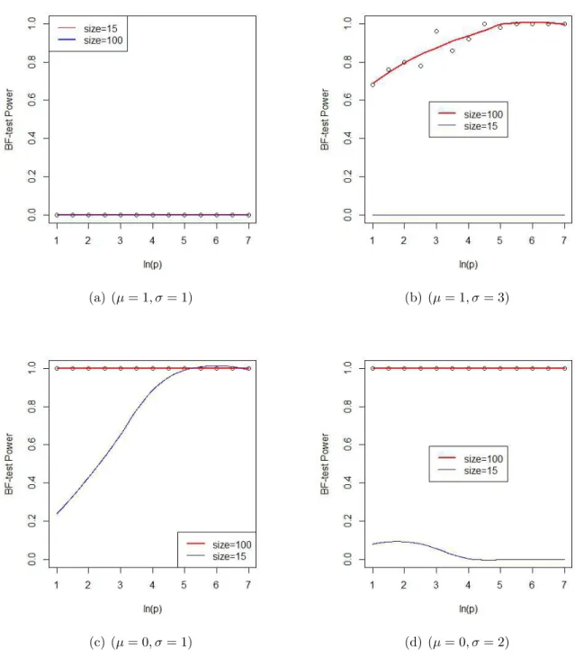
First, we will estimate the power of BF-test. We set F distributed as Np((µ, . . . , µ)

0

, σIp) whereIp stands for identity matrix. And,Gis distributed as (Exp(1), . . . , Exp(1))

0

∈Rp_{. We} consider four cases, namely (µ= 1, σ= 1),(µ= 1, σ= 3),(µ= 0, σ = 1) and(µ= 0, σ= 2). In each case, we generate n observations from each distribution to test H0 : F = G. We

choose n= 15 and 100. And, the experiment is repeated 200 times, and the proportion of times a test rejected H0 was considered as an estimate of its power. Since

TBF∗ m,n 2 r \ tr(Σ2₎ \ tr(Σ) q (m_m+₋n₁)2_{+ (}m+n n−1)2+ ( m+n √ 2mn) 2

converges to N(0,1), the null hypothesis would be rejected if test is larger than 1.96. From the plots below, we see that BF-test does not work when µ1 =µ2,σ1 =σ2. In the

(a) (µ= 1, σ= 1) (b) (µ= 1, σ= 3)

(c) (µ= 0, σ= 1) (d) (µ= 0, σ= 2)

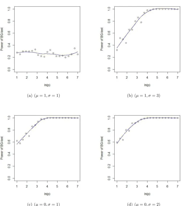
Next, we would like to estimate the power of BG-test. We would follow the same procedures. Additionally, we would like to estimate the power of BG-test in the case of HDLSS. We also consider the same four cases, namely (µ = 1, σ = 1),(µ = 1, σ = 3),(µ = 0, σ = 1) and(µ= 0, σ = 2). Since BG-test

N TBF 2ˆδ2

1(N/m+N/n)

converges to Chi-square distribution with degree freedom 1, the null hypothesis will be rejected if it is larger than 3.841.

According to the following plots 3.2, it is easy to see that BG-test also does not work when µ1 = µ2, σ1 =σ2. In other case, BG-test works very well even when sample size equals

4. Biswas and Ghosh (2014) suggested to use permutation test if sample size is small. It may not be necessary. This problem is beyond the scope of this work but it could be one of my future research topics.

3.2

Conclusions of Simulation

According to our analysis, we can say both tests are mean-variance tests. In other words, they both test H0 : EX = EY and VX = VY rather than H0 :F = G. It is because two

distributions sharing the same mean and variance may be different in many other ways. Thus, further studies are needed to propose a more sophisticated test.

(a) (µ= 1, σ= 1) (b) (µ= 1, σ= 3)

(c) (µ= 0, σ= 1) (d) (µ= 0, σ= 2)

(a) (µ= 1, σ= 1) (b) (µ= 1, σ= 3)

(c) (µ= 0, σ= 1) (d) (µ= 0, σ= 2)

REFERENCES

1. Bai and Saranadasa, H. (1996) Effect of high-dimension: by an example of a two-sample problem. Statistica Sinica, 311-329.

2. Biswas, M. and Ghosh, A. (2014). A nonparametric two-sample test applicable to high dimensional data. J. Multivariate Anal. 123, 160-171.

3. Chen, Song Xi; Qin, Ying-Li. (2010) A two-sample test for high-dimensional data with applications to gene-set testing. Ann. Statist. 38 (2010), no. 2, 808–835. doi:10.1214/09-AOS716

4. Fan, Jianqing; Fan, Yingying. (2008) High-dimensional classification using features annealed independence rules. Ann. Statist. 36 , no. 6, 2605–2637. doi:10.1214/07-AOS504. http://projecteuclid.org/euclid.aos/1231165181.

5. Friedman, J. H. and Rafsky, L. C. (1979). Multivariate generalizations of the Wald-Wolfowitz and Smirnov two-sample tests. Ann. Statist. 7, 697-717.

6. Henze, N. (1988). A multivariate two-sample test based on the number of nearest neighbor type coincidences. Ann. Statist. 16, 772-783.

7. Hall, P., Marron, J. S. and Neeman, A. (2005), Geometric representation of high dimension, low sample size data. Journal of the Royal Statistical Society: Series B (Statistical Methodology), 67: 427-444. doi: 10.1111/j.1467-9868.2005.00510.x

8. Rauf Ahmad (2014) A U-statistic approach for a high-dimensional two-sample mean testing problem under non-normality and Behrens-Fisher settingAnnals of the Institute

of Statistical Mathematics 0020-3157 66:1

9. Rauf Ahmad, M., von Rosen, D. and Singull, M. (2013), A note on mean testing for high dimensional multivariate data under non-normality. Statistica Neerlandica, 67: 81-99. doi: 10.1111/j.1467-9574.2012.00533.x

10. Serfling, R. J. (1980). Approximation theorems of mathematical statistics. New York: Wiley

11. Schucany, W. R. and Bankson, D. M. (1989), Small sample variance estimators for U-statistics. Australian Journal of Statistics, 31: 417426. doi: 10.1111/j.1467-842X.1989.tb00986.x

12. Sen, P.K. (1960). On some convergence properties of U-statistics. Cal. Statist. Assoc. Bull. 10 1-18

13. Sungkyu Jung, Arusharka Sen, J.S. Marron, Boundary behavior in High Dimension, Low Sample Size asymptotics of PCA, Journal of Multivariate Analysis, Volume 109, August 2012, Pages 190-203, ISSN 0047-259X.

14. Tao, T. (2012) Topics in Random Matrix Theory, isbn: 9780821885079, American Mathematical Soc.