Lévy processes and Lévy copulas with an application in insurance

(1)

Thesis for the degree of Master of Science

Mathematical statistics

University of Bergen, Norway

June 1, 2007

Martin Hunting

Lévy processes and Lévy copulas

(2)

(3)

Acknowledgments

I would like to express deep gratitude to my advisor, Trygve S. Nilsen, for coping with my foolhardiness and, more than once, forcing me back to the right track when I got lost. I would also like to thank Marius Fredheim for making me aware of the Danish fire insurance dataset and Karl Ove Hufthammer for helping me solve a multitude of technical problems and issues. Not least would I like to thank my father for invaluable proofreading assistance.

(4)

(5)

This thesis deals with infinitely divisible distributions and Lévy processes. Key-words: Infinitely divisible distributions, stable distributions, Levy copula, compound Poisson distribution, generalized Pareto distribution.

(6)

Notation

; the empty set w.r.t with respect to a.s. almost surely

a.e. almost everywhere with respect to the Lebesgue measure i.i.d. independent and indentically distributed

unspecified set

#A the number of elements of a setA := defined as d = equal in distribution d → convergence in distribution Dom domain Ran range

R the set of real numbers

R the extended set of real numbersRS{−∞,+∞}

t time.

T transpose

Aû _{the complement of the set}_A C the set of complex numbers

|c_| absolute value ofc or, ifc is complex, the modulus ofc ¯

z The conjugate of the complex numberz × Cartesian product

Rd thed-dimensional spaceR×R×. . .×R

| {z }

dtimes B(Rd₎ _{the Borel}_σ_{-algebra of}

Rd,

i.e. theσ-algebra generated by the open sets of_Rd m(B) the Lebesgue measure of a setB.

m(dx)is writtend x Nn

1Aj productσ-algebra of theσ-algebrasA1. . .An. Rd d-dimensional spaceR×R×. . .×R

| {z }

dtimes card cardinality

〈a,b_〉 scalar product of vectorsaandb 0 (0, 0, . . . , 0)generalized origo vector b

P Fourier transformation of the probability distributionP f+(x) max(0,f(x))

(10)

f(x)∼g(x) lim_x_→_a f(x)

g(x) =1 for some limit pointa∈R.

In this thesisawill be_∞unless otherwise specified. f(x) =O(g(x)) lim_x_→_a|f(x)|

|g(x)| <∞for some limit pointa∈R. f(x) =o(g(x)) lim_x_→_a|f(x)|

|g(x)| =0 for some limit pointa∈R. 1A(x) indicator function:

=1 ifx ∈A =0 otherwise

h∈ Rγ his a regular varying function with indexγ.

Cn Class of all functions whose partial derivatives of order_≤n all exist and are continuous.

sign(x) sign ofx, i.e.+1 ifx≥0, ₋1 ifx<0. C(f) points where f is continuous

sup supremum, the least upper bound inf infemum, the greatest lower bound lim_x_↓_ag(x) limit ofg(x), lettingx decrease towardsa lim_x_↑_ag(x) limit ofg(x), lettingx increase towards a

(11)

1

Introduction

1.1 Topics covered in the thesis

This thesis discusses Lévy processes and Lévy copulas. In connection with Lévy processes we treat some of the theory behind infinitely divisible distributions, acknowledging that the two classes are equivalent. Within the class of Lévy processes we will mostly look at stable processes and compound Poisson processes.

1.1.1 Lévy processes

Origin of Lévy processes

The theory of Lévy processes dates back to the late 1920’s, after de Finetti first

introduced the class of infinitely divisible distributions. In 1934 those distributions

were shown by Paul Lévy to have characteristic functions of the form given by the Lévy-Khintchine formula. Since then Lévy processes have become popular tools for modelling in finance, insurance and physics.

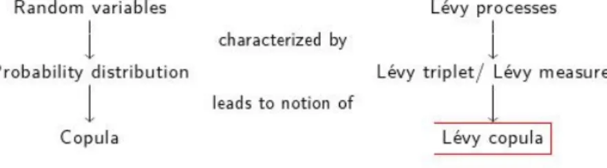
1.1.2 Lévy copulas

Copulas are functions that can be regarded as (a) functions that join or “couple” a

multidimensional distribution to its one-dimensional margins or (b) as multivariate

(12)

In Tankov (2003b) Peter Tankov introduced Lévy copulas to model the dependen-cies between components of a multidimensional spectrally positive Lévy process. Lévy copulas for more general Lévy processes are discussed in

Cont and Tankov (2004). Lévy copulas have many similarities with other copula functions, but have the domain[0,∞]d _for_d₌_{2, 3, . . . rather than}_[_{0, 1}_]d_.

1.1.3 Stable processes

In this thesis we implement an algorithm given on page 202 in Cont and Tankov (2004) for simulation of a two-dimensional Lévy process whose components are

stable processes with stable distributions. Stable distributions are characterized by:

• Having the stability property (see definition 3.3.2 on page 27).

• The fact that a distribution has a domain of attraction (defined in defini-tion 2.1.6 on page 13) if and only if it is stable.

• Having infinite variance (except for the Gaussian distribution).

• Having an indexα_∈(0,2]. Thix index will be explained in section 3.3.2 on page 27.

Stable processes are stochastic processes whose increments obey a stable

dis-tribution. For a stable process the stability property translates into the concept of

self-similarity (defined in definition 4.2.1 on page 39).

1.2 Compound Poisson processes

A favoured approach in insurance is to model a risk process as a compound Poisson

process, with positive jumps representing the insurance claims. Classical ruin theory is based on the assumption that all the claims are independent and identically distributed. The assumption of all claims being independent is dropped in Bregman and Klüppelberg (2005). Discussed there are two dependent compound Poisson

processesX_t andY_t with positive jumps and whose dependence is described by a

Clayton Lévy copula. The sumX_t+Y_t is identified as a compound Poisson process

with new Poisson intensity and claim distribution.

(13)

using the multivariate Danish fire insurance claims dataset provided by Alexander

McNeil and available from

http://www.ma.hw.ac.uk/~mcneil/data.html.

1.3 Applications of Lévy processes

1.3.1 Lévy processes in finance

As described in the introduction of Schoutens (2003), modelling financial mar-kets with stochastic processes began in 1900 with Bachelier (1900). He modelled the prices of stocks listed at the Paris Bourse as aBrownian motion. Also known

as a Wiener-process, Brownian motion is a stochastic process with independent,

stationary increments that obey a Gaussian distribution. 65 years later another, more appropriate model was suggested in Samuelson (1965), where thelogarithms of the stock prices were modelled as a Wiener process. This model is known as geometric Brownian motion. In Black and Scholes (1973) it was demonstrated how to price European options based on the geometric Brownian model. This stock-price model has been widely acclaimed and is now known as the Black-Scholes model. As

pointed out in chapter 1 in Cont and Tankov (2004) there are, however, a number

of flaws with the Black-Scholes model. Some of the most serious are the following:

• Continuity:

Brownian motion is inherently continuous, while compelling empirical evi-dence has made it clear that the trajectories of log-prices have a large number of discontinuities.

• Scale invariance:

The statistical properties of Brownian motion are the same at all time res-olutions. On page 2 in Cont and Tankov (2004), the path of the log-price of SLM1in the period 1993-1997 is compared with the path of a simulated Brownian motion. While the Brownian path looks the same over a one-month period as over three years or three months, the price behavior over this period

is clearly dominated by a large downward jump, which accounts for half of

the monthly return. On anintra-dayscale the price moves essentially through jumps, while the Brownian model retains the same continuous behavior as over long horizons. As noted on page 4 in Cont and Tankov (2004), “Assuming

that prices move in a continuous manner amounts to neglecting the abrupt

movements in which most of theriskis concentrated.” • Light tails:

(14)

The empirical distribution of returns decays slowly at infinity and very large

moves have a significant probability of occuring. As an example, six-standard

deviation market moves are commonly observed in all markets. As noted by Cont and Tankov, the Gaussian distribution, in the other hand, is a light-tailed distributiion, and in a Gaussian model a daily return of such magnitude occurs on average less than once in a million years.

Many Lévy process models allow both discontinuities and heavy tails and have

therefore been suggested by several authors as candidates for option pricing models (see chapter 4 in Cont and Tankov (2004)).

1.3.2 Applications of stable processes in physics

While stable process models remain controversial in finance (for two discussions on

the matter see section 7.3 in Cont and Tankov (2004) and section 17.7 in Uchaikin

and Zolotarev (1999)), they are routinely applied in several branches of physics.

Common textbook examples where “the basic physical mechanism inexorably leads

to a description in terms of anα-stable law with a particularα”

(Woyczy´nscki (2001)) include the following (see Woyczy´nscki (2001) ) :

Example 1.3.1: The first hitting time for the Brownian particle

Consider a Brownian particle moving inRwhose trajectoryXt,t≥0, starts at X0=0. The first time, Tb>0, it hits the barrier located at x =b>0 is a random variable that can be defined by the formula

T_b=inf

t≥0 :X_t=b .

It is shown in Woyczy´nscki (2001) thatTbobeys the Lévy distribution defined

in equation 3.20 on page 33. This Lévy distribution is a stable distribution with

indexα=1/2.

(15)

Example 1.3.2: Particles emitted from a point source

Consider a source located at the point 0,η

in theR2 plane, emitting parti-cles into the right half-space with random directions (angles),Θ, uniformly distributed on the interval [−π/2,π/2]. The particles are detected by a flat panel device represented by the vertical line x =τ at the distance τ from the source. In Woyczy´nscki (2001) the probability distribution function of the random variable representing the positionY of particles on the detecting device is shown to obey a one-dimensional Cauchy distribution, defined in equation 3.3 on page 24. Cauchy distributions of any dimension are stable distributions with indexα=1.

Example 1.3.3: Stars, uniformly distributed in space

Consider a model of the universe in which the stars with massesM1≥0,i= 1,2, . . . located at positions X_i _∈_R3,i =1,2, . . . ,interact via the Newtonian gravitational potential, exerting force

G_i =g M_iXi X_i

3 ∈R

3_, _i₌_{1, 2, . . . ,}

on a unit mass located at the origin(0,0,0). Heregis the universal gravita-tional constant. Make the assumptions that

• The locations X_i,i = 1,2, . . . form a Poisson point process in _R3 with densityρ.

• The massesM_i,i=1, 2, . . . are i.i.d. variables.

Let G_R be the total gravitational force on a unit mass located at the origin, exerted by stars located inside a ballB_R, centered at(0,0,0)and of radiusR, that is

G_R= X i:|Xi|≤R

G_i

It is then shown in Woyczy´nscki (2001) that the limitlim_R_→∞G_R obeys a three-dimensional, spherically symmetric stable distribution with index

3

2. In astrophysics this distribution is known as theHoltsmark distribution.

More examples of applications of stable distributions/stable processes are found

(16)

2

Basic definitions and results

This chapter is a collection of definitions and results, mostly taken from chapters 1 and 2 in Sato (1999) and included here to be used as a reference.

2.1 Probability measure

Definition 2.1.1: Probability space

LetΩbe a set,_F a σ-algebra of subsets inΩ, and _Pa measure on_F. The triplet(Ω,F,P)is then called ameasure space. IfP(Ω) =1 then (Ω,F,P)is called aprobability space.

Given a probability space(Ω,F,P), any setA∈ F is called anevent, andP[A] is called theprobabilityof the eventA. Theσ-algebra generated by the open sets in_Rd _{is called the} _Borel_σ_-algebra_{. A real valued function} _f₍_x₎ _on

Rd is called

measurable1 if it isB(Rd₎_{-measurable. We shall say that}_F _{is a probability measure} onRd ifF is a probability measure on(Rd,B(Rd)).

1

LetΩandΘbe two abstract spaces ,Mbe aσ-algebra onΩandN be aσ-algebra onΘ. A functionf :Ω→Θis calledmeasurableif for any setE∈ N the set_ω

(17)

Definition 2.1.2: Random variable

Let(Ω,_F,P)be a probability space. A mappingX fromΩintoRd is called an Rd-valuedrandom variable(or random variable onRd) if X isF-measurable. LetB∈ BRd

. We writeP(ω:X(ω)∈B)asP(X∈B). As a mapping ofB this is a probability measure on_B(Rd), which we denote byPX and call the distribution (or law) ofX.

In general, probability measures onB(Rd)are calleddistributionsonRd. If two

random variablesX,Y onRd (not necessarily on the same probability space) have an identical distribution, i.e.PX=PY, we writeX =d Y.

Definition 2.1.3: Weak convergence

Let F_n and F be probability measures on _Rd_{. The sequence}_{_F_n} _converges

weaklytoF if¦R

Rd f(x)Fn(dx) ©

converges toR

Rd f(x)F(dx)for every function f which is real-valued, continuous and bounded onRd.

Definition 2.1.4: Convergence in distribution

Let ¦ Xn

n≥1 ©

be a sequence of Rd-valued random variables. We say {Xn} converges in distributiontoX ifP{Xn}converges weakly toPX. We writeXn

d →X.

Definition 2.1.5: Random walk

Let{Z_n:n=1,2, . . . ,}be a sequence of independent and identically distributed Rd-valued random varibles. Let S0 =0,Sn =

Pn

j=1Zj for n=1,2, . . .. Then {S_n:n=0, 1, . . ._}is arandom walkonRd.

Definition 2.1.6: Domain of attraction

LetS_n be a random walk and F be the common distribution. ThenF is said to belong to thedomain of attraction of a probability measureR if there are constants bn > 0 and constant vectors cn such that the series {bnSn+cn} converges toRin distribution.

A random variableX on the probability space(Ω,_F,P)is said to have a propertyA

almost surely(abbreviated a.s.) if there is a measurable setΩ₀_{∈ F} with_P[Ω₀] =1

(18)

If X =c a.s., wherec is constant vector in a euclidean space, we say that the distribution ofX istrivial.

If X is a real-valued random variable and if R ΩX(ω)PX(dω) <∞, then the

integral is called theexpectationof x and is denoted by_E[X]or_EX. If in addition

X is a random variable onRd, and f(x)is a bounded measurable function onRd, then E[f(X)] = Z Rd f(x)PX(dx). Definition 2.1.7: Independence

LetXj be anRdj-valued random variable for j=1, . . . ,n. The family {X1, . . . ,Xn}isindependentif, for every setBj∈ B(Rdj), j=1, . . . ,n,

P X1∈B1, . . . ,Xn∈Bn =P X1∈B1 P X2∈B2 . . .P Xn∈Bn .

We say that X1, . . . ,Xn are independent if the family{X1, . . . ,Xn}is independent.

An infinite family of random variables is independent, if every finite subfamily of it

is independent.

Definition 2.1.8: Convolution

TheconvolutionF of two distributionsF₁and F₂onRd, denoted byF =F1∗F2, is a distribution defined by F(B):= Z Z Rd×Rd 1_B(x+y)F1(dx)F2(dy). (2.1)

2.2 Probability density

2.2.1 Probability density

It can be shown (see chapter 1 in Sato (1999)) that ifX1andX2 are independent

random variables onRd with distributionsF1and F2respectively, thenX1+X2 has

the distributionF₁_∗F₂.

Definition 2.2.1: Probability density

(19)

If a probability measure on(Rn,_B(Rn))has a density, then this density is uniquely determined up to a null-set, as stated in the following theorem:

Theorem 2.2.2

A non-negative Borel-measurable function f is the density of a probability measure on(_Rn_,_B₍

Rn))if and only if it satisfies R

Rnf(x)dx=1. In this case f entirely determines the probability measure. That is, for any other non-negative Borel measurable function f0, ifmn(f ₆= f0) =0 then f0is also a density for the same probability measure.

Conversely, a probability measure on(Rn,B(Rn₎₎_{determines its density}

(when a density exists) up to a set of Lebesgue measure zero. That is, if f and

f0are two densities for this probability, thenmn(f 6= f0) =0. A proof is found in chapter 12 in Jacod and Protter (2004). We shall sometimes denote as a random vectorX= X1, . . . ,Xd

T

, whereX∈ Rd and each Xk,k =1, . . . ,d, is a R-valued random variable. We shall say that PX, i.e. the distribution ofX, is thejoint distributionof(X1, . . . ,Xd)T. Conversely, PX1, . . . ,PXd will be referred to as themarginalprobability distributions ofPX.

Two families of random vectors _{X_t_} and _{Y_s} are said to be independent if, for any choice of t1, . . . ,tn and s1, . . . ,sm, the random vectors (Xtj)j=1,...,n and

(Y_s_k)k₌1,...,mare independent.

2_{The Lebesgue measure}_m_on₍

R,B(R)S{all subsets of nullsets})measures an interval as its length.

The Lebesgue measuremn_{is the completion of the}_{n-fold product of}_m_{with itself on}Nn j=1B(R), i.e.mn₍_A

1×...×An) =

Qn

j=1m(Aj)forAj∈ B(R).SinceRis a separable space (see proposition

1.5 in Folland (1999)) we have thatNn

j=1B(R) =B(R

(20)

Theorem 2.2.3

LetX= (Y,Z)be a random vector onR2with a density f. Then

(a) Both the componentsY andZ have densities on(R,B(R)), given by: fY(y) = Z R f(y,z)dz; fZ(z) = Z R f(y,z)dy.

(b) Y andZ are independent if and only if

f(y,z) = f_Y(y)f_Z(z) for all(y,z)_∈R2\E, whereEis anm2-null set.

This theorem can be generalized to_Rn_,_n₌_{3, 4, . . . (see chapter 12 in} Jacod and Protter (2004)).

2.3 Stochastic process

2.3.1 Stochastic process on a euclidean space

Definition 2.3.1: Stochastic process

A family _{X_t : t _≥ 0_}of probability distributions on Rd with parameter t ∈

[0,_∞), defined on a common probability space, is called astochastic process. It is written as{Xt}.

It can be shown (see chapter 1 in Sato (1999)) that, for any fixed {0≤t1<t2<tn},

P

Xt1∈B1, . . . ,Xtn∈Bn

determines a probability measure on_B((_Rd₎n₎_{. The family of probability measures}

over all choices ofnand t1, . . . ,tn is called thesystem of finite-dimensional distribu-tionsof_{Xt}.

(21)

Definition 2.3.2: Cylinder set and Kolmogorovσ-algebra

LetΩ = (_Rd₎[0,∞)_{. Let}_ω_{be the collection of all functions}_ω_{= (}_ω₍_t₎₎

t∈[0,∞)

from[0,∞)intoRd. DefineXt byXt(ω) =ω(t). A set

C ={ω:Xt1(ω)∈B1,Xt2(ω)∈B2, . . . ,Xtn(ω)∈Bn}

for 0_≤t₁<_{· · ·}<t_nandB₁, . . . ,B_n_{∈ B}(Rd)is called acylinder set.

Let_F be theσ-algebra generated by the cylinder sets. Then_F is called the

Kolmogorovσ-algebra.

The following theorem by Kolmogorov ensures that a suitable “consistent” system of finite-dimensional distributions will define a stochastic process.

Theorem 2.3.3: Kolmogorov’s extension theorem

Suppose that, for any choice ofnand 0_≤t1<· · ·<tn, a distributionFt1,...,tn

is given. Suppose further that, ifB1, . . . ,Bn∈ B(Rd)andBk=Rd, then Ft1,...,tn B1×

..._×_B n

=Ft1,...,tk−1,tk+1,...tn(B1× · · · ×Bk−1×Bk+1· · · ×Bn).

Then there exists a unique probability measurePonF that has ¦

Ft1,...,tn

©

as its system of finite-dimensional distributions.

The theorem is stated on page 4 in Sato (1999). A proof can be found on page 489 in Billingsley (1986).

A stochastic process{Y_t : t ≥0}on the probability space(Ω,F,P) is called a modificationof the stochastic process_{X_t:t_≥0_}on the same probability space, if P(Xt=Yt) =1 fort∈[0,∞).

Two stochastic processes_{Xt}and{Yt}areidentical in law, written as

{X_t}=d _{Y_t_},

if the systems of their finite-dimensional distributions are identical. Considered as a function oft,X(t,ω)is called asample function, orsample path, of{Xt}.

2.3.2 Càdlàg processes

When we get to chapter 4 we shall see that stochastic continuity and the càdlàg property are two of the defining properties of a Lévy process. In this section we

(22)

define these concepts and introduce a measure for the discontinuities (jumps) of càdlàg processes (stochastic processes with the càdlàg property).

Definition 2.3.4: Stochastic continuity

A stochastic process_{X_t:t_≥0_}on a probability space(Rd,_F,P)is said to be

stochastically continuousif, for every t≥0 and everyε >0, lim

s→tP(|Xs−Xt| ≥ε) =0. (2.2) ‘

Definition 2.3.5: Càdlàg

LetX_t be a stochastic process on the probability space(Rd,_F,P). We say that X_t has thecàdlàg property if there existsΩ0_{∈ F} withP(Ω0) =1 such that, for

everyω∈Ω0,X_t(ω)is right-continuous in t≥0 and has left limits in t>0.

Definition 2.3.6: Jump times of a càdlàg process

LetXbe a stochastic process with the càdlàg, property. For a given timet we

shall denote the left limitlim_s_↑_tX_s, byX_t₋and the differenceX_t₋X_t₋by∆X_t. For a given time interval(a,b)we shall call the set

t_∈(a,b):∆X_t 6=0 the jump timesof_{X_t:t≥0_}in(a,b).

For a càdlàg process_{X_t: t_≥0_}onRd we introduce a measureJX. For every Borel measurable setA∈Rd, JX([t1,t2]×A)counts the number of jump times of X_t betweent1 andt2with jump sizes inA.

2.4 Characteristic functions

The principal analytical tool in this thesis is the Fourier transform, which in the statistical community is known under the namecharacteristic function.

Definition 2.4.1: Characteristic function

Thecharacteristic functionof a probability measureF onRd is defined as

b F(u):=

Z

Rd

(23)

Definition 2.4.2

The characteristic function of the distribution_PX of a random variableX on Rd is defined as b PX(u):= Z Rd ei〈u,x〉PX(dx) =E ei〈u,X〉. (2.3)

It follows immediately from definition 2.4.2 that ifX is a random vector on_Rd_,_a is a real constant andb_∈Rd is a constant vector, then

b

PaX+b(u) =ei〈u,b〉PbX(au). (2.4)

Theorem 2.4.3

The following theorem sums up some of the most important properties of characteristic functions.

Let F andF1,F2, . . . ,Fn be distributions onRd.

(i) (Bochner’s theorem) ThenFb(0) =1 and|Fb(u)| ≤1. AlsoFb(u)is uniformly continuous nonnegative-definite in the sense that, for eachn=1, 2, . . . ,

n X j=1 n X k=1 b F(u_j₋u_k)z_j¯z_k≥0 for allu₁, . . .u_n_∈_Rd,z1, . . .zn∈C. Conversely, if a complex-valued functionϕ(u) onRd withϕ(0) =1 is

continuous atu=0and is nonnegative-definite, thenϕ(u)is the

charac-teristic function of a distribution on_Rd_.

(ii) IfcF₁(u) =cF2(u)for allu∈Rd thenF₁=F₂.

(iii) IfF =F1∗F2, then Fb(u) =cF1(u)cF2(u)for allu∈Rd. IfX1 andX2 are independent random vectors onRd then

b

PX1+X2(u) =bPX1(u)PXb 2(u) for allu∈R

(24)

(iv) LetX= (X_j, . . . ,X_n)be an_Rnd_{-valued random vector, where}

X₁, . . . ,X_nareRd-valued random vectors. ThenX1, . . . ,Xnare independent if and only if

b

PX(u) =bPX1(u1). . .PbXn(un) for allu= (u1, . . . ,un),

whereu_j_∈_Rd _for _j₌_{1, . . . ,}_n.

(v) Letnbe a positive integer. IfF has a finite absolute moment of ordern, that is ifR_|x_|n_F₍_dx₎_<_∞_{, then}

b

F(u)is a function of classCn (continuous n-th derivative) and, for any nonnegative integersn₁,n₂, . . .n_d satisfying

n1+· · ·+nd ≤n, Z xn1 1 . . .x nd d F(dx) = ₁ i ∂ ∂u1 n1 ... ₁ i ∂ ∂ud nd b F(u) u=0 .

(vi) Letnbe a positive even integer. IfFb(u)is of classCn in a neighborhood of the origin, thenF has finite absolute moment of ordern.

(vii) (Inversion formula) Let −∞ < a_j < b_j < ∞ for j = 1, . . . ,d and B = [a1,b1]×...×[ad,bd]. IfBis anF-continuity set,3then

F(B) = lim c→∞(2π) −d Z [−c,c]d b F(u) Z B e−i〈u,x〉dxdu (viii) If R bF

du < ∞, then F is absolutely continuous 4with respect to the Lebesgue measure and has a bounded continuous density f(x), where

f(x) = (2π)−d Z

Rd

e−i〈u,x〉Fb(u)du.

Proof: On page 10 in Sato (1999) there is a reference to where proofs can

be found.

3_{We define the boundary of a set}_B_∈

Rdas the difference between the smallest closed set inRd

containingBand the biggest open set inRdcontained inB. We say thatBis aF-continuityset if

the boundary ofBhasF-measure 0.

(25)

WhenF is a distribution on[0,∞), theLaplacetransform ofF is defined by LF(u) = Z [0,∞) e−uxF(dx) foru≥0. (2.6) Proposition 2.4.4

Let F,F₁, andF₂be distributions on[0,∞). (i) If L_F₁(u) =L_F₂(u)for allu≥0, thenF1=F2. (ii) IfF =F₁_∗F₂, then L_F(u) =L_F₁(u)L_F₂(u).

Proof: For a proof see proposition 2.6 in Sato (1999).

Lemma 2.4.5

Suppose thatφ(u)is a continuous function fromRd intoCsuch thatφ(0) =1 andφ(u)6=0 for anyu_∈_Rd_{. Then there is a unique continuous function} _f₍_u₎ from Rd into C such that f(0) =0 and ef(u) =φ(u). Also for any positive

integernthere is a unique continuous functiongn(u)fromRd intoCsuch that gn(0) =1 and

gn(u)n=φ(u). f and gnhave the relation gn(u) =ef(u)/n. Proof: For a proof see lemma 7.6 in Sato (1999).

We write f(u) =logφ(u)and gn(u) = [φ(u)]1/n. We call f and gn the distin-guished logarithmand thedistinguished nth rootofφ, respectively. For all

r_≥0,[φ(u)]r=er f(u). We caller f(u)thedistinguished rth powerofφ. IfFbu r

is

the characteristic function of a probability measure, then we denote this probability measure byFr.

(26)

3

Infinitely divisible distributions

3.1 Definitions and basic examples

This chapter discusses a class of probability distributions known asinfinitely divisible distributions. We begin by presenting some general results about all distributions in

this class before we go on to discuss a sub-class known asα-stable distributions.

Definition 3.1.1

A probability measure F on_B(Rd)isinfinitely divisibleif for any integern≥2 there existni.i.d. non-trivial random variablesY(₁n), . . .Y(n)

n such that Y(₁n)+· · ·+Y(_nn)has the distribution F.

Let us now consider an alternative definition of infinitely divisible distributions.

The following is shown in Cont and Tankov (2004) and uses the fact that the distribution of sums of i.i.d. variables is given by the convolution of the distribution of the summands. For any n≥ 2 let Fn be the distribution of each of the above Y(₁1), . . . ,Y(_nn). Then then-th convolution ofF_n, namelyF_n∗..._∗_F

n ntimes, is equal toF.

Therefore an infinitely divisible distribution can also be defined as a distribution

F for which, for anyn≥2, there exists a probability measureF_n onBRd

such that F is equal to then-th convolution ofF_nwith itself:

(27)

Example 3.1.2

Ford≥2 letF be the nondegenerate1Gaussian distribution onRd with mean vectorµand covariance matrixQ, whereQis a symmetric non-negative definite, invertible matrix . Then F has the probability density

(2π)−d_(det_Q)−1/2_e−〈x−µ,Q−1₍_x₋_µ₎_〉_/₂

(3.1) for allx_∈Rd. It can then be shown (see chapter 2 in Sato (1999)) that

b F(u) =exp −1 2〈u,Qu〉+i〈u,µ〉 , u_∈Rd. (3.2)

By choosingF_n to be the Gaussian distribution onRd with mean vector 1_nµ and covariance matrix 1_nQ, we trivially get that the Gaussian distribution is infinitely divisible.

The Gaussian distribution owes much of its importance in statistics to its large domain of attraction, formalized in the Central Limit Theorem below.

Theorem 3.1.3: Central Limit Theorem

LetS_n be a random walk onRd. Here each i.i.d. step X_j,=X(_j1), . . . ,X(_jd)T has

(a) a finite mean vectorµand

(b) a finite covariance matrixQ=qk,l

withk,l=1, . . . ,d. Hereqk,l =Cov

X(_jk),X(_jl), whereX(_jk)andX(_jl)are thek-th andl-th com-ponents of theRd-valued random variableXj. Then

_S n−nµ p n d →Z,

where Z is a d-dimensional Gaussian-distributed random vector with mean vector0and covariance matrixQ.

Proof: A proof can be found on page 238 in Breiman (1968).

1_{A Gaussian distribution is called}_degenerate_{if the covariance matrix}_Q_{is singular, i.e.}

(28)

Example 3.1.4

LetF be thed-dimensional Cauchy distribution with parameters γ∈Rd andc>0. That is, let F have the density

Γ((d+1)/2)π−(d+1)/2(|x₋γ|2) +c2−(d+1)/2 forx_∈Rd. (3.3) It can be shown (see page 11 in Sato (1999)) that the Cauchy distribution has the characteristic function

b

F(u) =e−c|u|+i〈γ,u〉. (3.4) LetF_n be thed-dimensional Cauchy distribution with parameters

1 nγ ∈ R

d _and 1

nc > 0. We then see that

c

Fn(u)n = Fb(u), so the Cauchy distribution is infinitely divisible.

Example 3.1.5

A trivial example of a function that is not infinitely divisible is the uniform distribution on(a,b), whose characteristic function is

eiub−eiua

iu . (3.5)

3.2 The Lévy-Khintchine representation

3.2.1 The formula

The most useful analytical tool for studying infinitely divisible distributions is the characteristic function. This is in large part due to a theorem that says that the characteristic function of every infinitely divisible distribution is of a closed form specified by the Lévy-Khintchine representation.

Theorem 3.2.1

LetD={x:_|x_{| ≤}1_}.

IfF is an infinitely divisible distribution onRd, then there existQ,ν andγ such that

(29)

b F(u) =exp

[

−1 2〈u,Qu〉+i〈γ,u〉 + Z Rd ei〈u,x〉₋1₋i_〈u,x_〉1D(x)ν(dx)

]

. (3.6) HereQis a symmetric nonnegative-definited×dmatrix,ν is

on_Rd_{\ {}₀_}_withR

min(1,_|x_|2)ν(dx)<_∞andγa vector in_Rd_. The three parametersQ,ν andγare unique.

Proof: A proof of the one-dimensional case is found on page 192-194 in Breiman (1968).

The triplet(Q,ν,γ)is called thegenerating tripletof the infinitely divisible ran-dom variableX.

Ifν(B) =0 for any Borel setB andγ=0, then the Lévy-Khintchine representa-tion gives the characteristic funcrepresenta-tion of a centeredd-variate

Gaussian distribution with covariance matrixQ (or the variance Q ifd =1). We shall therefore refer to the parameterQas theGaussian coefficient. We shall refer to ν as theLévy measure.

3.2.2 Drift and center

As shown in Remark 8.4 in Sato (1999) , ifR

|x|≤1|x|ν(dx)<∞, then equation 3.6 can be written as b F(u) =exp −1 2〈u,Qu〉+i〈γ0,u〉+ Z Rd ei〈u,x〉−1ν(dx) . where γ0∈Rd is defined as γ0:=γ− Z Rd x1_|x|≤1ν(dx). (3.7) For reasons that will become clear in section 4.2.2 we shall then callγ₀thedrift ofP.

Similarly, ifR

(30)

then equation 3.6 on the preceding page can be written as b F(u) =exp −1 2〈u,Qu〉+i〈γ1,u〉+ Z Rd ei〈u,x〉₋1₋i_〈u,x_〉ν(dx) , (3.8) whereγ₁_∈_Rd _{is defined as} γ1:=γ+ Z Rd x1_|_x_|_>1ν(dx). (3.9) Let F_j, with j∈1, . . . ,d, denote the marginal distributions on_RofF.

It can then be shown (see Example 25.12 in Sato (1999)) that the condition R

|x|>1 |x| ν(dx) < ∞is equivalent to R

Rd|x|F(dx) <∞, and that for each j ∈

1, . . . ,dthe componentγ(₁j)ofγ₁is the expectation value ofFj. We shall callγ1the

centerofF.

3.3 Stable distributions

In this section we will look at a family of infinitely divisible distributions known asstable distributions, defined in chapter 2 in Samorodnitsky and Taqqu (1994) as follows:

3.3.1 Stability and infinite divisibility

Definition 3.3.1

A random vectorXon_Rd _{is said to have a}_stable_{distribution if, for every}_a_>₀ and everyb>0, there exist a positive number cand a vectord∈Rd such that aX(1)+bX(2)=d cX+d, (3.10) whereX(1)andX(2)are any i.i.d. random vectors independent ofX, but with the same distribution asX.

If, for anya>0 and any b>0, equation 3.10 holds withd=0, thenXis said to bestrictlystable.

(31)

Xis calledsymmetric stableif it is stable and

F{X_∈A}=F{−X_∈A} (3.11) for any Borel setAofRd, where F is the distribution ofX.

An alternative and equivalent definition of a stable distribution is the following

(see page 69 in Sato (1999)):

Definition 3.3.2

Let F be an infinitely divisible probability measure on_B_Rd

. F is called stableif, for anya>0, there exist b>0 andc_∈Rd such that

[Fb(u)]a=Fb(bu)ei〈

c,u〉_. _(3.12)

It is calledstrictly stableif, for anya>0, there exists b>0 such that

[bF(u)]a=Fb(bu). (3.13) F is called symmetric stable if F is stable, and for any Borel set B of Rd, F_{−x:x _∈B_}=F_{x:x _∈B_}.

Stable distributions are also characterized by the fact that a distribution posseses

a domain of attraction (see definition 2.1.6 on page 13) if and only if it is stable (see theorem 1 XVII.5 in Feller (1971).

3.3.2 Index of stability

As stated in the theorem below, any linear combination of the components of a stable distribution is stable.

Theorem 3.3.3

LetX= (X1, . . . ,Xn)T be a non-trivial and stable (respectively, strictly stable, symmetric stable) random vector in_Rd_{. Then there is a constant}_α_∈₍_0,₂_]_such that, in equation 3.10 on the preceding page,

c= (aα+bα)1/α. Moreover, any linear combination of the components ofXof the typePd_k₌₁bkXk is a stable (respectively, strictly stable, symmetric stable) random variable. A proof can be found on page 58 in

Samorodnitsky and Taqqu (1994).

As a corollary of theorem 1 in chapter VI.I in Feller (1971) and theorem 3.3.3 above we have the following:

(32)

Corollary 3.3.4

LetXbe a non-trivial random vector andX(1),X(2), . . . ,X(n)be any i.i.d random vectors independent ofX, but with the same distribution asX.

ThenXis stable if and only if there exists anα_∈(0,2]such that, for any n≥2, there exists a displacement vectord_nsuch that

X(1)+X(2)+_{· · ·}+X(n)=d n1/αX+d_n. (3.14) The indexαis called theindex of stability, and a stable distribution with index of stabilityαis called anα-stabledistribution.

Similarly, theorem 13.11 and theorem 13.15 in Sato (1999) give that in equa-tion 3.12 on the previous page

b=aα1_. _(3.15)

Theαin equation 3.15 is the same as in equation 3.14.

Example 3.3.5: Gaussian distribution (revisited)

It follows from equation 3.2 on page 23 and equation 2.4 on page 19 that if Xis ad-dimensional centered and Gaussian distributed random vector ( mean vector 0) with covariance matrix Q, and if X(1), . . . ,X(n) are n independent copies ofX(na positive integer), then

b PX(1)₊_···₊_X(n)(u) =E ei〈u,X(1)+···+X(n)〉 = E ei〈u,X〉n = exp1 2〈u,Qu〉 n =exp1 2 〈n1/2u,n1/2Qu〉 =bPX(n1/2u) =bP_n1/2_X(u).

Since two distributions are equal when their characteristic functions are equal we have that

(33)

Therefore a centered Gaussian distribution is a strictly stable distribution with index 2.

Now let us consider the general Gaussian distribution. Let Y(k) := X(k)+ µ where µ _∈_Rd_{. From the above the general Gaussian distribution can be} expressed as follows:

Y(1)+· · ·+Y(n)=d X(1)+· · ·+X(n)+nµ=d n1/2X+nµ.

Therefore a general Gaussian distribution with meanµis stable with index

α=2 and displacement vectord_n=nµ.

The following argument shows that all non-trivial stable distributions with finite covariace matrices are Gaussian: Suppose thatXis a stable random vector with a finite covariance matrixV 6=0. From the above (a) the sum ofn≥2 independent copies ofXhas a finite covariance matrixnV 6=0and

(b)n1/αXhas the finite covariance matrixn2/αV ₆=0. Because of the stability

property ofXwe must havenV =n2/αV, which impliesα=2. It follows that a

non-deterministic stable random vector with finite covariance must have index

2. Because of the central limit theorem (theorem 3.1.3 on page 23)X must be Gaussian distributed.Thus the Gaussian distribution is the only non-trivial

stable distribution with finite covariance matrix. On page 77 in Sato (1999) it

is also proven that if a stable distribution has index 2 then it is Gaussian.

Example 3.3.6: Cauchy distribution (revisited)

From equation 3.4 on page 24 it follows that if Xis a Cauchy distributed random vector andX(1), . . . ,X(n)_{are independent copies of}_{X, then}

b PX(1)₊_···₊_X(n)(u) =E ei〈u,X(1)+···+X(n)〉 = E ei〈u,X〉n = e−c|u|+i〈γ,u〉n =e−c|nu|+i〈γ,nu〉 =bP_X(nu).

Combined with equation 2.4 on page 19 and item ii on page 19 we have that

(34)

Thus the Cauchy distribution is a stable distribution with index 1.

In the remaining discussion of stable distributions we shall assume that the random variables involved are all non-trivial.

3.3.3 Stable linear combinations, unstable joint distribution

The converse of theorem 3.3.3 on page 27 is not true. There exist random vectors

that are not stable although any linear combination of their components is stable. An example of such an non-stable random vector is given in chapter 2 in Samorodnitsky and Taqqu (1994).

If some additional conditions are satisfied, however, stability of a random vector

can be inferred.

Theorem 3.3.7: Conditions for joint stability

(a) If all linear combinationsY =Pd_k₌₁bkX(k)have strictly stable distributions, thenXis a strictly stable random vector in_Rd_.

(b) If all linear combinations are symmetric stable, thenXis a symmetric stable random vector inRd.

(c) If all linear combinations are stable with index of stability greater than or

equal to one, thenXis a stable random vector in_Rd_.

(d) If all linear combinations are stable andXis infinitely divisible thenXis stable.

Proof: Proofs of the assertions above except the last one can be found on page 59 in Samorodnitsky and Taqqu (1994). A reference to a proof of item d is listed on page 65 in Samorodnitsky and Taqqu (1994).

(35)

3.4 Characteristic function of a stable distribution

In this section we state some results for the characteristic function of anα-stable random vector.

In addition to the Lévy-Khintchine -representation, another popular

representa-tion of the characteristic funcrepresenta-tion of anα-stable distribution is by means of a finite

measure on a unit sphereSd∈Rd. This representation stems from the following theorem:

Theorem 3.4.1: Characteristic function of a stable distribution

F is anα-stable distribution onRd with 0< α <2 if and only if there exists a finite non-zero measureΓon_Rd _{and a vector}_τ_in

Rd such that (i) Ifα6=1 b F(u) =exp  − Z Sd |〈u,s_〉|α 1₋itanπα 2 sign(〈u,s〉) Γ(ds) +i〈u,τ〉  . (3.16) IfXisα-stable withα6=1 thenXis strictlyα-stable if and only ifτ=0. (ii) Ifα=1 then b F(u) =exp  − Z Sd |〈u,s〉| 1+i2 π(〈u,s〉)ln|〈u,s〉| Γ(ds) +i〈u,τ〉  . (3.17)

IfF is 1-stable then F is strictly 1-stable if and only if Z

Sd

s_kΓ(ds) =0 fork=1, 2, . . . ,d.

For both cases the following hold: (a) The measureΓand the vectorτabove are unique. (b)F is a symmetricα-stable distribution onRd if and only ifΓis a symmetric measure, i.e.Γ(B) = Γ(−B)for allB∈ B(Rd), andτ=0.

(36)

Proof: This is a combination of theorem 2.3.1,theorem 2.4.1 and 2.4.3 in Samorodnitsky and Taqqu (1994).

3.4.1 Simplified Lévy measure

Theorem 3.4.2

A probability measure F on Rd isα-stable with 0 < α <2 if and only if it is infinitely divisible with generating triplet(0,ν,γ) and there exists a finite measureλonS_d, a unit sphere ofRd, such that

ν(B) = Z Sd λ(dξ) Z ∞ 0 1B(rξ) dr r1+α. (3.18)

Further, ifα=1, then F is strictly 1-stable if and only if either F is 1-stable, ν6=0, and the measureλin equation 3.18 satisfies

Z

Sd

ξλdξ=0, orQ=0,ν=0, andγ6=0.

Proof: For a proof of the first assertion in this theorem see page 78 in Sato (1999). For a proof of the second (involvingα=1) see Remark 14.6 and

theorem 14.7 in Sato (1999).

In the one-dimensional caseSd={−1,1}, so equation 3.18 reduces to (see page 80 in Sato (1999))

ν(x) = A

xα+11x>0+ B

|x|α+11x<0, (3.19) whereAandBare positive constants.

3.4.2 Probability densities of stable distributions

Before going on to Lévy processes in the next chapter, we remark the following.

Ex-cept for the Gaussian distribution and the Cauchy distribution there is unfortunately only one known case where the probability density of a stable distribution can be expressed analytically. That case is the Lévy distributionS1

2

0, 1,µ

(see chapter 3 in Cont and Tankov (2004)) which has index 1₂ and the following probability

(37)

σ 2π 1/2 ₁ (x−µ)3/2exp −₂_(xσ −µ) 1_x_>µ. (3.20) Furthermore it can be shown that the Lévy distribution above has the Lévy measureν(x) = ₂pσ_π 1

(38)

4

Lévy processes

4.1 Basic properties and one example

Definition 4.1.1

A stochastic process_{X_t,t≥0_}on the probability space(Rd,_F,P) is a Lévy process if the following conditions are satisfied:

• For any choice ofn≥1 and 0_≤t_o≤t1· · · ≤tn the random vectorsX_t₀,X_t₁₋X_t₀, . . . ,X_t

n−Xtn−1 are independent

(independent increments property).

• X₀=0 a.s.

• The distribution ofX_s₊_t−X_sdoes not depend ons(stationary increments property)

(39)

• There existsΩ₀_{∈ F} with_P(Ω₀) =1 such that, for everyω_∈Ω₀,X_t(ω) is right-continuous in t_≥0 and has left limits in

t>0. (The “càdlàg” property.)

In the following theσ-algebra_F will be onB(Rd₎_{(the Borel sets in} Rd).

4.1.1 Lévy processes are infinitely divisible

Looking at an arbitrary Lévy process (X,P)and using the decomposition X1=X1/n+ (X2/n−X1/n)· · ·+ (Xn/n−Xn−1/n),

we see that the distributionP(X₁_∈)is infinitely divisible. A similar decomposition

can be done (see Bertoin (1996)) to show that, for any rational numbert ≥0, the probability measureP(X_t_∈)is infinitely divisible as well, and

b PXt(u) =E ei〈u,Xt〉= E ei〈u,X1〉t=bPX1(u) t , whereu_∈Rd. (4.1)

4.1.2 Infinitely divisible distributions viewed as Lévy processes

Example 4.1.2

Poisson process:

Letc>0. The Poisson distribution with mean cis defined by the probability

measure F({k}) = c k k!e −c _for_k ∈0, 1, 2, . . . ,

where F(B) =0 for anyBnot containing a non-negative integer. We have that

b

A stochastic process {X_t : t ≥ 0} onR is aPoisson process if it is a Lévy process and, for t>0,X_thas Poisson distribution with meanc t.

The sample paths of a Poisson process are characterized by the following theorem (see page 308 in Breiman (1968)).

(40)

Theorem 4.1.4

A stochastic process_{Xt:t≥0}with stationary, independent increments

has a modification with all sample paths constant except for upward jumps

of length one if and only if there is a parameter c_≥0 such thatPXb

t(u) =

From equation 4.1 on the preceding page and theorem 2.4.3 on page 19 we

have that such a stochastic process is a Poisson process.

In the proof of theorem 4.1.4 Breiman also shows that the waiting times between the jumps of a Poisson process are exponentially distributed with parameterc, i.e. are gamma distributed with parameters 1 andc.

Definition 4.1.5

A distributionF onRd iscompound Poissonif, for somec>0 and for some distributionρon_Rd _with_ρ{₀_}₌_0,

b

F(u) =exp

c(ρ(_b u)₋1) for allu_∈Rd.

Hereρ(b u)is the characteristic function ofρ.

Letc>0 and letρbe a distribution onRd withρ({0})=0. A stochastic process_{X_t:t≥0_}on_Rd _{is a}_{compound Poisson process}_{associated with}_c andρif it is a Lévy processes and, fort>0, the characteristic function of the law ofX_t has the following form:

b

PXt(u) =exp t c(ρb(u)−1)

for allu∈Rd. (4.2)

Herecandρare uniquely determined byX_t.

(41)

Theorem 4.1.7

Let _{Nt : t ≥ 0} be a Poisson process with parameter c > 0 and let

S_n:n∈0, 1, . . . , be a random walk on _Rd _{with a common}

probabil-ity space(Ω,_F,P). Assume that

N_t and that

S_n are independent and

P[S₁=0] =0. Define

X_t(ω) =S_N

t(ω)(ω).

Then_{X_t:t_≥0_}is a compound Poisson process satisfying equation 4.2 on the preceding page, withρbeing the distribution ofS₁.

Proof: A proof can be found on page 18 in Sato (1999)

Compound Poisson distributions play a special role in the theory of infinitely

divisible distributions, in part because of the following theorem:

Theorem 4.1.8

Every infinitely divisible distribution is the limit of a sequence of compound Poisson distributions.

Proof: For a proof see corollary 8.8 in Sato (1999).

Because of theorem 4.1.8 it is always possible to approach a given infinitely

divisible law using a sequence of compound Poisson distributions. Using this idea it

is shown in Bertoin (1996) that every infinitely divisible distribution can be viewed

as the distribution of a Lévy process evaluated att =1. This result, combined with the above decomposition of Lévy processes, implies that the classes of infinitely divisible distributions and Lévy processes are equivalent.

Theorem 4.1.9: Infinitely divisible distributions as Lévy processes

Let there be given the following:γ∈Rd, a positive nonnegative-definite d-dimensional matrixQ, and a measureν onRd\ {0}such that

R

min(1,_|x_|2)ν(dx)<_∞. For everyu_∈Rd let

φ(u) =i〈γ,u_{〉 −}1 2〈u,Qu〉+ Z Rd ei〈u,x〉−1₋i〈u,x_〉1_|_x_|≤₁ν(dx) (4.3) and letP(u) =b etφ(u).

Then there exists a a unique probability measurePonRd under which the stochastic processX_t is a Lévy process with characteristic functionbP(u). For a proof see page 13 in Bertoin (1996).

(42)

The functionφ(u)is called thecharacteristic exponentofX_t.

In the context of Lévy processes we have (see chapter 3 in Cont and Tankov (2004)) that, for a measurable setA∈Rd, the Lévy measureν(A)can be interpreted as the expected number, per unit time, of jumps whose size belongs to the setA. I.e.,

ν(A) =E#t∈[0, 1]:∆Xt ∈A .

4.1.3 Vector space property

We refer to the following result from page 65 in Sato (1999). It shows that a linear

transformation of a Lévy process is again a Lévy process.

Proposition 4.1.10

LetX_t be a Lévy process onRd with generating triplet(Q,ν,γ)and letU be ann×d matrix. ThenY_t=UX_t is a Lévy process on_Rd_{. Its generating triplet}

QY,νY,γY is given as follows: QY=UQUT (4.4) νY= [νU−1]_Rd_\{₀_} (4.5) γY=Uγ+ Z Uy 1_E(Uy)₋1D(y) ν(dx), (4.6) whereνU−1(B) =ν({x:Ux_∈B}), for anyB∈ B(Rd),

.

4.2 Subclasses of Lévy processes

In this section we will take a closer look at stable Lévy processes and Lévy processes of finite variation.

4.2.1 Stable processes

We shall say that a Lévy process X_t is a stable, strictly stable or symmetric stable process if the distribution ofX_t at t =1 is respectively stable, strictly stable or symmetric stable.

IfXis a symmetric stable process it follows from equation 3.11 on page 27 that

(43)

Definition 4.2.1

Let_{X_t:t≥0_}be a stochastic process onRd. It is calledself-similarif , for any a>0, there exists ab>0 such that

{X_at}=d _{bX_t}. (4.7)

X_t is called broad-sense similar if for any a > 0 there exist b > 0 and a functionc(t)from[0,∞)toRd such that

X_at=d bX_t+c(t). (4.8)

The following reasoning shows that this self-similar property is shared by all strictly stable stochastic processes.

From definition 3.3.2 on page 27 and equation 3.15 on page 28 it follows that if

X_t is a strictlyα-stable process, then for any constanta>0, b PXt(u) a =Pb_X t(a 1/α_u₎_. _(4.9)

From equation 4.9 , equation 4.1 on page 35 and equation 2.4 on page 19 it follows that for anyk,t>0

b Pk−1/α_X kt(u) =bP_X kt(k −1/α_u₎ = b PXt(k −1/α_u₎k =bP_X t(k −1/α_uk1/α₎ =bPXt(u).

From the uniqueness item ii on page 19 it follows thatX_kt has the same law as

X_t, i.e.X_t is a self-similar stochastic process.

A similar calculation with a stable process using equation 2.4 on page 19 shows

that stable processes possess the broad-sense similar property. The converse is also

true, as stated in the following proposition.

Proposition 4.2.2

A Lévy-process onRd is self-similar or broad-sense similar if it is respectively strictly stable or stable.

(44)

Proof: A proof is given on page 71 in Sato (1999).

The following theorem further elucidates the relation between stable and strictly

stable processes:

Theorem 4.2.3

(i) If{X_t : t ≥0}isα-stable with 0< α <1 or 1< α≤2, then for some k_∈Rd,{Xt−tk}is strictlyα-stable.

(ii) If_{X_t:t≥0_}is 1-stable, then for any choice of a functionk(t),_{X_t₋k(t)} is not strictly 1-stable.

Proof: A proof can be found on page 82 in Sato (1999).

Due to theorem theorem 4.2.3 we shall henceforth r