Developing Forecast Techniques for Lightning Cessation Using Radar, NLDN, and LMA Analyses

(1)

DEVELOPING FORECAST TECHNIQUES FOR LIGHTNING CESSATION USING RADAR, NLDN, AND LMA ANALYSES

A Thesis by

AMANDA MARIE SINK

Submitted to the Office of Graduate and Professional Studies of Texas A&M University

in partial fulfillment of the requirements for the degree of MASTER OF SCIENCE

Chair of Committee, Richard E. Orville Committee Members, Courtney Schumacher

Brendan E. Roark Head of Department, Ping Yang

August 2016

Major Subject: Atmospheric Sciences

(2)

ABSTRACT

Dual-polarized radar data are used to develop forecast techniques for total light-ning cessation for the Houston, Texas region. A total of 42 isolated thunderstorms observed in the summer months of June, July and August of 2013 through 2015 were analyzed.

In-cloud (IC) lightning data were obtained from the Houston Lightning Mapping Array (LMA), and cloud-to-ground (CG) lightning data were obtained from the Na-tional Lightning Detection Network (NLDN). Archived radar data from the Houston Next Generation Radar (NEXRAD) radar were obtained from the National Climatic Data Center and converted to constant altitude plan projection indicator (CAPPI) format to examine at the -10, -15, and -20◦C levels. NEXRAD radar products of reflectivity and differential reflectivity were used to optimize a radar-based forecast technique for the cessation of lightning, and correlation coefficient was used to de-termine the quality of data.

Results show that the best forecast technique for the cessation of total lightning (IC and CG lightning) was the height of the 30 dBZ reflectivity value decreasing be-low the -15◦C level. This technique produced a Critical Success Index (CSI) of 82%. Results also show that the best forecast technique for the cessation of CG lightning was the 35 dBZ height decreasing below the -10◦C level, which produced a CSI of 89%.

Four differential reflectivity thresholds of -0.5, 0.5, 1, and 1.5 dB were observed in an area of 30 dBZ or greater to determine the presence of graupel and supercooled water droplets that cause charge separation and lightning within a thunderstorm. Results show that no large percentage of these thresholds decreased at a time

(3)

be-fore or after the cessation of lightning. Therebe-fore it is concluded that differential reflectivity did not aid in forecasting the cessation of lightning.

(4)

NOMENCLATURE

CAPPI Constant Altitude Plan Projection Indicator

CG Cloud-to-Ground

CRP Corpus Christi

CSI Critical Success Index

FWD Forth Worth

HCA Hydrometeor Classification Algorithm

IC In-Cloud

LCH Lake Charles

LF Low Frequency

LMA Lightning Mapping Array

NIC Non-Inductive Graupel-Ice Collison NLDN National Lightning Detection Network NWS National Weather Service

NEXRAD Next Generation Radar PPI Plan Position Indicator POD Probability of Detection POFA Probability of False Alarm

SCIT Storm Cell Identification and Tracking TOA Time of Arrival

VCP Volume Coverage Pattern VHF Very High Frequency VLF Very Low Frequency

(5)

4. CONCLUSIONS . . . 47

4.1 Conclusions . . . 47

4.2 Future Work . . . 50

(7)

LIST OF FIGURES

FIGURE Page

1.1 Tripole structure in a thunderstorm with a.) in-cloud lightning b.) cloud-to-ground lightning (Krehbiel 1986) . . . 3 2.1 Schematic of transmitting radio signals for single-polarized radars

(left) and dual-polarized radars (right) . . . 11 2.2 Horizontal and vertical signal vectors from three sample pulses are

shown in the top row. H1,2,3 is the horizontal signal vector, V1,2,3 is the vertical signal vector. The bottom row shows the calculated cross correlation vector,H1,2,3V1∗,2,3, for each pulse (the asterisk denotes the complex conjugate) and φDP is the angle between the horizontal and

vertical signal vectors denoted from the positive x-axis . . . 13 2.3 An example of the sum cross correlation vectorRhh,vv (red dashed

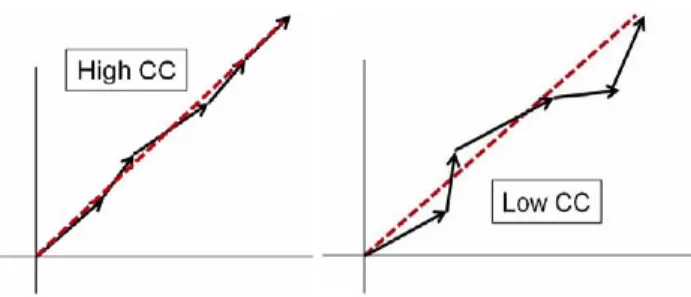
vec-tor) determined by the sum of the cross correlation vectors,H1,2,3V1∗,2,3. The average φDP of all pulses is plotted from the positive x-axis . . . 13 2.4 An example of a cross correlation vector for high CC (left) and low

CC (right) . . . 14 2.5 An example of the radar coverage in Clear Air Mode . . . 15 2.6 An example of the radar coverage in Precipitation Mode . . . 15 2.7 Locations of the Houston LMA sensors (green boxes) in kilometers

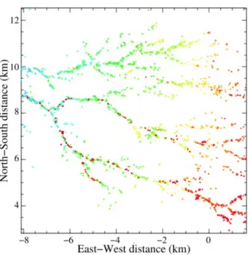
from the center of the LMA network . . . 17 2.8 Plan view of the dendritic structure breakdown of a lightning flash.

Sources show timing of the flash, with cool colors being older detected sources and warmer colors being most recent sources (Thomas et al. 2004) . . . 19 2.9 Schematic representation of the TOA method used to locate VHF

sources for the LMA. The time and location of the arrival of the source at each sensor can be used to solve a system of equations to determine the time and position (x,y,z,t) of the VHF source, where c is the propagation speed of the signal (Thomas et al. 2004) . . . 19

(8)

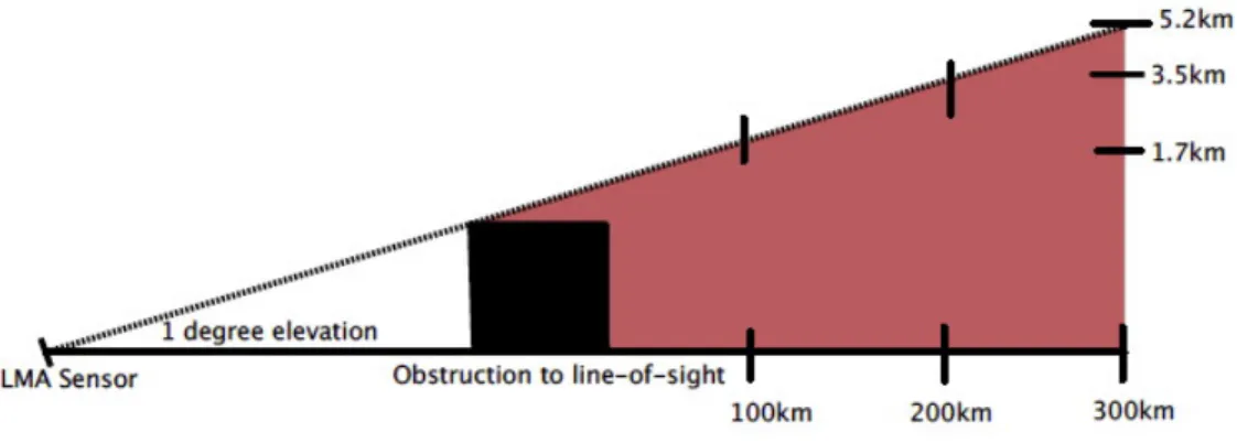
2.10 Schematic illustration of source blockage due to an obstruction in the 1-degree elevation angle. Sources would not be detected in the red shaded area (Cullen 2013) . . . 20 2.11 Map of estimated CG lightning detection efficiency of the NLDN (Buck

et al. 2014) . . . 21 3.1 Pie chart depicting % of cells with only IC lightning, and IC and CG

lightning . . . 26 3.2 Pie chart depicting % of cells with IC lightning as last flash, and CG

lightning as last flash . . . 27 3.3 Reflectivity data on July 13, 2013 for an isolated cell at the -10◦C

level. Distance is in kilometers east (x axis) and north (y axis) from the Houston radar. CG flashes are plotted as black stars, and LMA sources for the cell are recorded for designated times . . . 28 3.4 Next two time steps of cell shown in Figure 3.3. Higher values of

reflectivity are beginning to decrease as the number of sources detected by the LMA are decreasing . . . 29 3.5 Next two time steps of cell shown in Figure 3.4, with the cessation of

lightning occurring in the bottom image . . . 30 3.6 Forecast statistics for the 30 and 35 dBZ thresholds for total lightning

cessation . . . 33 3.7 Forecast statistics for 35 dBZ thresholds and CG lightning cessation . 35 3.8 Differential reflectivity data for the same cell and time as Figure 3.3

at the -10◦C level. Distance is in kilometers east (x axis) and north (y axis) from the Houston radar. CG flashes are plotted as black stars, and LMA sources for the cell are recorded for designated times. Outlined in white is the 30 dBZ reflectivity value . . . 37 3.9 Next two time steps of cell shown in Figure 3.8. The differential

reflectivity in the 30 dBZ region is decreasing as the LMA sources decrease . . . 38 3.10 Next two time steps of cell shown in Figure 3.9, with the cessation of

(9)

3.11 Correlation coefficient data for the same cell and time as Figure 3.3. Distance is in kilometers east (x axis) and north (y axis) from the Houston radar . . . 40 3.12 Next two time steps of cell shown in Figure 3.11 . . . 41 3.13 Next two time steps of cell shown in Figure 3.12 . . . 42 3.14 Timing of differential reflectivity thresholds to the cessation of

light-ning at the -10◦C level . . . 43 3.15 Same as Figure 3.14 expect at -15◦C level . . . 44 3.16 Same as Figure 3.14 expect at -20◦C level . . . 45

(10)

LIST OF TABLES

TABLE Page

1.1 Previous studies conducted on cessation of lightning . . . 7 2.1 2 X 2 contingency table (Mosier et al.2011) . . . . . 23

(11)

1. INTRODUCTION

1.1 Background and Motivation

Lightning is a significant threat to life and property. From 2013 through 2015, there were 75 lightning related fatalities in the United States, four of which occurred in Texas (National Weather Service 2016). Many lightning related fatalities occur during the initiation or dissipation of the most intense lightning period of a thun-derstorm (Holle et al. 1992). The peak months for lightning activity in the United States are June, July and August, which are also some of the peak months for out-door activities (Jensenius 2015). To protect life and property, it becomes imperative to accurately forecast the initiation and cessation of lightning.

Not only is it vital to accurately forecast lightning events for the protection of people’s lives during outdoor activities, it is also important during airfield and space launch operations. During these types of operations, lightning advisories are issued. When a lightning advisory is in place, all operations are halted until the advisory is cancelled. While it is essential to issue lightning advisories with enough lead time for people to reach safety, it is also important to cancel them once the threat of lightning has ended so operations can resume.

Numerous of studies have been conducted on forecasting the initiation of light-ning, but much less have been conducted on the cessation of lightning. With recent advancements in radar and lightning detection, even fewer studies regarding the ces-sation of lightning have been conducted with the most up to date products. Therefore it is critical to begin to develop a reliable forecast technique using the most up to date technology for the cessation of lightning to aid the forecast community.

(12)

(in-cloud (IC) and (in-cloud-to-ground (CG)) observed in thunderstorms. Typically the most dangerous threat to human life is CG lightning, which is lightning that extends from the cloud and reaches the ground. However, for airfield and space launch oper-ations, IC lightning, which is lightning that occurs in cloud only, is also a concern.

When forecasting the cessation of lightning, a forecaster has limited time to make a decision to cancel a lightning advisory. Consequently, the forecaster can only ex-amine a limited number of products. This means complicated algorithms or multiple step forecast techniques do not help when forecasting the cessation of lightning op-erationally. Therefore this study attempts to find a simple, straightforward forecast technique that forecasters can use operationally. Using the most up to date lightning and radar products for the Houston region, this study will examine the cessation of both IC and CG lightning.

1.2 Thunderstorm Electrification

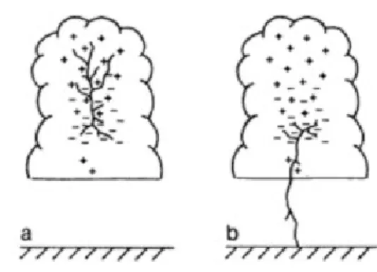
A thunderstorm is defined as “a local storm, invariably produced by a cumulonim-bus cloud and always accompanied by lightning and thunder” (Byers and Braham 1949). For a thunderstorm to in fact be a thunderstorm it must produce light-ning. Lightning is produced when oppositely charged regions form within a storm. Multiple studies have been and are continuing to be conducted to attempt to under-stand the exact processes that cause charged regions and lightning within a thunder-storm. While there are many hypotheses and on-going research regarding this topic, it has been widely accepted that thunderstorms generally develop a tripole structure through micro-physical processes.

The tripole structure in a thunderstorm, which can be seen in Figure 1.1, consists of a small region of positively charge build up at the base of a the cloud, a negatively dominate charge region between the -10 and -20◦C temperature levels, and a positive

(13)

charge region above the -20◦C level (Krehbiel 1986). The positive charge region at the base of the thunderstorm is mainly due to precipitation and latent heat effects. The positive charge region at the top of a thunderstorm forms as ice crystals that are positively charged are carried up by the updraft. While these positive charge regions are important to the overall tripole structure of the thunderstorm, the development of the predominately negative charge region is arguably the most important to the development and cessation of lightning.

Figure 1.1: Tripole structure in a thunderstorm with a.) in-cloud lightning b.) cloud-to-ground lightning (Krehbiel 1986)

There are many theories for the development of the predominately negative charge region between the -10 and -20◦C levels in a thunderstorm. The most widely ac-cepted method for the development of this region in isolated convective cells is the non-inductive graupel-ice collision (NIC) theory, initial proposed by Reynolds et al. (1957), and confirmed by Takahashi (1978) and Saunders et al. (2006). The NIC theory states that in the critical -10 to -20◦C region of a thunderstorm, collisions be-tween supercooled water droplets, ice crystals, and graupel occur along the updraft and downdraft interface. When supercooled water droplets collide with ice crystals,

(14)

the water droplets instantly freeze on the ice crystal upon contact. This process is called riming and creates graupel. The graupel then collides with other ice crystals and results in charge separation between particles. The sign of the charge separa-tion depends on the temperature and the liquid water content of the thunderstorm (Saunders et al. 2006). It is the development of this charge separation in a storm that often results in lightning (Figure 1.1).

This study will not examine further the specifics of the charge separation within a thunderstorm. Further explanation of charge separation processes can be found in the literature mentioned above. The importance of the charge separation for this study was to focus on the presence of graupel and supercooled water droplets between the -10 to -20◦C levels.

1.3 Previous Studies and Forecast Techniques

One of the most reliable and frequently used forecasting tools for the cessation of lightning is the “30-30 rule” (Holle et al. 1999). The first 30 is in relation to the amount of time in seconds between a flash of lightning and the sound of thunder that accompanies it. The time in seconds between the observer seeing a flash of lightning and hearing the accompanying thunder implies the distance of the lightning from the observer. Holle et al. (1999) found that 30 seconds between the flash and thun-der implies that the lightning is 10 km or 6 miles away and poses a low risk that lightning will occur at the observer’s location. The second 30 is in relation to the time in minutes from the last flash of lightning seen or thunder heard. It has been established that 30 minutes after the last occurrence of lightning, it is safe to resume outdoor activities. This method is widely used when canceling lightning advisories or giving the “all clear”. The purpose of many studies when trying to find a new forecast technique is to shorten the wait time of 30 minutes before giving the “all

(15)

clear”.

Reviewing previous studies of lightning initiation can aid in finding forecast tech-niques for the cessation of lightning by reversing the findings. Mosier et al. (2011) examined reflectivity values (30, 35, and 40 dBZ) of 1,028,510 cells that were ob-served in the summer between 1997 and 2006 over the Houston region to develop forecast techniques for the initiation of CG lightning. They found that once the threshold of 30 dBZ was observed at the -20◦C level, CG lightning was expected to occur. This threshold produced a ten minute average lead time before the first CG flash was observed. This study will examine the possibility that using the reflectivity values of 30 and 35 dBZ as thresholds to the cessation of lightning could prove to be useful.

Woodard et al. (2012) was one of the first studies to examine products available from the dual-polarization upgrade of the Next Generation Radar (NEXRAD) net-work (discussed in Section 2.2) in respect to the initiation of total lightning. They studied 31 thunderstorms and 19 non-thunderstorms over northern Alabama by ex-amining reflectivity, differential reflectivity, and fuzzy-logic particle identification. They found that the most reliable forecast technique for the initiation of total light-ning was observing 40 dBZ at the -15◦C level. This technique had an average lead time of eight minutes before the first lightning flash. However, since some agencies such as the Air Force require longer lead times, the added detection of graupel by the fuzzy-logic particle identification at the -15◦C level led to a lead time of 9.5 min-utes. This added criterion produced a slight decrease in the reliability of the forecast technique.

They also examined possible columns of supercooled water droplets, which they called differential reflectivity columns. These columns were denoted by elevated dif-ferential reflectivity values of greater than 1 dB in an area of 40 dBZ or more at the

(16)

-10◦C level. They found that using the presence of a differential reflectivity column as a forecast threshold produced a slight decrease in forecast reliability as compared to reflectivity thresholds alone, but provided an 11 minute lead time. It is possible that reversing the differential reflectivity thresholds defined in Woodard et al. (2012) can aid in forecasting the cessation of lightning.

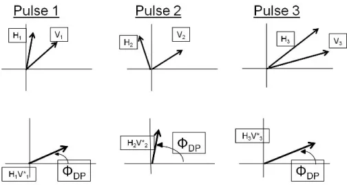
Clements and Orville (2008) conducted a study of 37 isolated cells that occurred between 2005 and 2006 over the Houston region to develop a warning time technique for CG lightning initiation and cessation. In terms of CG cessation, they examined total lightning characteristics and radar reflectivity. They found that total lightning characteristics (IC versus CG occurrences) were not useful in forecasting when the last CG flash would occur. They concluded that when the height of the 45 dBZ reflectivity value fell below the -10◦C level, CG lightning would no longer occur.

Seroka et al. (2012) also examined total lightning characteristics with respect to lightning initiation and cessation. They studied 17,649 cells that developed in the summer months of 2006 through 2009 over the Kennedy Space Center in Florida. They examined reflectivity values (30, 35, and 40 dBZ) to optimize radar-based forecasting of total lightning. They concluded the best thresholds for predicting IC lightning was 25 dBZ at the -15◦C level, and the best predictor of CG lightning was 25 dBZ at the -20◦C level. They also found that 63% of the cells observed had an IC flash as the last lightning event, illustrating that dissipating thunderstorms tend to produce mainly IC lightning and fewer CG flashes before the cessation of total lightning.

A recent study on the cessation of lightning using dual-polarization radar prod-ucts is Preston and Fuelberg (2015) . They examined 40 isolated thunderstorms over the Cape Canaveral area of central Florida for trends in polarimetric radar parame-ters at -10, -15 and -20◦C levels. Results from the 40 storms showed that reflectivity

(17)

thresholds, the presence of graupel (as determined by the hydrometeor classification algorithm (HCA)), and the presence of graupel along with reflectivity thresholds at the -10◦C level proved to be the most promising predictors. Ten independent storms from the data set were then used to further examine the three parameters. From these ten storms it was found that once the presence of graupel and reflectivity of 35 dBZ or greater were no longer observed at the -10◦C level, total lightning has ended. They also studied dual-polarized radar products of differential reflectivity and correlation coefficient in a statistical manner. They preformed correlation tests on these polarimetric parameters in respect to minutes before and after total light-ning cessation. They found that none of the parameters converged toward a certain threshold during the cessation of lightning. One downfall to this approach is the lack of combining dual-polarization products such as differential reflectivity with reflec-tivity to better identify the presence of graupel and supercooled water droplets.

A table of previous studies conducted using radar data to determine a forecast technique for the cessation of lightning is provided in Table 1.1. As is evident in Table 1.1, past studies on the cessation of lightning are limited in number and sam-pling of different regions. This warrants continued investigations into operational assessments of lightning cessation using radar products.

(18)

1.4 Research Objectives

The objective of this study is to find a radar-derived forecast technique for the cessation of lightning for isolated, short-lived thunderstorms over the Houston re-gion. This study seeks to provide an in depth look into isolated thunderstorms to examine polarimetric parameters of reflectivity, differential reflectivity, and correla-tion coefficient for the presence of graupel and supercooled water droplets in relacorrela-tion to the cessation of lightning. The goal is to find when a polarimetric radar parameter becomes less and remains less than a defined threshold, which will allow forecasters to quickly and more confidently determine when the threat for lightning has ended. In addition to finding thresholds for the cessation of lightning, this study also looks to examine the timing between the last IC lightning and CG lightning. Typ-ically in a dissipating thunderstorm, the last lightning event will be an IC flash (Clements and Orville 2008). The end time of each lightning event (CG and IC) will be recorded and, if available, the timing difference will be calculated. These results will also be compared to the polarimetric parameter thresholds found to examine if the thresholds change for CG and IC lightning cessation.

(19)

2. DATA AND METHODOLOGY

2.1 Methodology Overview

The important charge separation levels of -10, -15, and -20◦C are examined. Each level will be evaluated to determine the best threshold values of reflectivity and differential reflectivity to predict the cessation of lightning. Correlation coefficient will be used to determine the quality of the dual-polarization data. The reliability of forecast techniques are determined by the calculation of Probability of Detection (POD), Probability of False Alarm (POFA), and Critical Success Index (CSI). Lead time, or wait time, will also be calculated for the polarimetric parameter thresholds to determine if the parameter provides a better predictor of the cessation of lightning than other listed forecast techniques. Lead time will be used to denote time leading up to the last flash of lightning, and wait time will be used to denote time after the last lightning flash. It is important to note that in this study lead time, or wait time, is calculated by using the time of the start of the radar scan that no longer shows the specific threshold, and the time of the last lightning event. This calculation is consistent with previous studies (Clements and Orville 2008; Mosier et al. 2011; Seroka et al. 2012; Woodard et al. 2012; Preston and Fuelberg 2015). However, in actual operations, this calculated time becomes longer as a forecaster must wait for the time it takes for the radar to complete and process the volume scan.

2.2 Radar Data

The Houston Weather Surveillance Radar-1988 Doppler operated by the National Weather Service (NWS) is part of the Next Generation Radar (NEXRAD) network. The NEXRAD network consists of 160 radar sites throughout the United States, 122 that are operated by the NWS. Archived Level-II NEXRAD radar data from the

(20)

Houston radar were obtained for the summer months (June, July, and August) of 2013 through 2015 from the National Climatic Data Center.

Radars operate by transmitting a pulse of radio waves into the atmosphere that reflect off objects and travel back to the radar. From these returns the radar can directly measure reflectivity, radial velocity, and spectrum width, also called base products. Base products are products that the radar directly measures. The radar can then take the base products and create a multitude of derived products.

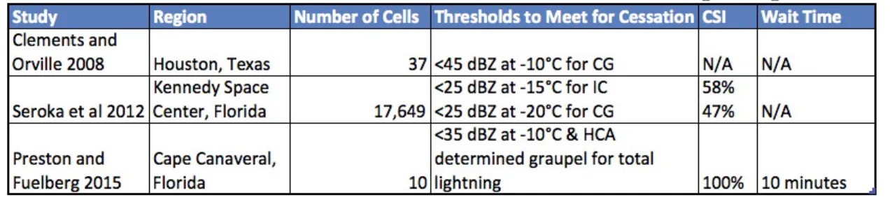
In 2011, the deployment process of upgrading the entire NEXRAD network to dual-polarization began. Previously, the NEXRAD network were single-polarized radars, meaning they only transmitted and received radio waves in the horizontal. The dual-polarization upgrade allows for transmission of simultaneous radio signals in the horizontal and the vertical (Figure 2.1), adding to the amount of products the radar can produce (Istok et al. 2009). This upgrade added differential reflectivity, correlation coefficient, and differential phase to the base products of the radar. The Houston radar began activation of the dual-polarization upgrade on January 21, 2013.

The first base product this study examines is standard horizontal reflectivity (Zh). The radar directly measures Zh by measuring the strength of the horizontal

return signal. Horizontal reflectivity is calculated by the following simplified version of the Probert-Jones equation shown below

Zh =PrR2/CrLa (2.1)

where Zh is the target reflectivity, Pr is the power returned to the radar from the

target in Watts, R is the target range, La is attenuation factor, andCr is the radar

(21)

trans-Figure 2.1: Schematic of transmitting radio signals for single-polarized radars (left) and dual-polarized radars (right)

mitted energy wavelength (Weather Decision Training Branch 2011). In order to easily display horizontal reflectivity for operational use, a logarithmic conversion is applied to Zh such that

Z = 10log10(Zh) (2.2)

where Z is expressed in units of dBZ, or decibels of energy reflected back to the radar. Horizontal reflectivity will be referred to as reflectivity in this study.

The second base product this study examines is differential reflectivity (ZDR). Differential reflectivity is defined as the ratio of the horizontal (Zh) and vertical (Zv)

reflectivity returns expressed in decibels (dB) (Weather Decision Training Branch 2011). This product was used in this study to help describe the shape of the hy-drometeors. A value of 0 dB would imply circular shaped hydrometeors such as hail, and a value of 1.5 dB would imply a more oblique shaped hydrometeor such as a rain drop. It has also been found that a slightly negative value such as -0.5 dB can be indicative of graupel (Evaristo et al. 2013). Using the Probert-Jones equation to

(22)

calculate Zh and Zv respectively, differential reflectivity is calculated as follows

ZDR= 10log10(Zh/Zv) (2.3)

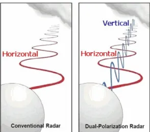
The third base product this study examines is correlation coefficient (CC). Cor-relation coefficient is defined as the consistency of the horizontal and vertical power and phase returns of each pulse (Weather Decision Training Branch 2011). This product helps determine the quality of the base data along with implied information about the overall composition of the hydrometeors. The correlation coefficient is de-termined by the sum cross correlation vector and the average power of the horizontal and vertical signals. The cross correlation vector is calculated for each pulse sepa-rately. It is calculated by evaluating the transmission of the horizontal and vertical signals and measures the similarity between them. Further explanation of the cross correlation vector can be found in Bringi and Chandrasekar (2001) in section 6.4, and a simplified illustration is seen in Figure 2.2. The sum cross correlation vector is then determined by taking the sum of the cross correlation vectors for a series of pulses (Figure 2.3). The correlation coefficient is calculated by taking the length of the sum cross correlation vector, Rhh,vv, and dividing it by the average power of the

horizontal, Ph and verticalPv signals as shown below.

CC =Rhh,vv/(PhPv)(1/2) (2.4)

Correlation Coefficient is expressed as a number between zero and one. A number close to zero (but never exactly zero), or low correlation coefficient, means little correlation between hydrometeors, and a number close to one (but never exactly one), or high correlation coefficient, means near perfect consistency between hydrometeors.

(23)

Figure 2.2: Horizontal and vertical signal vectors from three sample pulses are shown in the top row. H1,2,3 is the horizontal signal vector,V1,2,3is the vertical signal vector. The bottom row shows the calculated cross correlation vector, H1,2,3V1∗,2,3, for each pulse (the asterisk denotes the complex conjugate) andφDP is the angle between the

horizontal and vertical signal vectors denoted from the positive x-axis

Figure 2.3: An example of the sum cross correlation vectorRhh,vv(red dashed vector)

determined by the sum of the cross correlation vectors, H1,2,3V1∗,2,3. The averageφDP

(24)

An example of high correlation coefficient would be when pure rain is being sampled; the correlation coefficient would be close to one. If a hail core composed of different sized hail was being sampled, then the correlation coefficient would be low or closer to zero (Figure 2.4).

Figure 2.4: An example of a cross correlation vector for high CC (left) and low CC (right)

The NEXRAD radars scan the atmosphere in Volume Coverage Patterns (VCPs). VCPs are automated repetitive 360◦ scans of the atmosphere at predefined elevation angles. There are two main operating states, Clear Air Mode (Figure 2.5) and Precipitation Mode (Figure 2.6). There are two Clear Air Mode VCPs and seven Precipitation Mode VCPs. The selection of which VCP the Houston radar is set to is controlled by the NWS Houston/Galveston Weather Forecast Office. When precipitation is occurring within the range of the radar beam, the Weather Forecast Office switches the VCP to one of the Precipitation Modes. This study did not include or exclude any radar data based solely on which VCP the radar was operating. In operational forecasting, the forecaster is subjected to the Weather Forecast Office’s choice of VCP. Thus, for this study to properly emulate conditions subject to an operational forecaster, radar data were not filtered based on VCPs.

(25)

Figure 2.5: An example of the radar coverage in Clear Air Mode

Figure 2.6: An example of the radar coverage in Precipitation Mode

As the radar scans the atmosphere, the beam increases or decreases in height as it travels away from the radar due to the curvature of the earth, refractivity of the atmosphere, and other factors. For better examination of the radar data at specific levels, the radar data were converted to constant altitude plan projection indicator (CAPPI) format. First, the radar files were converted to Universal Format using the Radx program developed by the National Center for Atmospheric Research. Then the Universal Format radar files were converted to CAPPI using the same program, by taking the PPI data and interpolating it onto a 400 x 400 km horizontal and 20 km vertical Cartesian grid. The resolution for the radar in both the horizontal and the vertical is 1 km. Mosier et al. (2011) compared 0.5 and 1 km vertical resolution over the Houston region to determine the best resolution. He found that there was not a significant difference between the 0.5 and 1 km resolution, but that the 1 km was more useful than the 0.5 km resolution when applying the Storm Cell Identifi-cation and Tracking (SCIT) algorithm. Therefore a resolution of 1 km was used.

(26)

Once the radar files were converted to CAPPI, a modified version of SCIT was applied to identify and supply information on individual storm cells. The SCIT al-gorithm was chosen for this study as the NWS also uses a version of SCIT in real time to track cells. The algorithm used in this study was obtained from Mosier et al. (2011). They modified the original SCIT algorithm in order to apply it to radar data that is in CAPPI format. The CAPPI-SCIT algorithm contains four steps: identification of storm cell one-dimensional segments, creation of three-dimensional storm cells and calculating storm centroids, storm tracking, and storm position fore-casting. For this study, only the first two steps were used to help identify isolated thunderstorms. The steps to the CAPPI-SCIT algorithm are outlined in more detail in Mosier et al. (2011).

2.3 Lightning Data

To appropriately develop a forecast technique for the cessation of lightning, prod-ucts that allow for observation of total lightning (IC and CG lightning) are required. The Houston Lightning Mapping Array (LMA) is used to examine IC lightning, and the National Lightning Detection Network (NLDN) is used to examine CG lightning.

2.3.a Houston Lightning Mapping Array

The Houston LMA was developed by New Mexico Institute of Mining and Tech-nology and was purchased by Texas A&M University. The Houston LMA was in-stalled in April 2012 and is composed of 12 Very High Frequency (VHF), time of arrival (TOA) ground sensors. Ten of the sensors are surrounding the downtown Houston region, with two outlying sensors to the northwest (College Station, TX) and the southeast (Galveston, TX) of Houston. The network measures 150 km from north to south, with the center located at 29.76 N, 95.37 W (Figure 2.7).

(27)

Figure 2.7: Locations of the Houston LMA sensors (green boxes) in kilometers from the center of the LMA network

60 to 66 MHz range during the electrical breakdown and propagation of a lightning flash (Cullen 2013). This results in multiple sources that are recorded for a single lightning flash (Figure 2.8). The sensors record the location (x,y,z) and time of each source using the TOA technique shown in Figure 2.9 and outlined in further detail in Thomas et al. (2004). For the Houston LMA, a minimum of six sensors need to detect a source to accurately determine the TOA. This minimum sensor requirement allows for a reduced chi-square value, or a measure of a goodness of fit, of no more

(28)

than five.

The Houston LMA data that were used for this study contained the following information for each individual source: time to the nanosecond, latitude, longitude, altitude, reduced chi-square, received power, and a station mask that describes which sensors detected the source. This study focused on the time, latitude, and longitude of each source, and tailored the reduced-chi squared. Personal correspondence with Dr. Krehbiel (2015), a professor at New Mexico Technical Institute, revealed that reducing the max allowed reduced chi-square from five to one will eliminate most of the noise-contaminated solutions.

Since the network detects the VHF emissions from a lightning flash and can plot the individual sources (Figure 2.8), it is able to detect both CG and IC lightning. However, there are some limitations with the range of detection. Cullen (2013) tested the effective range of the Houston LMA by examining case studies for the region. He found when all 12 sensors are operational, the effective two dimensional range (x,y) of the network is 250 km from the center, and when the minimum amount of sensors are operational, that range decreases to just over 140 km. In respect to the vertical range resolution of the Houston LMA, the curvature of the Earth causes source detection at lower levels to become impossible beyond 100 km from the center of the network. Additionally, with the line of sight of each sensor starting at one degree elevation, obstructions to the line of sight (such as buildings) would hinder the detection of low level sources (Figure 2.10). With this in consideration, the range of detection of low level sources (about 5 km in elevation) is 50 km from the center of the network.

The vertical resolution range of the LMA becomes a problem in this study when using LMA data to determine CG lightning. Radar data are vital in this study, and therefore coinciding complete data of the radar and LMA are needed. With the

(29)

Figure 2.8: Plan view of the dendritic structure breakdown of a lightning flash. Sources show timing of the flash, with cool colors being older detected sources and warmer colors being most recent sources (Thomas et al. 2004)

Figure 2.9: Schematic representation of the TOA method used to locate VHF sources for the LMA. The time and location of the arrival of the source at each sensor can be used to solve a system of equations to determine the time and position (x,y,z,t) of the VHF source, where c is the propagation speed of the signal (Thomas et al. 2004)

(30)

Figure 2.10: Schematic illustration of source blockage due to an obstruction in the 1-degree elevation angle. Sources would not be detected in the red shaded area (Cullen 2013)

radar only 43 km south of the LMA network center, the cone of silence resulting in limited higher elevation scan coverage, as shown in Figure 2.6, would prevent proper upper level radar data of thunderstorms that are close enough to the LMA network to detect CG lightning to be considered for this study. Due to these limitations, adding in CG lightning data from the NLDN are required.

2.3.b National Lightning Detection Network

The NLDN is operated and managed by the Vaisala Thunderstorm Unit located in Tucson, Arizona (Biagi et al. 2007). Complete coverage of CG lightning through-out the continental United States is provided by the network. The NLDN has been operational for the continental United States since 1989, with the most recent up-grades completed in August of 2013.

The NLDN is composed of ground-based LS7002 sensors developed by Vaisala that detect low frequency (LF) and very low frequency (VLF) electromagnetic radia-tion (1-350 kHz) produced by CG lightning (Mallick et al. 2014). Vertically-polarized transient pulses are emitted from lightning that strikes the ground and these

(31)

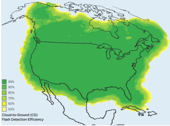
emit-ted pulses travel along the surface of the earth. The sensors detect these pulses and use onset corrections to determine accurate location and timing of an event (Nag et al. 2014). The data are then sent to Vaisala’s Network Control Center where it is processed using the Total Lightning Processor. The processed data allows for a 95% efficiency detection of CG lightning within the network (Figure 2.11).

The NLDN data used in this study consists of date, time, location, polarity,

Figure 2.11: Map of estimated CG lightning detection efficiency of the NLDN (Buck et al. 2014)

lightning type (CG or IC), and elevation. This study focuses only on the time and location of the CG lightning (an elevation of zero). The upgrade completed on the NLDN during the summer of 2013 does not affect the consistency of the data for

(32)

this study. The upgrade was to improve detection of IC lightning. This study does not use the NLDN to determine IC lightning strikes and therefore the data set is not affected.

2.4 Sounding Data

Observed upper air soundings are critical for this study in order to identify the height of the -10, -15, and -20◦C levels. Most forecasters use observed sounding data in order to gain an image of the atmospheric profile. Unfortunately, Houston does not launch a radiosonde used to create an observed sounding. Therefore, a weighted sounding was created for the Houston region from observed sounding data from Lake Charles (LCH), Corpus Christi (CRP), and Fort Worth (FWD). The observed sounding data were obtained from the Earth System Research Laboratory Radiosonde Database. LCH is located 194 km east of Houston, CRP is 302 km southwest of Houston, and FWD is 404 km north-northwest of Houston.

The weighted average sounding algorithm was obtained from Mosier et al. (2011). A 00 UTC and a 12 UTC Houston sounding was created for each day used in the study with LCH weighted most heavily, followed by CRP, then FWD. The observed sounding that was created closest to the studied event time was used (e.g.. event time of 22 UTC on June 3 used a 00 UTC sounding from June 4). This give the best estimate of the atmospheric conditions. Model soundings were not used in this study to maintain consistency of weighted sounding data, and to eliminate the issue of erroneous or biased model data.

2.5 Forecast Statistics

When researching forecast techniques in meteorology, there are many statistics that are created to determine the accuracy of each technique. A few of them are Probability of Detection (POD), Probability of a False Alarm (POFA) (also referred

(33)

to in other literature as False Alarm Ratio), and Critical Success Index (CSI). All of these statistics can aid in understanding the reliability of a forecast technique, and are calculated for this study.

In order to calculate these statistics, two questions must be answered. First, was the event forecasted, and second, was the event observed. This is done by using a schematic 2 X 2 contingency table (Table 2.1). For this study, the first question is answered if the thresholds described in this study are met or not. From there, if the first question’s answer is yes, the second question is if the lightning did in fact end with the thresholds being met (box X) or if the lightning continued after the thresholds were met (box Y). If the first question’s answer is no, then the second question is automatically answered as yes since all cases in this study had lightning occur (box Z). The no forecast/no event cases were not applicable in this study (box W).

Table 2.1: 2 X 2 contingency table (Mosier etal.2011)

POD and POFA are the most common used in forecast literature. POD cal-culates a percentage on how frequently the technique predicted an observed event. Mathematically POD is determined by

(34)

A POD of 100% would mean that the technique correctly forecasted every observed event. POFA is a percentage of non-successful forecast events to total events fore-casted, or how frequently the forecast technique produced a false alarm. Mathemat-ically POFA is determined by

P OF A=Z/(X+Z) (2.6)

The goal is to keep POD high and POFA low. This would result in the most accurate forecast technique. However, POD is skewed to only considering observed events, which is not the case when dealing with real world forecasting. Therefore CSI is used as a better indicator of how the forecast technique would perform when all events are considered.

CSI is defined as the percentage of correct forecasts to the total number of events (observed and false alarms). It is mathematically defined as

CSI =X/(X+Y +Z) (2.7)

CSI differs from POD by factoring in a forecasted non-event. CSI gives better insight to how the forecast technique works overall as it factors in false alarms. Having a high CSI is desired as it suggests the forecast technique works well when all event types are considered. To keep with consistency of other previous published literature, CSI was used as a primary indicator of the reliability and overall skill of the forecast technique. Caution should be taken when comparing CSI scores from studies conducted in different environments as the frequency of events differs in each study.

(35)

2.6 Analysis Process

Isolated, short-lived thunderstorms that dissipated in a 400 km box centered on the Houston radar were chosen for this study. Thunderstorms that developed or dissipated over the Gulf of Mexico were excluded from this study. Thunderstorms were chosen based on their data availability at upper levels (6 to 9 km), and the entire thunderstorm must have initiated and dissipated within the bounds of the study. With the center of the LMA network located 43 km north of the Houston radar, all storms included in this study were in the effective range of 140 km for LMA detection.

Steps used in this study are as follows: 1) identify isolated thunderstorms, 2) de-termine the timing of the last CG and/or IC lightning event, 3) create an averaged observed Houston sounding to find the -10, -15, and -20◦C levels, 4) examine the reflectivity, differential reflectivity, and correlation coefficient radar data correspond-ing with the timcorrespond-ing of the cessation of lightncorrespond-ing at the -10, -15 and -20◦C levels, 5) record timing of polarimetric thresholds, 6) calculate POD, POFA, and CSI for parameter thresholds, and 7) calculate timing difference of CG and IC lightning and compare to polarimetric parameter thresholds.

(36)

3. RESULTS

3.1 Overview

A total of 42 isolated cells were examined in the summer months of 2013 through 2015. Fifteen of those cells were observed in 2013, thirteen were observed in 2014, and fourteen were observed in 2015. Out of the 42 cells, 35 produced both IC and CG lightning and seven cells produced just IC lightning (Figure 3.1). Out of the 35 cells that produced both IC and CG lightning, four of those cells’ last lightning event was a CG flash while the remaining 31 cells produced an IC flash as the last lightning event (Figure 3.2). These findings are similar to results found in Clements and Orville (2008) who recorded that 70% of the cases they observed had IC lightning as the last lightning event. The average time between the last CG and IC flash found in this study is 8 minutes and 11 seconds.

Figure 3.1: Pie chart depicting % of cells with only IC lightning, and IC and CG lightning

(37)

Figure 3.2: Pie chart depicting % of cells with IC lightning as last flash, and CG lightning as last flash

Reflectivity, differential reflectivity, and correlation coefficient were examined to find if specific thresholds of each parameter aided in forecasting the cessation of light-ning. The timing of radar data studied for each observed cell began at a minimum of two volumes scans prior to the last CG flash (or IC flash if there was no CG), and ended when the 25 dBZ height dropped below the -10◦C level, or 30 minutes after the last flash (whichever came first).

3.2 Reflectivity Thresholds

Reversing the findings of Mosier et al. (2011), the 30 and 35 dBZ values were examined as thresholds to the cessation of lightning. These reflectivity thresholds were examined at the -10, -15, and -20◦C levels. An example of the cessation of lightning for an isolated cell as seen in reflectivity data at the -10◦C level is shown in Figures 3.3 to 3.5.

(38)

Figure 3.3: Reflectivity data on July 13, 2013 for an isolated cell at the -10◦C level. Distance is in kilometers east (x axis) and north (y axis) from the Houston radar. CG flashes are plotted as black stars, and LMA sources for the cell are recorded for designated times

(39)

Figure 3.4: Next two time steps of cell shown in Figure 3.3. Higher values of reflec-tivity are beginning to decrease as the number of sources detected by the LMA are decreasing

(40)

Figure 3.5: Next two time steps of cell shown in Figure 3.4, with the cessation of lightning occurring in the bottom image

(41)

3.2.a Total Lightning Cessation

First, the -10◦C level was studied. A hit (box X in Table 2.1) was noted when the reflectivity thresholds decreased after the last lightning flash, a miss (box Y in Table 2.1) was noted when the reflectivity thresholds decreased before the last lightning flash, and a false alarm (box Z in Table 2.1) was noted when the thresholds never decreased during the time frame of the observed cell. The POD, POFA and CSI for the 30 dBZ threshold at this level were found to be 94%, 19%, and 77% respectively. The POD, POFA and CSI for the 35 dBZ threshold were calculated to be 59%, 8%, and 56%. It is clear that the 30 dBZ threshold is a much more reliable parameter with a CSI that is nearly 20% higher than the 35 dBZ threshold. The average wait time between the last lightning flash and the first volume scan that the 30 dBZ threshold was no longer observed at this level is 7 minutes and 30 seconds.

In order to be confident that the 30 dBZ threshold was in fact met, this study found if the 30 dBZ value was not observed for at least two volumes scans, it was likely to not occur again during the dissipation of the cell. In actual operations, a forecaster waiting for two volume scans would wait an average of 8 to 12 minutes for the radar to complete the scan and process the data. Adding the average time it takes for the radar data to process to the average wait time found at the -10◦C level for the 30 dBZ threshold equates to an average of 15 to 20 minutes. Using the maximum end of this timing, this technique would be about 10 minutes faster than waiting 30 minutes from the last lightning flash using the “30-30 rule”.

The low POD and CSI of the 35 dBZ threshold mainly indicates that the 35 dBZ threshold decreased below the -10◦C level before the last flash of lightning (excluding the one case where the 35 dBZ was never reached at the -10◦C level). However, with the POD and CSI calculated at about 50%, this means half of the time for the

(42)

cases observed the 35 dBZ threshold was met after lightning ended. These findings show that this threshold would not be reliable to use for a lead time or a wait time technique for total lightning cessation.

Moving to the -15◦C level, the same methods used to examine the -10◦C level were used. The 30 dBZ threshold forecast statistics were found to be a POD of 88%, a POFA of 8%, and a CSI of 82%. The 35 dBZ threshold forecast statistics were found to be a POD of 46%, POFA of 5%, and a CSI of 45%. As seen at the -10◦C level, the 30 dBZ threshold is much more reliable than the 35 dBZ threshold. However, the 30 dBZ threshold shows a higher CSI at the -15◦C level than at the -10◦C level. The average wait time between the last flash of lightning and the 30 dBZ threshold at the -15◦C level is 6 minutes and 57 seconds.

Finally, the -20◦C level is examined for the 30 and 35 dBZ thresholds using the same methods as the -10 and -15◦C levels. The 30 dBZ threshold shows a POD of 73%, POFA of 9%, and a CSI of 68%. The 35 dBZ threshold shows a POD of 44%, POFA of 5%, and a CSI of 44%. Again statistics show the 30 dBZ threshold is a much better technique in terms of reliability than the 35 dBZ threshold. The average wait time between the last flash of lightning and the 30 dBZ threshold at this level is 8 minutes and 41 seconds. However, the 30 dBZ threshold at the -20◦C level shows a lower POD and CSI as compared to statistics calculated at the -10 and -15◦C levels. POD, POFA, and CSI for the 30 and 35 dBZ threshold at every level is presented in Figure 3.6. At first glance, the 30 dBZ threshold at the -10◦C level seems to be the best indicator of the cessation of lightning. However, while the 30 dBZ threshold at the -10◦C level has the highest POD, it also has the highest POFA and second highest CSI score. Therefore, taking all forecast statistics into account, the 30 dBZ threshold at the -15◦C level proves to be the best performing forecast technique with the highest CSI score, the second highest POD score, the second lowest POFA score,

(43)

and shortest average wait time.

Figure 3.6: Forecast statistics for the 30 and 35 dBZ thresholds for total lightning cessation

3.2.b CG Lightning Cessation

As mentioned previously, 88% of the cases that produced both IC and CG light-ning had an IC flash as the last flash. Therefore, CG lightlight-ning typical occurs before the last IC flash. With the 35 dBZ threshold proving to be unreliable in forecasting total lightning cessation, it is worth examining if this threshold aids in forecasting the last CG flash.

The -10, -15 and -20◦C levels were examined separately for the 35 dBZ threshold in respect to the last CG flash. A hit (box X in Table 2.1) was noted when the 35

(44)

dBZ threshold decreased after the last CG flash, a miss (box Y in Table 2.1) was noted when the 35 dBZ threshold decreased before the last CG flash or if the 35 dBZ threshold was never reached, and a false alarm (box Z in Table 2.1) was noted when the 35 dBZ threshold never decreased during the time frame of the observed cell.

For the -10◦C level, the POD is calculated to be 94%, the POFA is 5%, the CSI is 89%. The average wait time between the last observed 35 dBZ value and the last CG lightning is 12 minutes and 5 seconds. For the -15◦C level, the POD is calculated to be 83%, the POFA is 3%, and the CSI is 81%, and the average wait time is 9 minutes and 8 seconds. Lastly for the -20◦C level, the POD is 76%, the POFA is 0%, and the CSI is 76%, with an average wait time of 10 minutes and 42 seconds. All forecast statistics for each level are shown in Figure 3.7. As the figure shows, the best forecast technique for the last CG flash is 35 dBZ decreasing below, and remaining below, the -10◦C level as it has the highest POD and CSI.

It was found that a minimum of two volume scans in which the 35 dBZ threshold was no longer observed provides sufficient evidence that the 35 dBZ value will no longer occur during the dissipation of the cell. As stated previously, this equates to an average wait time of 8 to 12 minutes for the radar data to process. Adding this wait time to the average wait time of the 35 dBZ threshold at -10◦C level equates to about 24 minutes before it would be safe to assume no CG lightning is expected.

3.3 Dual-Polarized Radar Products

Dual-polarized radar products of correlation coefficient and differential reflectivity were also studied. Correlation coefficient was used to confirm reliability of differential reflectivity data, and all data showing a correlation coefficient of less than 0.94 was not considered. Differential reflectivity aids in determining types of hydrometeors by detecting their shape, and this study looks to focus on the presence of graupel and

(45)

Figure 3.7: Forecast statistics for 35 dBZ thresholds and CG lightning cessation

supercooled water droplets. To determine possible graupel presence, a differential reflectivity value of -0.5 dB observed in a region of greater than or equal to 30 dBZ criteria was used (Evaristo et al. 2013). Using a method similar to the differential reflectivity column defined in Woodard et al. (2012), supercooled water droplets are determined by observing 0.5, 1, and 1.5 dB in an area of 30 dBZ or greater. Since findings in this study show that the 30 dBZ threshold usually decreases several minutes after the cessation of lightning, the hypothesis is that specific differential reflectivity thresholds would decrease before the 30 dBZ threshold and could be indicators to the cessation of lightning.

The -0.5, 0.5, 1, and 1.5 dB differential reflectivity values observed in an area of 30 dBZ or greater were examined at the -10, -15, and -20◦C levels. The timing of the thresholds were calculated based on the timing of the start of the first radar scan

(46)

that showed the differential reflectivity had decreased below and remained below the denoted value. An example of differential reflectivity values during the cessation of lightning for a cell is shown in Figures 3.8 to 3.10. The correlation coefficient for the same cell and timing is shown in Figures 3.11 to 3.13.

3.3.a Specific Differential Reflectivity Thresholds

First, each differential reflectivity threshold was examined at the -10, -15, and -20◦C levels individual. Starting at the -10◦C level, it was found that out of 42 ob-served isolated cells, on average 21 cells showed steady, reliable differential reflectivity values. This excludes cells that never met the differential reflectivity thresholds, dif-ferential reflectivity thresholds that only appeared for one radar scan, or thresholds that were met because the 30 dBZ threshold decreased, meaning the differential re-flectivity values did not decrease beforehand as hypothesized. Only cells that showed steady, reliable differential reflectivity values were used to calculate lead time to the cessation of lightning.

Out of the reliable cells, on average all the differential reflectivity thresholds de-creased before the cessation of lightning 14 times, and after the cessation of lightning seven times. The results of the reliable cells’ differential reflectivity values at the -10◦C level are shown in Figure 3.14. As the figure shows, there is not a tight grouping of a specific differential reflectivity threshold at a time leading to, or after, the cessa-tion of lightning. Therefore no forecast statistics were calculated for the thresholds at this level.

Next, the -15 and -20◦C levels were examined. At both of these levels, the -0.5 and 0.5 dB values were observed about twice as often as the 1 and 1.5 dB values. These results are to be expected as higher values of differential reflectivity are associated with large rain drops, and large rain drops at such cold temperatures are uncommon.

(47)

Figure 3.8: Differential reflectivity data for the same cell and time as Figure 3.3 at the -10◦C level. Distance is in kilometers east (x axis) and north (y axis) from the Houston radar. CG flashes are plotted as black stars, and LMA sources for the cell are recorded for designated times. Outlined in white is the 30 dBZ reflectivity value

(48)

Figure 3.9: Next two time steps of cell shown in Figure 3.8. The differential reflec-tivity in the 30 dBZ region is decreasing as the LMA sources decrease

(49)

Figure 3.10: Next two time steps of cell shown in Figure 3.9, with the cessation of lightning occurring in the last image

(50)

Figure 3.11: Correlation coefficient data for the same cell and time as Figure 3.3. Distance is in kilometers east (x axis) and north (y axis) from the Houston radar

(51)

(52)

(53)

Figure 3.14: Timing of differential reflectivity thresholds to the cessation of lightning at the -10◦C level

The -0.5 and 0.5 dB thresholds at the -15◦C level were found reliable (using the same method at the -10◦C level) for 24 cases and at the -20◦C level were found reliable for 20 cases. The 1 and 1.5 dB thresholds at the -15◦C level were found reliable for 12 cases and at the -20◦C level for four cases.

The results of the reliable differential reflectivity values at the -15 and -20◦C levels are shown in Figure 3.15 and 3.16. Again as the figures show, there is not much indication of tight grouping of a specific threshold at a time before or after the cessation of lightning. The -0.5 dB value at the -15◦C level shows some promise with a gathering between the zero and 10 minute time frame before cessation, and is examined further.

(54)

Figure 3.15: Same as Figure 3.14 expect at -15◦C level

A total of 25 cells showed reliable data for the -0.5 dB differential reflectivity threshold at the -15◦C level. Out of the 25 cells, 17 cells had the threshold decrease before the last lightning flash, and seven after the last lightning flash. To determine forecast statistics for this threshold, a hit (box X in Table 2.1) was noted when the threshold decreased before the cessation of lightning, a miss (box Y in Table 2.1) was noted when the threshold decreased after the cessation of lightning, and a false alarm (box Z in Table 2.1) was noted when the threshold never decreased during the time frame the cell was observed. The forecast statistics equate to a POD of 71%, a POFA of 6%, and a CSI of 68%. With a fairly low CSI, and factoring that only 60% of the total storms sampled in this study were included in this calculation, there is not much confidence placed in this threshold to forecast the cessation of lightning.

(55)

Figure 3.16: Same as Figure 3.14 expect at -20◦C level

3.3.b Total Differential Reflectivity Thresholds

With examination of specific differential reflectivity thresholds showing no indi-cation to aid in the forecast of the cessation of lightning, each cell was examined individually with respect to all differential reflectivity thresholds. If all differential reflectivity thresholds were no longer observed for a cell, indicating graupel and su-percooled water droplets were no longer present, this could aid in forecasting the cessation of lightning.

First, each of the 42 cells were analyzed and the time was recorded when all the differential reflectivity thresholds at every level were no longer observed. It was found that 14 cells had all thresholds decrease before the cessation of lightning, and the other 28 cells had at least one threshold that decreased after. This finding is a

(56)

negative result to the hypothesis that the differential reflectivity thresholds will be met before the cessation of lightning. This is mostly due to the thresholds being met with the decrease of the 30 dBZ reflectivity value, and not a specific indication of the differential reflectivity thresholds.

Finally, all 42 cells were studied at the -10, -15, and -20◦C levels individually to determine if a decrease of all differential reflectivity thresholds at these levels can be a predictor of the cessation of lightning. At the -10◦C level, 16 cells had all differ-ential reflectivity thresholds decrease before the last lightning flash and 26 decrease after. At the -15◦C level, 20 cells had all differential reflectivity thresholds decrease before the last lightning flash and 20 after. The remaining two cells at this level never reached the indicated differential reflectivity thresholds. At the -20◦C level, 22 cells had all differential reflectivity thresholds decrease before the last lightning flash and 16 that decreased after. The remaining 4 cells never met the differential reflectivity threshold values. As there is no large percentage of thresholds decreasing before or after the cessation of lightning, none of these results indicate a technique that can be used to forecast the cessation of lightning.

(57)

4. CONCLUSIONS

4.1 Conclusions

Previous research has been conducted to understand and attempt to forecast the cessation of lightning using radar data. This study adds to previous research by ex-amining reflectivity thresholds and the cessation of total lightning over the Houston region, and to delve further into dual-polarized base radar data. This study also examines total lightning to optimize forecasting the last CG and IC flash. A total of 42 isolated cells that dissipated over the Houston region in the summer months of 2013 through 2015 were examined. Of those 42 cells, 88% produced both IC and CG lightning, and 17% produced only IC lightning.

The best forecast technique for the cessation of total lightning (IC and CG) was found to be the 30 dBZ reflectivity value decreasing below the -15◦C level. Forecast statistics prove that this technique had a POD of 88%, a POFA of 8%, and a CSI of 82%. This technique had the highest CSI, marking it the most reliable. The wait time calculated from the last lightning flash to the time of the first radar scan that did not show a reflectivity of 30 dBZ or greater at the -15◦C level is about 7 minutes. This is comparable to other studies of lightning cessation such as Seroka et al. (2012) and Preston and Fuelberg (2015).

The technique found in Seroka et al. (2012) of 25 dBZ decreasing below the -15◦C level had a much lower CSI at 58%. As stated in Section 2.5, caution should be taken when comparing CSI scores of different data sets. Differences could be accounted for by the climatology of the region and general synoptic set up, as Florida is much more influenced by a sea breeze. However, Seroka et al. (2012) developed this threshold for initiation and cessation of lightning. It is likely that a higher CSI score can come

(58)

from a technique developed solely for forecasting lightning cessation, which is what was developed in this study.

The technique found in Preston and Fuelberg (2015) of 35 dBZ and HCA de-termined graupel decreasing below the -10◦C level had a higher CSI than any CSI found in this study. While the addition of the HCA product could enhance the fore-casting capability of reflectivity alone, their study was only conducted on 10 cells. Forecast statistics calculated on a low number of cases are not as useful as forecast statistics calculated on a higher number of cases. It can be noted that although reflectivity thresholds found in Preston and Fuelberg (2015) were developed for the central Florida region, they are very similar to reflectivity thresholds found in this study.

Out of the 35 cells that produced both IC and CG lightning, 31 of those cells produced an IC flash as the last lightning flash, and four produced a CG flash as the last lightning flash. This equates to 88% producing a last flash that was IC. The result is the majority of thunderstorms produce an IC flash as the last lightning event, and this is consistent with Clements and Orville (2008) who found 70% of their cases has an IC last flash.

With the majority of cells in this study producing a CG flash before the last IC flash, a technique was developed to forecast the last CG lightning. It was found that once the 35 dBZ value was no longer observed at the -10◦C level, CG lightning had ended. This produced a POD of 94%, a POFA of 6%, and a CSI of 89%. Wait time calculated from the last CG lightning flash to the time of the first radar scan that did not show the 35 dBZ at the -10◦C level is about 9 minutes. This finding differs from Clements and Orville (2008) CG cessation results of 45 dBZ no longer observed at the -10◦C level. While the reflectivity value found in Clements and Orville (2008) is reliable for the cases they examined, not all cells that produce lightning have a 45

(59)

dBZ signature at the -10◦C level. The reflectivity threshold found in this study can apply to more cells in the Houston region, and therefore is beneficial in operational forecasting.

It is interesting compare the differences of CG initiation thresholds found for the Houston region in Mosier et al. (2011) to the thresholds of CG cessation found in this study. The 35 dBZ threshold at the -10◦C for CG lightning cessation found in this study is comparable to the 30 dBZ threshold at the -20◦C level found for CG initiation in Mosier et al. (2011). Based on these findings alone, a lower reflectivity value must reach higher in the atmosphere for CG lightning to occur, while a slightly higher reflectivity value must fall below a lower level in the atmosphere for CG light-ning to end. This means less hydrometeors, or less large shaped hydrometeors such as graupel, must reach a higher elevation for CG lightning to occur. For CG lightning to end, a larger number of hydrometeors, or larger shaped hydrometeors, must fall to lower elevations. These findings might give insight to how the hydrometeors and charge structure changes throughout the lifespan of a thunderstorm.

This study also examined base dual-polarized radar products of differential re-flectivity and correlation coefficient. This was conducted differently from previous studies by examining the differential reflectivity values of -0.5, 0.5, 1, and 1.5 dB in an area of 30 dBZ or greater at the -10, -15, and -20◦C levels. The purpose was to find if the differential reflectivity values listed were indicators of graupel and supercooled water droplets. The hypothesis was that once those values were no longer observed, it could be an indication of the cessation of lightning. Each cell was examined at the temperature levels mentioned, and differential reflectivity values for each cell were studied exhaustingly. No reliable forecast technique using differential reflectivity as a threshold was found.

(60)

sta-tistical findings of differential reflectivity in Preston and Fuelberg (2015). These results could be caused by two factors. One factor is that the differential reflectivity data alone is not sensitive enough to denote the presence of a few graupel and super-cooled water hydrometeors in a relatively small sample area. Another factor is our lack of knowledge about the exact nature of what causes charge separations within a thunderstorm, and how it changes throughout the lifecycle of a thunderstorm. Other microphysical processes could be occurring during the dissipation of a thunderstorm that research has yet to understand.

4.2 Future Work

This study focused on a rather small sample of isolated thunderstorms for the Houston region. Extending the number of cells examined can provide more credibil-ity to the forecast techniques found in this study.

Preston and Fuelberg (2015) concluded that reflectivity thresholds along with the derived dual-polarized radar product of HCA can be useful in forecasting the cessation of lightning. The hydrometeor classification algorithm seems to be a more reliable product to determine the presence of graupel and water droplets than dif-ferential reflectivity. It is more reliable in determining hydrometeors because it is a complex algorithm derived by the radar using reflectivity, spatial velocity, differential reflectivity, correlation coefficient, and specific differential phase data. Since it uses a multitude of data to determine hydrometeor types, it is not surprising that it out performs differential reflectivity in determining hydrometeors. Future work that uses dual-polarized radar data to forecast the cessation of lightning should examine the HCA product.

It could also be beneficial to examine the dual-polarized radar data for the en-tire lifetime of a thunderstorm. This would give an idea of how the parameters

(61)

would change throughout the growth stage, mature stage, and dissipation stage of the thunderstorm. This could give insight to specific characteristics that may occur in the radar data in regards to the different stages of a thunderstorm and help in determining when lightning may occur.

(62)

REFERENCES

Biagi, C. J., K. L. Cummins, K. E. Kehoe, and E. P. Krider, 2007: National Light-ning Detection Network (NLDN) performance in southern Arizona, Texas, and Oklahoma in 2003–2004.J. Geophys. Res.,112 (D5).

Bringi, V., and V. Chandrasekar, 2001: Polarimetric Doppler Weather Radar: Prin-ciples and Applications. Cambridge University Press.

Buck, T. L., A. Nag, and M. J. Murphy, 2014: Improved cloud-to-ground and intra-cloud lightning detection with the LS7002 advanced total lightning sensor.WMO Technical Conference on Meteorological and Environmental Instruments and Meth-ods of Observation, Saint Petersburg, Russian Federation.

Byers, H. R., and R. R. Braham, 1949: The Thunderstorm. US Government Printing Office.

Clements, N. C., and R. E. Orville, 2008: The warning time for cloud-to-ground lightning in isolated, ordinary thunderstorms over Houston, Texas.3rd Conference on Meteorological Applications of Lightning Data, New Orleans, LA, Amer. Meteor. Soc.

Cullen, M. R., 2013: The Houston Lightning Mapping Array: network installation and preliminary analysis. M.S. thesis, Texas A&M University.

Evaristo, R., T. Bals-Elsholz, E. Williams, A. J. Fenn, M. Donovan, and D. Smalley, 2013: Relationship of graupel shape to differential reflectivity: theory and obser-vations. 29th Conference on Environmental Information Processing Technologies, Austin, TX, Amer. Meteor. Soc.

Holle, R., A. Watson, R. Lopez, K. Howard, R. Ortiz, and L. Li, 1992: Meteorolog-ical studies to improve short range forecasting of lightning/thunderstorms within

(63)

the Kennedy Space Center area. National Severe Storms Laboratory Final Rep., Boulder, CO.

Holle, R. L., R. E. L´opez, and C. Zimmermann, 1999: Updated recommendations for lightning safety–1998.Bull. Am. Meteorol. Soc., 80 (10), 2035.

Istok, M. J., and Coauthors, 2009: WSR-88D dual polarization initial operational capabilities. Preprints, 25th Conference on International Interactive Information and Processing Systems (IIPS) for Meteorology, Oceanography, and Hydrology, Phoenix, AZ, Amer. Meteor. Soc.

Jensenius, J. S., Jr, 2015: A detailed analysis of lightning deaths in the United States from 2006 through 2014.National Weather Service Executive Summary.

Krehbiel, P., 2015: Email Correspondence.

Krehbiel, P. R., 1986: The electrical structure of thunderstorms. The Earth’s Elec-trical Environment, National Academy Press, chap. 8, 90–113.