Sparse least squares support vector
regression for nonstationary systems
Conference or Workshop Item
Accepted Version
Hong, X., Di Fatta, G., Chen, H. and Wang, S. (2018) Sparse
least squares support vector regression for nonstationary
systems. In: 2018 International Joint Conference on Neural
Networks (IJCNN), 813 Jul 2018, Rio. Available at
http://centaur.reading.ac.uk/80783/
It is advisable to refer to the publisher’s version if you intend to cite from the
work. See
Guidance on citing
.
Published version at: http://dx.doi.org/10.1109/IJCNN.2018.8489286All outputs in CentAUR are protected by Intellectual Property Rights law,
including copyright law. Copyright and IPR is retained by the creators or other
copyright holders. Terms and conditions for use of this material are defined in
the
End User Agreement
.
www.reading.ac.uk/centaur
CentAUR
Central Archive at the University of Reading
Sparse least squares support vector regression for
nonstationary systems
Xia Hong, Giuseppe Di Fatta
Department of Computer Science School of Mathematical, Physical
and Computational Sciences,
University of Reading, Reading, UK, RG6 6AY Email: [email protected]
Hao Chen*, Senlin Wang
*Corresponding author
Quanzhou Institute of Equipment Manufacturing Haixi Institutes, Chinese Academy of Science,
Quanzhou, China, 362200, E-mail: chenhao,[email protected]
Abstract—A new adaptive sparse least squares support vector regression algorithm, referred to as SLSSVR has been introduced for the adaptive modeling of nonstationary systems. Using a sliding window of recent data set of size N to track t he non-stationary characteristics of the incoming data, our adaptive model is initially formulated based on least squares support vector regression with forgetting factor (without bias term). In order to obtain a sparse model in which some parameters are exactly zeros, al1 penalty was applied in parameter estimation in the dual problem. Furthermore we exploit the fact that since the associated system/kernel matrix in positive definite, the dual solution of least squares support vector machine without bias term, can be solved iteratively with guaranteed convergence. Furthermore since the models between two consecutive time steps there are(N−1)shared kernels/parameters, the online solution can be obtained efficiently using coordinate descent algorithm in the form of Gauss-Seidel algorithm with minimal number of iterations. This allows a very sparse model per time step to be obtained very efficiently, avoiding expensive matrix inversion. The real stock market dataset and simulated examples have shown that the proposed approaches can lead to superior performances in comparison with the linear recursive least algorithm and a number of online non-linear approaches in terms of modelling performance and model size.
I. INTRODUCTION
In recent years the problem of adaptive data modelling in nonstationary environment has been widely researched in diverse levels and applications, such as fault detection and prediction mechanical systems monitoring in time-varying en-vironment [1] and recommend user’s preference modelling [2] and human face detection and recognition [3]. For the mod-eling of dynamical systems of nonstationary nature, it is essential that the system model be computed recursively in time. The adaptive modeling of nonstationary systems is particularly challenging since the conventional parameter updating such as recursive least squares may be insufficient to track the data change due to an overrigid model structure; or the re-estimating model structurally can be computationally expensive for real time applications. Often it is key to apply a combination of the common techniques of forgetting factor and recent sliding data window as well as efficient model structure update to account for non-stationary characteristics [4], [5]. The work [4] is a simple modeling paradigm comprising a set of candidate linear sub-models which individually track the
incoming data, and a subset of models are selected from the candidate set to yield the optimal prediction via optimal linear combination. The model in [5] is based an radial basis function (RBF) network with individually tunable nodes and a fixed small model size, the weight vector is adjusted using the multi-innovation recursive least square algorithm on-line. When the residual error of the RBF network becomes large despite of the weight adaptation, an insignificant node with little contribution to the overall system is replaced by a new node, which is optimized by a fast composite gradient algorithm.
With strong support from its underlying statistical learning theory, the support vector machine [6] including the sup-port vector machine for regression (SVR) [7] is a powerful modelling tool as they are able to provide excellent model generalization. There are significant algorithmic developments such as sequential minimal optimization (SMO) [8] which is aimed at increasing computation speed, and its variant for regression [9]. In the smooth SVR (SSVR) approach an accurate smooth approximation has been proposed to replace the insensitive loss function in SVR, hence relaxing the optimization problem into an unconstrained one [10], providing a significant speed up. A heuristic method based on a measurement of similarity among samples to reduce data samples for accelerating training was proposed in [11]. A novel geometric framework, based on which new SVR models and algorithms are proposed in [12], which use convex hull algorithms for data reduction. The SVR has also been applied in applications in nonstationary settings, e.g., time-series prediction in nonlinear environment [13], and interval regression analysis in time-varying environment [14]. A major advance for computational efficiency is the introduction of least squares support vector machine for regression (LSSVR), which uses equality constraints [15] so that a closed form least squares type solution is obtained as a result. A weighted least squares support vector machine based approach for time series forecasting has been introduced in [16] to produce an adaptable model. In a nonstationary setting, the forgetting factors have been introduced based on LSSVR to model the gyro drift [17]. Note that LSSVR is essentially an offline approach resulting a nonsparse model.
the adaptive modeling of nonstationary systems, referred to as SLSSVR algorithm. Our adaptive model is initially formulated based on least squares support vector regression (without bias term) with forgetting factor, and a sliding window of recent
data set of size N is used for any time step. Since the
LSSVR is essentially a non-sparse model, we use the
well-known technique of l1 penalty for constructing a composite
cost function in the dual problem so that some parameters are obtained as exactly zeros. Furthermore we explore the fact that if there is no bias term in LSSVR, then in the linear solution of dual problem the associated system matrix is positive definite. Hence it can be solved iteratively without conver-gence issues. We proposed the coordinate descent algorithm of Gauss-Seidel algorithm for obtaining the online solution seamless between two consecutive time steps with minimal iterations. This allows a very sparse model per time step to be obtained very efficiently, avoiding expensive matrix inversion as conventional LSSVR does. Comparative studies have been performed to demonstrate that the proposed approach can lead to superior performances in terms of modelling performance and sparsity.
II. LEAST SQUARES SUPPORT VECTOR MACHINE FOR
REGRESSION(LSSVR)
Given a block of training data set comprisesN input vectors
x(1) ...x(N), with corresponding target valuesy(1)...y(N)
wherey(k)∈R. The least square support vector machine for
regression problem (LSSVR) [15] is based on a linear model of the form
ˆ
y(x) =wTφ(x) +b (1)
wherewis vector of parameters,φ(x)denotes a fixed
feature-space transformation, endowed with aMercer kernel function
k(xi,xj) =φ(xi)Tφ(xj) (2)
as the inner product for any pairs of input vectorsxi,xjin the
chosen feature space. In this paper, we will adopt the common choice of kernel of Gaussian kernel given as
exp(−xi−xj
2
2τ2 )
where τ is the kernel width. Alternatively we will drop the
bias term, so that
ˆ
y(x) =wTφ(x) (3) which is considered in [18]. The optimization problem is given by γ 2 N n=1 e2(n) +1 2w 2, (4) subject to y(n) =wTφ(x(n)) +e(n), n= 1, ..., N. Denote
e= [e(1), e(2), ..., e(N)]T as the modeling error vector.
Introducing Lagrange multipliers an ≥ 0 for each of
the equality constraint, a = [a1, a2, ..., aN]T, giving the
Lagrangian function L(w,e;a) =γ 2 N n=1 e2(n) +1 2w 2 − N n=1 an{wTφ(x(n)) +e(n)−y(n)} (5)
where γ > 0 is a preset regularization parameter. The
conditions for optimality are given by
∂L ∂w =0→w= N n=1 anφ(x(n)) (6) ∂L ∂e(n)= 0→ an=γe(n), n= 1, ..., N (7) ∂L ∂an = 0→ w Tφ(x(n)) +e(n)−y(n) = 0, n= 1, ..., N (8)
After eliminatingw, e(n), the solution to the dual problem is
given as
[K+I/γ]a=y (9)
where K = {k(x(i),x(j))} is the kernel matrix, y =
[y(1), y(2), ..., y(N)]T.
The model prediction is given by
ˆ y(x) = N n=1 ank(x,x(n)) (10)
Note that resultant model is equivalent to Gaussian pro-cess [19] and kernel ridge regression model [18]. The above LSSVR model has two problems. The resulting model is not sparse since all available data points are used in the model. Another issue is that it is not suitable for adaptive modeling tasks where incoming data in received on line, and the system is nonstationary.
III. THE PROPOSED ADAPTIVEl1PENALISED SPARSE
LSSVRALGORITHM
Consider the task of constructing an adaptive LSSVR model that is aimed at nonstationary systems. We propose a new adaptive algorithm starting with modeling of the most recent
N data samples, and the model is updated per time step
based on the incoming data very efficiently. In order to cope with the modeling of nonstationary systems, the basic idea of LSSVR with forgetting factor [17] is adopted in online model parameter estimation, which emphasizes recent information, and gradually forgets the old data. By introducing a cost
function which includes al1penalty of parameter estimation in
the dual problem, which is solved using the coordinate descent algorithm, some parameters are obtained as exactly zeros. This allows a very sparse model per time step, to be obtained.
A. l1-norm penalized LSSVR with forgetting factor
In nonstationary dynamical systems the data label is
also time index. Denote a N-length window data set as
{xt(n), yt(n)}={x(t−N+n), y(t−N+n)},n= 1, ..., N,
in whichtdenotes current time. Clearlyxt(n−1) =xt−1(n),
for n = 2, ..., N. The LSSVR with forgetting factor [17] is based on modifying the cost function of (4) so that new data samples are given higher importance than older ones, as well as older data are gradually forgotten. This makes it suitable for modelling nonstationary systems whereby the
system dynamics are slowly changing. At current time t
(t≥N), the LSSVR with forgetting factor has a cost function
γ 2 N n=1 λN−ne2t(n) +12wt2, (11) subject to yt(n) = wTtφ(xt(n)) +et(n), n = 1, ..., N, in
which 0 < λ < 1 is the forgetting factor. Similarly, the
Lagrangian function L(wt,et;at) = γ 2 N n=1 λN−ne2t(n) +12wt2 − N n=1 a(nt){wTtφ(xt(n)) +et(n)−yt(n)} (12)
The conditions for optimality are given by
∂L ∂wt =0→wt= N n=1 a(nt)φ(xt(n)) (13) ∂L ∂et(n) = 0→ a (t) n =γλN−net(n), n= 1, ..., N (14) ∂L ∂a(nt) = 0→ wTtφ(xt(n)) +et(n)−yt(n) = 0, n= 1, ..., N (15)
After eliminatingwt, et(n), the solution for the dual problem
is aLSSVR t = Kt+Λ −1 yt (16) where Λ = γ1diag{λN1−1, ...1λ,1}, yt = [yt(1), yt(2), ..., yt(N)]T, and Kt= ⎛ ⎜ ⎝ k(xt(1),xt(1)) · · · k(xt(N),xt(1)) .. . · · · ... k(xt(N),xt(1)) · · · k(xt(N),xt(N)) ⎞ ⎟ ⎠ (17)
The model prediction for current timet is given by
ˆ y(x(t)) = ˆy(xt(N)) = N n=1 a(nt)k(x(t),xt(n)) (18)
Note that if the above LSSVR with forgetting factor is used
based on kernels constructed using recent N data samples.
Observe that the regularization effect of Λ due to forgetting
factor is that there is stronger regularization for kernel asso-ciated with older data, which should drive their parameters
to very small values. However all model parameters are still nonzeros.
Thel1-norm is known to be effective to drive some
param-eters to exactly zeros. In order to obtain a sparse model, we
have to applyl1-norm directly to solution of the dual problem.
Specifically define a new cost function as
J =aLSSVRt − Kt+Λ −1 ytTaLSSVRt − Kt+Λ −1 yt + N n=1 2η·Id|at,LSSVR n |<η|a (t) n | (19)
whereη >0 is a small presetl1-norm regulariser.Id|•|<η is
an indicative function, which is one if the absolute value of•
is above the thresholdη, and zero otherwise.
MiminizingJ leads to a sparse least square support vector
machine (SLSSVR) solution, given as
at,nSLSSVR=
at,nLSSVR if |at,nLSSVR|> η
0 otherwise (20)
When η = 0, it is the original solution of LSSVR with
forgetting factor. As η is increased it is expected that some
small parameters in aSLSSVRt will become zero, leading to a
desirable sparse model. However applyingJ directly requires
matrix inversion at each time step with the cost of O(N3).
In the following we introduce a very efficient algorithm that
performs online update of l1-norm penalized LSSVR with
forgetting factor that leads to a sparse LSSVR model.
B. Online update algorithm using coordinate descent algo-rithm
First note that it is easy to update {xt(n), yt(n)} from
{xt−1(n), yt−1(n)}, by deleting the earliest data and append
the new data sample. Similarly to obtain Kt from Kt−1,
delete its first row/column and then append new kernels
[k(xt(N),xt(1)), ..., k(xt(N),xt(N))] as last row and col-umn.
Note that between two time steps(N−1)out ofN kernels
are shared, intuitively the models need not to be learnt from
scratch. Hence at step t, the model parameters are initialized
as
a(nt)(old) =a(nt+1−1)(new), n= 1, ...(N−1), a(Nt)(old) = 0,
(21)
where a(nt+1−1)(new) denote parameter estimates obtained in
previous step(t−1).an(t)(old)are initialized as zero fort=N.
The proposed algorithm is based on minimizingJ based on
iteratively solving
Kt+Λ
at=yt (22)
using the coordinate descent algorithm. Specifically we
com-bine Gauss-Seidel algorithm with the l1-norm regulariser, in
which each variable is updated, while other parameters are fixed, as follows.
Calculate a(nt)(new) = yt(n)− n−1 m=1 k(xt(n),xt(m))a(mt)(new) (23) − N m=n+1 k(xt(m),xt(n))a(mt)(old) / 1 + 1/(γλN−n) a(nt)(new) = 0, if |a(nt)(new)|< η (24)
forn= 1, ..., N. Since our matrix(Kt+Λ)is positive definite, the Gauss-Seidel method is convergent [20].
We then set a(nt)(old)←a(nt)(new), repeat (23)& (24) for
a few iterations. A small number of iterations, e.g. 1 ∼ 3 is
appropriate because the model is able to converge very quickly due to the use of prior model of previous step, which provides a good initial parameter estimates per time step. Effectively since there is a large overlap in terms of data windows between two consecutive steps, it is expected for the proposed algorithm to have a much smaller number of iterations than relearn the model from scratch.
The model prediction for current timet is given by
ˆ y(x(t)) = N n=1 a(nt)(new)k(x(t),xt(n)) (25)
in which a significant number of a(nt)(new)are exactly zero.
The proposed l1 penalised adaptive LSSVR algorithm is
summarized in Algorithm 1 & 2. The computational cost of the proposed algorithm is in line with that of recursive algorithms,
atO(N2)per time step.
IV. NUMERICAL EXAMPLES
In order to illustrate the SLSSVR performance, we exper-imented on two examples of chaotic time series prediction and real data of UK stock price prediction, respectively. The proposed SLSSVR algorithm was compared with some typical online modeling approaches by computer simulations, which are the linear MRLS [21]–[23], RAN [24], GAP-RBF [25], [26], and ELM [27]–[29], while both offline and online ELM approaches are available [30], [31]. Except for the linear MRLS, other approaches apply Gaussian nodes. The prediction performance is measured by the root mean square
error (RMSE) and mean absolute error (MAE). At timet, the
RMSE and MAE are shown as
RMSE(t) = 1 t t i=1 (yi−f(xi))2 (26) MAE(t) = 1 t t i=1 (yi−f(xi) (27)
In the proposed SLSSVR approach,l1-norm regularization
parameter η is set as 0.01, the forgetting factor λ is set as
0.01, and length of data windowN is set as 50.γ= 104. The
kernel width is set as τ= 1.
A. Lorenz Time Series
The benchmark chaotic time series of the Lorenz chaotic time series is used for validation. The Lorenz system is governed by three differential equations as
dx(t) dt =ay(t)−ax(t) dy(t) dt =cx(t)−x(t)z(t)−ay(t) dz(t) dt =x(t)y(t)−bz(t) (28)
wherea,b, andc are parameters that control the behavior of
the Lorenz system. TheT-step ahead prediction is to use the
past four samples
xt= [y(t), y(t−6), y(t−12), y(t−18)]T (29)
to estimate the future sampleyt=y(t+T). In the simulations,
the fourth-order Runge-Kutta approach with a step size of 0.01 is used to generate the Lorenz samples, and only the
Y-dimension samplesy(t)are used for the time series prediction.
For 5000 data samples generated fory(t), only the last 3000
stable samples are used for the prediction since the Lorenz system is very sensitive to the initial condition. In order to design some nonstationary environments, the controlling system parameters in these systems are made to change either abruptly or continuously.
1) Lorenz Time Series With Time-Varying Parameters: In this simulation, the Lorenz controlling parameters vary with
time to obtain a nonstationary system. Specifically, we seta=
10and
b=1
3(4 + 3(1 + sin(0.1∗t))
c=25 + 3(1 + cos(20.001∗t))
(30)
The prediction step is fixed at T = 40, and the number of
nodes for the ELM is fixed ranging from 500 to 2000. In Figure 1(a) and Table I, we show the mean RMSE learning curves over 10 runs obtained from five different approaches and model size. Figure 1(b) demonstrates model prediction of proposed SLSSVR approach. It can be shown the linear MRLS algorithm has the worst performance in nonstationary case. Compared both the RAN and GAP-RBF approaches prediction performances, both approaches have model sizes increasing with the number of data input, while the GAP-RBF method can produce a more compact model than the RAN. Hence, the GAP-RBF model size is lower than the RAN in nonstationary time series. Moreover, the ELM approach with 1000 nodes has better performance than the MRLS, RAN and GAP-RBF, and the proposed algorithm outperforms all other methods, which has the best prediction performance and the smallest model size.
2) Lorenz Time Series With Time-Based Drift: In this simulation, the parameters of the Lorenz systems are fixed
Algorithm 1 The l1 penalised adaptive LSSVR algorithm (SLSSVR).
Require: {x(t), y(t)},t= 1, ..., N, ..., kernel width τ and forgetting factorλ, data window lengthN.
Ensure: At each time stept, a SLSSVR model (t=N+ 1, ...) is obtained approximately minimizing objective function (19).
1: ConstructN-length window data set as{xN(n), yN(n)},n= 1, ...N using the first N data samples. FormKt.
2: for t=N, N + 1, ... do
3: Initializea(nt)(old) = 0, n= 1, ..., N.
4: Applyl1 penalised Gauss-Seidel algorithm for online update (Algorithm 2).
5: UpdateKt+1 from Kt. Update {xt+1(n), yt(n)} from{xt(n), yt(n)},n= 1, ..., N. 6: end for
Algorithm 2 l1 penalised Gauss-Seidel algorithm for online update.
Require: {x(t), y(t)},t=N+ 1, ..., predetermined valueη and iteration numberIter.
Ensure: Find parameters in current LSSVR modela(kt)(new), k= 1, ...N,Kt, and make current prediction using (25).
1: forl= 1, ..., Iterdo
2: Updatea(nt)(new) using (23)& (24).
3: Seta(nt)(old)←a(nt)(new).
4: end for
5: return aSLSSVRt ←[a(1t)(new), ..., a(Nt)(new)]T, andKt.
6: return Return current model prediction using (25)
weighted by an exponential time-based drift to obtain
y(t)←y(t)·1.10.01t, (31)
andy(t)is used for the time series prediction. The prediction
step is fixed at T = 40.
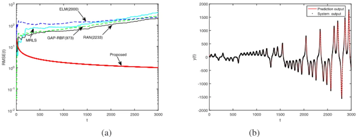
Table II and Figure 2(a) compares RMSE learning curves for different approaches respectively. Figure 2(b) plots model prediction of proposed SLSSVR approach. It is clear that the proposed SLSSVR has significantly better performance than the others. In fact, the SLSSVR is effectively the only approach here that can track well this highly nonstationary Lorenz time series.
B. UK FTSE index prediction
In this example, Istanbul stock exchange data set is con-sidered [32]. This data set includes returns of Istanbul Stock Exchange with seven other international index; SP, DAX, FTSE, NIKKEI, BOVESPA, MSCE EU, MSCI EM from Jun 5, 2009 to Feb 22, 2011. We applied the proposed SLSSVR to model one day ahead prediction for FTSE index, the daily return index of UK stock exchange. The system input is based on recent four data samples of
xt= [y(t), y(t−1), y(t−2), y(t−3)]T (32)
and system output is yt=y(t+ 1).
Table III and Figure 3(a) compare the final prediction performance and RMSE learning curves in nonstationary case for different approaches, respectively. It can be observed that compared to other methods, the proposed has the best performance, and linear MRLS is the worst, with the RMSE value of 0.6643 which is much higher than others. Note that the ELM approach with 70 and 10 nodes are only better than the MRLS. The model sizes of non-linear RAN and GAP-RBF approaches are 14 nodes and 10 nodes. In contrast the
proposed algorithm returns only 10 kernels selected from 50 full model size (average number of kernels with non-zeros parameters).
Figure 3(b) shows the FSTE time series, and it is clear that it is nonstationary. Figure 3(c) is a scatted plot of predicted output against the system output, demonstrating excellent match. Figure 3(d) illustrates the local prediction output and the system output in nonstationary time series online, and it is clearly observed that the proposed algorithm predicts well with only 10 kernels. In fact, the RMSE results may become worse by the model size increasing in nonstationary scenario. The primary reason is that the local information characteristic is more important than the global information. In this paper, the proposed algorithm add the forget factor to “forget” the previous data faster than others, hence, it focuses more attention on the new data. In general the stock index is a non-stationary time series, which is influenced by multiple external factors such as policy, season, marketplace. The example illustrates the potential of our modeling approach, which could be extended to more complicated economic model, e.g. with other leading indicators as system input variables.
V. CONCLUSIONS
In this paper, we have proposed a novel online sparse least squares support vector regression methodology based on a
sliding window of recent data set of sizeN. In order to obtain
a sparse model per time step, thel1penalty was applied in
pa-rameter estimation in the dual problem based on least squares support vector regression with forgetting factor (without bias term). An iterative algorithm has been introduced based on the Gauss-Seidel algorithm with guaranteed convergence, together
with l1-norm regularization. It is shown that a very sparse
model per time step can be obtained very efficiently.
the benchmark Lorenz time series in which their system parameters are suddenly changed. In addition the proposed algorithm has been compared for the UK FTSE index predic-tion. The proposed approach is shown to be superior to other approaches including the linear recursive least algorithm and a number of online non-linear approaches in terms of modelling performance and model size. It can be potentially utilised in time signal processing and adaptive control applications (e.g., target tracking) with nonstationary properties in practical systems, which will be our future work.
VI. ACKNOWLEDGEMENT
This work was supported by the National Natural Science Foundation of China (No.61603369), the Natural Science Foundation of Fujian Province of China (No.2018J06019), the Chunmiao Project of Haixi Institute of CAS (Program No.CMZX-2016-005).
REFERENCES
[1] W. Bartelmus, F. Chaari, R. Zimroz, M. Haddar, “Modelling of gearbox dynamics under time-varying nonstationary load for distributed fault detection and diagnosis,”European Journal of Mechanics, 29(4):637-646. 2010.
[2] L. Li, Z. Yang, B. Wang, M. Kitsuregawa, “Dynamic adaptation strategies for long-term and short-term user profile to personalize search,” InJoint, Asia-Pacific Web and, International Conference on Web-Age Information Management Conference on Advances in Data and Web Management, Springer-Verlag, pp.228-240, 2007.
[3] T. Susnjak, A. L. C. Barczak, K. A. Hawick, “Adaptive cascade of boosted ensembles for face detection in concept drift,” Neural Computing and Applications, 21(4):671-682, 2012.
[4] H. Chen, Y. Gong, X. Hong, “A new adaptive multiple modelling ap-proach for non-linear and non-stationary systems,”International Journal of Systems Science, 47(9):1-11,2014.
[5] H. Chen, Y. Gong, X. Hong, S. Chen. “A Fast Adaptive Tunable RBF Network For Nonstationary Systems,”IEEE Transactions on Cybernetics, 46(12):2683-2692, 2016.
[6] V. Vapnik,Statistical Learning Theory, Wiley, 1998.
[7] A. J. Smola, B. Sch´’olkopf, “A tutorial on support vector regression,”
Statistics and Computing, Vol 14, pp199-222, 2004.
[8] J. C. Platt, “Fast training of support vector machines using sequential minimal optimization,” in B. Sch´’olkopf, C. Burges, A. Smola, eds,
Advances in Kernel Methods: Support Vector Machines, MIT Press, Cambridge, MA, December, 1998.
[9] S. K. Shevade, S. S. Keerthi, C. Bhattacharyya, K.R.K. Murthy, “Improve-ments to the SMO algorithm for SVM regression,”IEEE Transactions on Neural Networks, 11(5):1188-1193, 2000.
[10] Y. J. Lee, W. F. Hsieh, C. M. Huang,“ε-SSVR: A Smooth Support Vector Machine forε-Insensitive Regression,”IEEE Transactions on Knowledge and Data Engineering, 17(5):678-685, 2005.
[11] W. Wang, Z. Xu, “A heuristic training for support vector regression,“
Neurocomputing, 61(1):259-275, 2004.
[12] J. Bi, K. P. Bennett, “A geometric approach to support vector regression,”
Neurocomputing, 55(1-2):79-108, 2003.
[13] S. Mukherjee, E. Osuna, F. Girosi, “Nonlinear prediction of chaotic time series using a support vector machine,” InNeural Networks Signal Processing VII, Proc. of the 1997 IEEE Signal Processing Society Workshop, Amelia Island, FL, USA, Sep 24-26, 1997.
[14] J. T. Jeng, C. C. Chuang, S. F. Su, “Support vector interval regression networks for interval regression analysis,”Fuzzy Sets and Systems, vol. 138, no. 2, pp. 283-300, Sep. 2003.
[15] J. A. K. Suykens, J. De Brabanter, L. Lukas and J. Vandewalle, “Weighted least squares support vector machines: robustness and sparse approximation,”Neurocomputing, Vol. 48, 1-4, pp85-105, 2002. [16] T. T. Chen, S. J. Lee, “A weighted LS-SVM based learning system for
time series forecasting,“Information Sciences, 299(C):99-116, 2015.
[17] W. Zhang, C. Hu, L.Jiao and R. Shang, “Forgetting-factor least square support vector machine and application on drift forecasting of gyro,”
Journal of Astronautics, 2, pp040, 2007.
[18] C. Saunders, A. Gammerman, V. Vovk, “Ridge regression learning in dual variables,” InProc of the 15th Internationa Conference on Machine Learning, ICML-98, Madison-Wisconsin, 1998
[19] C. Rasmussen, C. Williams,Gaussian Processes for Machine Learning, MIT Press, 2006.
[20] R. S. Varga,Matrix Iterative Analysis, Prentice Hall, Englewoods Cliffs and New Jersey, 2007.
[21] F. Ding, Y. Shi, and T. Chen, “A new identification algorithm for multiinput ARX systems,” inProc. IEEE Int. Conf. Mechatron. Autom.,
vol. 2, pp. 764-769, 2005
[22] F. Ding and T. Chen, “Performance analysis of multi-innovation gradient type identification methods,” Automatica, vol. 43, no. 1, pp. 1-14, Jan. 2007.
[23] F. Ding, P. Liu, and G. Liu, “Multiinnovation least-squares identification for system modeling,”IEEE Trans. Syst., Man, Cybern. Part B, Cyber-netics, vol. 40, no. 3, pp. 767-778, Jun. 2010.
[24] J. Platt, “A resource-allocating network for function interpolation,”
Neural Comput., vol. 3, no. 2, pp. 213-225, Jun. 1991.
[25] G.-B. Huang, P. Saratchandran, and N. Sundararajan, “An efficient sequential learning algorithm for growing and pruning RBF (GAP-RBF) networks,”IEEE Trans. Syst., Man, Cybern. B, Cybern.,vol. 34, no. 6,pp. 2284-2292, Dec. 2004.
[26] G.-B. Huang, P. Saratchandran, and N. Sundararajan, “A generalized growing and pruning RBF (GGAP-RBF) neural network for function approximation,”IEEE Trans. Neural Netw.,vol. 16, no. 1, pp. 57-67,Jan. 2005.
[27] G.-B. Huang, Q.-Y. Zhu, and C.-K. Siew, “Extreme learning machine: A new learning scheme of feedforward neural networks,” inProc. IEEE Int. Joint Conf. Neural Netw.,Jul. 2004, vol. 2, pp. 985-990.
[28] G.-B. Huang, Q.-Y. Zhu, and C.-K. Siew, “Extreme learning machine: Theory and applications,”Neurocomputing,vol. 70, no. 1-3, pp. 489-501, Dec. 2006.
[29] N.-Y. Liang, G.-B. Huang, P. Saratchandran, and N. Sundararajan, “A fast and accurate online sequential learning algorithm for feedforward networks,” IEEE Trans. Neural Netw., vol. 17, no. 6, pp. 1411-1423, Nov. 2006.
[30] G.-B. Huang, H. Zhou, X. Ding, and R. Zhang, “Extreme learning machine for regression and multiclass classification,” IEEE Trans. Syst., Man, Cybern. B, Cybern.,vol. 42, no. 2, pp. 513-529, Apr. 2012. [31] H. Chen, Y. Gong, X. Hong, “Online modeling with tunable RBF
network.” IEEE Transactions on Systems Man and Cybernetics Part B Cybernetics,43(3):935-947, 2012.
TABLE I
PERFORMANCE OFLORENZTIME SERIES WITH SYSTEM COEFFICIENT DRIFT;T = 40
Algorithm RMSE MAE nodes or kernels MRLS 7.8679 6.2666 NA RAN 4.6341 3.8969 208 GAP-RBF 4.0734 3.1621 86 ELM(500) 3.0163 2.1816 500 ELM(1000) 0.7113 0.4871 1000 ELM(2000) 0.1451 0.0819 2000 LSSVR 0.0330 0.00085 11 0 500 1000 1500 2000 2500 3000 t 10-3 10-2 10-1 100 101 102 RMSE(t) ELM(2000) MRLS Proposed RAN(208) GAP-RBF(86) 0 500 1000 1500 2000 2500 3000 t -20 -15 -10 -5 0 5 10 15 y(t) Prediction output System output (a) (b)
Fig. 1. Lorenz time series with system coefficient drift; (a) RMSE learning curves and (b) Model prediction and system output.
0 500 1000 1500 2000 2500 3000 t 10-2 10-1 100 101 102 103 RMSE(t) Proposed ELM(2000) MRLS GAP-RBF(973) RAN(2233) 0 500 1000 1500 2000 2500 3000 t -2000 -1500 -1000 -500 0 500 1000 1500 2000 y(t) Prediction output System output (a) (b)
Fig. 2. Lorenz Time series with time based Drift; (a) RMSE learning curves and (b) Model prediction and system output.
TABLE II
PERFORMANCE OFLORENZTIME SERIES WITHTIMEBASEDDRIFT;T= 40
Algorithm RMSE MAE nodes or kernels MRLS 387.6135 230.2607 -RAN 206.8554 134.8254 2233 GAP-RBF 266.7767 174.3732 973 ELM(500) 322.8352 207.0891 500 ELM(1000) 295.0591 192.2465 1000 ELM(2000) 237.1711 148.8609 2000 LSSVR 1.0107 0.0430 11
TABLE III
PERFORMANCE OF THEFTSETIME SERIES
Algorithm RMSE MAE nodes or kernels MRLS 0.6643 0.3601 -RAN 0.2310 0.2762 14 GAP-RBF 0.1993 0.2503 10 ELM(10) 0.5574 0.3057 10 ELM(70) 0.3145 0.1862 70 LSSVR 0.1114 0.1146 10 0 100 200 300 400 500 600 t 10-2 10-1 100 101 102 RMSE(t) MRLS ELM(10 nodes) ELM(70 nodes) RAN(14 nodes) GAP-RBF(10 nodes) Proposed 0 100 200 300 400 500 600 t -60 -40 -20 0 20 40 60 Stock Index
Real stock dataset
(a) (b) -60 -40 -20 0 20 40 60 System output -60 -40 -20 0 20 40 60 Predition output System output Prediction output 400 405 410 415 420 425 430 435 t -20 -15 -10 -5 0 5 10 15 20 25 y(t) System output Prediction output (c) (d)