ADCHEM 2006
International Symposium on Advanced Control of Chemical Processes Gramado, Brazil – April 2-5, 2006
MODELING AND IDENTIFICATION OF NONLINEAR SYSTEMS USING SISO LEM-HAMMERSTEIN AND LEM-WIENER MODEL STRUCTURES
P. Bolognese Fernandes, D. Schlipf, J. O. Trierweiler
Group of Integration, Modeling, Simulation, Control and Optimization of Processes (GIMSCOP) Department of Chemical Engineering, Federal University of Rio Grande do Sul (UFGRS)
Rua Luiz Englert, s/n CEP: 90040-040 – Porto Alegre – RS – Brazil Fax: +55 51 3316 3277, Phone: + 55 51 3316 4072
Email: [email protected], [email protected], [email protected]
Abstract: This paper applies the concept of linearization around the equilibrium manifold (LEM) already presented in the literature in order to construct model structures that can be viewed as extensions of the conventional Wiener and Hammerstein models. Instead of linear time-invariant subsystems in association with static nonlinearities, these extensions exhibit variable dynamic character and can therefore model a broader class of systems than the conventional cited approaches. Moreover, the identification strategy already used with LEM systems can be applied in order to construct such models from experiments, and the techniques destined for analysis and control of Wiener and Hammerstein systems can be applied promptly. To application of these concepts to the modeling and identification is demonstrated with a numerical example, considering a heat exchange system. Copyright © 2006 IFAC
Keywords: System Identification; Nonlinear Models; Linearization; Interpolation; Wiener Systems; Hammerstein Systems.
1. INTRODUCTION
In order to control satisfactorily a nonlinear plant, two main approaches exist: either the use of “inherent” nonlinear control techniques or the use of robust linear methods to guarantee stability and adequate performance in despite of the nonlinear effects. In the first approach, it is necessary that nonlinear dynamic models are available, what is very often not the case. This is mainly due to the cost of nonlinear modeling and/or identification, but also to the fact that universal and fail-free methods allowing for the identification of accurate nonlinear models are still missing.
In order to describe the nonlinear characteristics that are encountered in the practice, it is often adequate to
consider a given dynamic system as the composition of a linear dynamic block followed by a static nonlinearity, the so-called Wiener system. By reversing the order of the blocks, the result is the Hammerstein model. There is a plenty of literature on specific methods for identification of either Hammerstein or Wiener models, or both. A good survey on these model structures can be found in (Pearson, 1995).
Although interesting from the practical point of view, these approaches may be too simple if the description of a nonlinear dynamics is sought. Therefore, the concept of linearization around the equilibrium manifold (LEM) can be used to include such characteristic in the model representation. The advantage of the LEM systems is that they can be
constructed in a straightforward manner and result in simple, transparent model structures.
This paper is organized as follows: Section 2 reviews the concept of LEM systems already discussed in the literature, which is the basis for the two proposed model structures. Extended Hammerstein and Wiener models, in which the dynamics are dependent of the operating point, are shown in Sections 3 and Section 4, respectively. The models are then applied in Section 5 in the modeling and identification of a nonlinear system in a numerical example. Concluding remarks can be found in Section 6.
2. LEM SYSTEMS
Consider a continuous SISO nonlinear dynamic system of the form
) ( ) , ( x x r x h y u = =
(1)
where r:X×U→ ℜn is at least once continuously differentiable on X⊆ ℜn,U⊆ ℜ, and h: X → ℜ is at least once continuously differentiable. The output equation will be frequently omitted in the sequel for shortness. The equilibrium manifold of (1) is defined as the family of constant equilibrium points
(
)
{
}
) , ( , ) , ( : , , s s s s s n s s s u y u y u x h 0 x r x = = ℜ × ℜ × ℜ ∈ = Ξ.
(2)Similarly, the family of Taylor linearizations of (1) at the set of equilibrium points determined by (2) is given by ) ( ) , ( ) ( ) , ( , ,u s u s u u u u u s s s s − »¼ º «¬ ª ∂ ∂ + − »¼ º «¬ ª ∂ ∂ = x x x r x x x x r x (3)
and similarly for the output equation. Under the condition that the rank of [∂r(xs,us)/∂x] is n for all
points in the set Ξ (Wang and Rugh, 1987, Fernandes 2005), the equilibrium manifold and consequently the family of linearizations of (1) will be specified by one among the n+ 1 variables (x,u). Therefore, if this matrix is full rank, the input fully parameterizes both families of equilibrium points and linearizations. Calling the steady-state map Ω:ℜĺℜn, such that
r(Ω(u),u)=0 (that is, the function Ω gives the steady-state xs corresponding to the constant input
us), the input-parameterized linearization around the
equilibrium manifold (LEM) of (1) is defined as the system (Fernandes 2005, Fernandes and Engell, 2005). )) ( )( (u x ȍu A x= − (4)
where A(u) represents the evaluation of the Jacobian matrix [∂r(x,u)/∂x] on (Ω(u),u). Observe that the term arising from the second part of (3) is dropped by letting u=us. The output equation can be linearized
in an analogous fashion, considering the stationary
output mapping Ȍ:ℜĺℜ. The output function Ω(u) can be obtained on the basis of the family of parameterized linearizations by integration of
) ( ) ( ) ( 1 u u du u d B A ȍ − − =
.
(5)where A and B are the Jacobian matrices of
r(x,u) with respect to x and u, respectively, evaluated on the equilibrium manifold. The model (4) has to be interpreted as a (state-affine) nonlinear system that possesses the same family of equilibrium points (2) and the same linearization family (3) as the nonlinear system (1). Following the discussion in (Fernandes, 2005), the LEM system can constitute also a good approximation of (1) in transient regimes away from the equilibrium manifold, depending on the “degree” of nonlinearity of the original system. Obviously, other representations that are equivalent on the equilibrium manifold can be constructed on the basis of a single parameter, other than u. Moreover, these representations can be easily interchanged, provided that the inverses of the corresponding elements in Ω(u) and Ȍ(u) exist.
The focus on input parameterization is due to the fact that identification experiments are carried out by exciting the plant with a designed input signal. In this sense, if one assumes that the local models can be identified by perturbing the plant around isolated equilibrium points, it is natural to use the input in order to parameterize the linearization family. Additionaly, since the exact LEM system (4) involves the infinite family of linearizations and of the equilibrium points of (1), described by the matrix functions A(u) and Ω(u), in the identification context just a finite and probably small number of the members of these families are known, but one can still use approximation or interpolation methods (for example, polynomials, splines and so on) in order to “reconstruct” these functions from the available members. Therefore, an approximation to (1) can be constructed by means of a finite number of linear local models that are considered as members of its linearization family, obtained by means of a few “local” identification experiments. In order to solve the problem of constructing a state-space representation from local models obtained from input-output experiments, these can be transformed to a linear canonical normal form prior to the constructions of the approximate functions A~(u) and
) ( ~
u
ȍ (Fernandes and Engell, 2005). In the absence of the values of all steady-states, the last function can be obtained by integration of −A(u)−1B(u) (Fernandes, 2005).
3. SISO LEM-HAMMERSTEIN MODELS
The LEM concept can be used to construct a Hammerstein-like model of (1) in which the dynamics depends on the operating point instead of
the LTI dynamics encountered in the usual Hammerstein structure (see Fig. 1).
Fig. 1. LEM-Hammerstein model
A generic model with this structure can be defined in state-space form by cx b x f b x f x = + = + = y u q w ( ) ( ) ) ( (6)
where b and c are vectors of proper dimensions. A possibility of constructing a model of the form of Eq. (6) on the basis of the LEM models is to separate the static nonlinear gain function from the family of transfer functions (Pearson and Pottmann, 2000), that is, 1 ) ( ) ( ) ( 1 ) ( ) ( ) ( ) ; ( 1 1 1 1 1 1 1 1 + δ α + + δ α + δ α + δ β + + δ β ⋅ δ = δ − − − − s s s s s k s G n n n n n n (7)
where δ is a scalar parameterizing the set of equilibrium points/linearizations (us in this case). The
resulting LEM-Hammerstein system is of the form
x y u q w w w c ȍ x A x = = − =~( )( ~( )), ( ) (8) with δ δ =
³
( )d ) ( uk u q (9)such that the overall family of transfer functions correspond to that of (6). The LEM system (8) can be constructed with realizations of the parameterized transfer function of Eq. (7) in a suitable chosen coordinate basis, as for example a canonical or normal form. Obviously, Eq. (8) depends on the new input w, but an equivalent state- or output-parameterization can be easily constructed, as discussed above. These are nevertheless dynamically “worse” than the input-parameterized version (Fernandes, Engell and Trierweiler, 2004). This model can be obtained from experiments using the LEM approach as follows:
• identification of local linear models around some isolated operating points;
• transformation of the family of local models into a family of unit-gain linearizations;
• integration of k(us)= −C(us)A(us)−1B(us) in order
to obtain q(u);
• interpolation of A and B in some suitable canonical form and integration of in
) ( ) (w 1Bw A − − order to generate ȍ~(w).
Alternatively, since the “local” gain is the derivative of the stationary mapping with respect to u at a given
operating point, q can be directly obtained by means of observations of the stationary output. This procedure can also be used iteratively, that is, values ofys can be used to refine the interpolation of k and
vice-versa.
4. SISO LEM-WIENER MODELS
In parallel to the Hammerstein-type structure considered above, it is also possible to define an “extended” Wiener model by replacing the linear block with an element exhibiting variable dynamics (Fig. 2).
Fig. 2. LEM-Wiener model
Note that this model is not obtained by simply reversing the order of the blocks in Fig. 1, since the function h is a scalar valued function of n arguments whereas q is a n-valued function of one argument (that is, a collection of scalar functions).
This model can be defined in the state-space in the same fashion as in Eq. (6). Nevertheless, due to the nonlinear dependence of h on x, the input-parameterized LEM model would exhibit a direct feedthrough characteristic, what is not desirable for simulation (Fernandes, 2005). This problem can be avoided by constructing an output-parameterized LEM system, provided that the adequate conditions hold (Wang and Rugh, 1987); in the SISO case, for example, this implies that there is no change of the sign of the stationary gain. In any case, the LEM-Wiener model is given by
) ( )) ( )( ( ) ( 1 1 1 2 1 x x h y x u x g f x x x x x n n n n n = φ − + = = = − (10) where
¦
¦
= − = − + = − = n j j j n j j j n x x b x h x x a f 2 1 1 1 2 1 1 ) ( ) ( ) ( ) ( x x (11)where the functions ai(x1), bj(x1), j,i = 0,…, n – 1,
j 0, correspond to the coefficients of the parameterized transfer function
) ( ) ( ) ( 1 ) ( ) ; ( 0 1 1 1 1 ⋅ δ δ + + δ + + + δ = δ − − − − n n n n n n g a s a s s b s G (12)
q
(
u
)
G
u
(
t
)
w
(
t
)
y
(
t
)
Static
Nonlinearity
Dynamics
( )
(
t
)
(
t
)
(
t
)
Static
Nonlinearity
Non-linear
G
h
(x)
u
(
t
)
x(
t
)
y
(
t
)
Non-linear
Dynamics
Static
Nonlinearity
( )
(
t
)
(
t
)
(
t
)
Static
Nonlinearity
where δ is a scalar parameterizing the set of equilibrium points/linearizations (x1,s in this case),
and a0(x1)= −gn(x1)⋅dφ(x1)/dx1. The “advantage” of
this form for identification is that all involved functions are scalar and can be therefore identified by means of the variation of one single parameter. Moreover, since the steady-states of this representation are of the form x1,s=ys, xj,s= 0,
j = 2,…, n, these functions can be obtained by means of local linear models parameterized by the output. Another advantage of the LEM-Wiener model structure is that it can be further extended by including a second-order term in the output equation, in order to improve the accuracy of the model away from the equilibrium manifold, that is,
) ( ) ( ) ( 2 1 1 1 ĭ x x = +
¦
+ = − n j j j x x b x h (13)where Φ(x) is such that Φ(xs) = 0 and
[∂ΦΦ(x)/∂x]xs = 01×n. In particular, one possibility for
Φ(x) is
(
( ))
(
( ))
)
(x x ȍx1 TH x ȍ x1
ĭ = − − (14)
where the n×n matrix H has to be adjusted from experiments, and Ω(x1) = [ x1 0 … 0 ]T. The advantage is that H does not affect the dynamics of (10) and consequently avoids several problems. Moreover, since the output depends linearly on H, it can be adjusted by means of computationally simple methods (least-squares, for example).
5. NUMERICAL EXAMPLE: HEAT EXCHANGE SYSTEM
The model structures presented in the previous sections will be tested in the modeling and simulation of the heat exchange system (Duraiski, 2001) depicted in Fig. 3. Fci, Tci Fi, Ti Fhi, Thi Fc, Tc F, T Fh, Th Vh V h VV c V Vc Uh V hVV c Uc
Fig. 3. Heat exchange system
This system is constituted by an insulated tank divided in three separate chambers that are allowed to transfer heat but not mass. The central chamber is in contact with both hot (h) and cold (c) chambers, but these are in contact just with the central one. The volumes of the chambers Vh,V and Vc, are constant,
and all chambers are well-mixed. Water is fed to and removed from each chamber separately. Under these
assumptions, the system can be described by means of the following differential equations:
(
)
(
)
(
)
( ) ( ) ) ( ) ( T T Cp V A U T T Cp V A U V T T F dt dT T T Cp V A U V T T F dt dT T T Cp V A U V T T F dt dT c c c h h h i i c c c c c c ci ci c h h h h h h hi hi h − ρ ⋅ ⋅ ⋅ + − ρ ⋅ ⋅ ⋅ + − ⋅ = − ρ ⋅ ⋅ ⋅ − − ⋅ = − ρ ⋅ ⋅ ⋅ − − ⋅ = (15)where Th, Tc and T are the temperatures of each
chamber, Cp and ρ are the specific heat and specific
mass of water (considered to be independent of the temperature), Uh (Uc) and Ah (Ac) are respectively the
overall heat exchange coefficient and heat exchange area between the corresponding chambers. A more detailed description of this system can be found in (Duraiski, 2001). In this example, the input variable is considered to be the feed flowrate of hot water,
Fh,i, which has constant temperature Th,i. The output
is the temperature of the central chamber, T. The values considered for the physical parameters and other inflows can be found in the Appendix. The variation of the dynamic character is obvious from the analysis of Fig. 4 and Fig. 5.
5.1 Constructing an approximated model in LEM, LEM-Hammerstein and LEM-Wiener forms
The original LEM, LEM-Hammerstein and LEM-Wiener models described in the previous sections can be constructed analytically on the basis of the model (15). In the first case, we have a system in the form of Eq. (4) with
» » » ¼ º « « « ¬ ª + + + ⋅ + = » » » ¼ º « « « ¬ ª − − − − = 2 . 376 2 . 469 2 . 376 2 . 469 2 . 376 4 . 470 254 . 1 272 . 1 1 ) ( 322 . 0 0797 . 0 239 . 0 0797 . 0 0797 . 0 0 239 . 0 0 239 . 0 0033 . 0 ) ( u u u u u u u ȍ A (16)
and y=x3. For the LEM-Hammerstein model, it is first necessary to convert the matrices above to a normal form in order that the individual transfer functions from w to y in Fig. 1 have unit gain. The system is of the form:
» » ¼ º « « ¬ ª = » » ¼ º « « ¬ ª − − − − − − − = − w w w u u u u 54 . 12 0 ) ( ~ 974 . 7 0 100 002 . 0 101 . 0 2 . 56 33 . 0 35 . 1 105 . 0 0 100 0 10 ) ( ~ 2 ȍ A (17) where u has to be substituted by q−1(w) for implementation, with 25 . 1 27 . 1 2 . 376 2 . 469 ) ( + + = = u u u q w
.
(18)
The LEM-Wiener model (10)-(11) can be constructed similarly, giving
2 1 1 1 1 1 1 3 1 1 2 1 1 5 . 12 ) ( 0304 0 2 11 000418 0 125 0 8 71 0000645 0 0238 . 0 ) ( ) 0304 0 2 11 ( ) 1 14 0383 0 ( 507 0 ) 0304 0 2 11 ( ) 27 1 00342 0 ( 507 0 ) ( x x h x . - . x . - . . x . - x g x x . - . . x . -. x x . - . . x . -. f n n + = − = φ = + − + − = x x
.
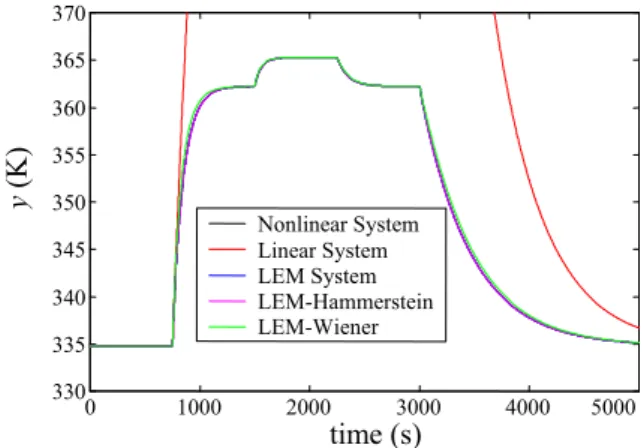
(19)The systems described above were simulated in Matlab with respect to the input function shown in Fig. 4; the responses are plotted in Fig. 5. The response of the linearized model at the operating point determined by us=1 is also shown for
comparison. Excepting this system, the other curves are practically indistinguishable.
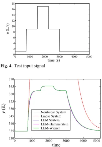
Fig. 4. Test input signal
Fig. 5. Responses of the several systems to the signal in Fig. 3
5.2 Constructing the approximated models with identified local models
Approximated versions of the models derived in the previous section can be constructed with local models obtained either from linearizations or from identification experiments; only the last approach is exemplified here. The following procedure was adopted: three linear local models corresponding to the operating points defined by us,1= 1 L/s (ys,1 = 334.76 K), us,2= 8 L/s (ys,2= 361.46 K), us,3= 15 L/s
(ys,3 = 364.78 K) were identified by means of “local experiments”, that is, with identification signals of small amplitude around these operating points. No special methodology was employed to select the number or the location of these points; they were simply distributed over a desired range of the manipulated input. For each operating point, an identification signal uid of the form depicted in Fig. 6
was designed. The switching period σ of the signal was determined as t63/20, where t63 is the time needed from the step response to reach 63% of its steady-state value, what was obtained previously for each point by means of a step test with the nonlinear model (positive step of 0.2 L/s in u). The amplitude of the identification signal was fixed to 30% of us,i.
An input sequence of the form us,i−uid was
employed with validation purposes.
Fig. 6. Identification input signal
The response of the nonlinear model (15) was simulated in Matlab for the identification signal uid.
In order to simulate the effect of measurement error, a white-noise, Gaussian sequence with zero mean and standard deviation of 0.01 K was added to the output. A typical plot of the noisy output measurement is given in Fig. 7. The simulated signals were sampled with a convenient sample period in order to be used with the identification algorithms.
Fig. 7. Noisy and filtered output
Since an accurate representation of the local linearizations is necessary, the following procedure was adopted. First, a set of two runs was performed with uid for each operating point and the average of
the corresponding outputs yid was taken as the
0 σ 2σ 3σ 4σ 5σ us,i− ∆i us,i us,i+∆i time (s) u (L/s) 0 1000 2000 3000 4000 5000 0 2 4 6 8 10 12 14 16 18 time (s) u (L/s) 0 1000 2000 3000 4000 5000 330 335 340 345 350 355 360 365 370 time y (K ) Nonlinear System Linear System LEM System LEM-Hammerstein LEM-Wiener 0 50 100 150 334.7 334.8 334.9 335 335.1 time (s) y (K)
identification data; this has the objective of reducing the effect of noise. Second, the data was filtered by means of a least-squares smoothing cubic spline (Matlab function spap2). The best parameter set of the spline function was determined iteratively in function of the results of the identification procedure achieved in the subsequent step.
The linear local models in discrete form were identified through the combined use of subspace (Matlab functions n4sid/subid) and state-space prediction error methods (Matlab function pem). The subspace methods gave the initial estimates for the prediction error method and were also used for determining the order of the state-space models. As already suggested in the literature (Fernandes, 2005), the authors found that a good local identification is generally achieved when the order of the model is clearly evidenced by the singular value test provided by the subspace routines. Moreover, a frequent indication of excessive model order and poor identification by these methods is the generation of unstable poles, complex zeros, etc. The identification procedure was as follows: first, the filtered data was used in the subspace methods; the model order was selected and the estimates were passed to the pem
routine. This result was then simulated and validated against the identification and validation data. If necessary, the parameters of the smoothing spline function were changed, the data was filtered again and the local models identified once more; this procedure was repeated until a good result was found.
The local models identified in this manner were used in the construction of the model structures presented in the sections 2, 3 and 4. The LEM and LEM-Hammerstein models were constructed with local models in observability form. The last one differs from the analytical case because the linear transformation to normal form depends on the relative degree which is not a “robust” quantity to be obtained from experiments. In all cases, proper spline or rational interpolation of the necessary functions was performed (the results are omitted due to the space limitations). The responses of the three structures with identified local models for the input signal in Fig. 4 are shown in Fig 8; the agreement with the nonlinear model is quite good. The most significant difference with respect to the analytical case refers to the Wiener model, due to the identification/interpolation of the bi parameters that
appear in the output function.
6. CONCLUSIONS
This paper presented new model structures based on the concept of linearization around the equilibrium manifold (LEM). These models extend the conventional Hammerstein and Wiener systems, in the sense that they allow for the inclusion of variable dynamics. These representations can be constructed on the basis of local models, which can be obtained
for example by identification. A numerical example (bilinear system) showed that these structures are almost equivalent if the models are obtained analytically, but the effect of the errors in the estimated parameter can affect differently the distinct model classes.
Fig. 8. Responses of the several systems constructed on the basis of identified local models
APPENDIX Parameter values used in the example:
ρ = 1000 kg/m3,Cp= 4180 J/kg/K, V=Vc=Vh= 0.3 m3 Uh . Ah= 300.000 J/K/s, Uc . Ac= 100.000 J/K/s Fci= 0 m3/s, Tci= 280 K, Fi= 0.001 m3/s,Ti= 300 K Thi= 370 K AKNOWLEDGEMENTS
The authors thank FINEP and PETROBRAS for the financial support. The first and second authors thank respectively the German Academic Exchange Service (DAAD) and the Landesstiftung Baden-Württemberg.
REFERENCES
Duraiski, R. G (2001). Controle Preditivo Não-Linear Utilizando Linearização ao Longo da Trajetória. Masters’ Thesis, Federal University of Rio Grande do Sul, Brazil (in Portuguese).
Bolognese Fernandes, P., S. Engell, J. O. Trierweiler (2004). A new approach to the local models networks technique. Proceedings of the Brazilian Congress of Engenharia Química, COBEQ04, Curitiba, Brazil. Bolognese Fernandes, P. (2005). The input-parameterized
linearization around the equilibrium manifold approach to modeling and identification. Phd Thesis, University of Dortmund (to be published).
Bolognese Fernandes, P., S. Engell (2005). Continuous Nonlinear SISO System Identification using Parameterized Linearization Families. Proc. of the XVI IFAC World Congress,Prague,Tchech Republic. Pearson, R. K (1995). Gray-box identification of
block-oriented nonlinear models. Journal of Process Control,10, 301-315.
Pearson, R. K. and M. Pottmann (2000). Gray-box identification of block-oriented nonlinear models. Journal of Process Control,10, 301-315.
Wang, J. and J. W. Rugh (1987). Parameterized Linear Systems and Linearization Families for Nonlinear Systems. IEEE Transactions on Circuits and Systems,
34, 650-657. 0 1000 2000 3000 4000 5000 330 335 340 345 350 355 360 365 370 time (s) y (K ) Nonlinear System Linear System LEM System LEM-Hammerstein LEM-Wiener