University of Central Florida University of Central Florida
STARS
STARS
Electronic Theses and Dissertations, 2004-2019 2013
Accelerated Life Model With Various Types Of Censored Data
Accelerated Life Model With Various Types Of Censored Data
Kathryn Pridemore University of Central Florida
Part of the Mathematics Commons
Find similar works at: https://stars.library.ucf.edu/etd University of Central Florida Libraries http://library.ucf.edu
This Doctoral Dissertation (Open Access) is brought to you for free and open access by STARS. It has been accepted for inclusion in Electronic Theses and Dissertations, 2004-2019 by an authorized administrator of STARS. For more information, please contact [email protected].
STARS Citation STARS Citation
Pridemore, Kathryn, "Accelerated Life Model With Various Types Of Censored Data" (2013). Electronic Theses and Dissertations, 2004-2019. 2678.
ACCELERATED LIFE MODEL WITH VARIOUS TYPES OF
CENSORED DATA
by
KATIE PRIDEMORE
B.S. Mathematics, Stetson University, 2003 M.S. Mathematics, University of Central Florida, 2005
A dissertation submitted in partial fulfillment of the requirements for the degree of Doctor of Philosophy
in the Department of Mathematics in the College of Sciences at the University of Central Florida
Orlando, Florida
Summer Term 2013
Major Professor: Marianna Pensky
c
ABSTRACT
The Accelerated Life Model is one of the most commonly used tools in the analysis of survival data which are frequently encountered in medical research and reliability studies. In these types of studies we often deal with complicated data sets for which we cannot observe the complete data set in practical situations due to censoring. Such difficulties are particularly apparent by the fact that there is little work in statistical literature on the Accelerated Life Model for complicated types of censored data sets, such as doubly censored data, interval censored data, and partly interval censored data.
In this work, we use the Weighted Empirical Likelihood approach (Ren, 2001) [33] to
construct tests, confidence intervals, and goodness-of-fit tests for the Accelerated Life Model in a unified way for various types of censored data. We also provide algorithms for imple-mentation and present relevant simulation results.
I began working on this problem with Dr. Jian-Jian Ren. Upon Dr. Ren’s departure from the University of Central Florida I completed this dissertation under the supervision of Dr. Marianna Pensky.
TABLE OF CONTENTS
LIST OF FIGURES . . . viii
LIST OF TABLES . . . ix
CHAPTER 1 INTRODUCTION . . . 1
1.1 Introduction . . . 2
1.2 Accelerated Life Model . . . 4
1.2.1 Two-Sample Accelerated Life Model . . . 4
1.2.2 General Accelerated Life Model . . . 6
1.2.3 Review of Recent Work . . . 9
1.3 Censored Data . . . 12
1.3.1 Right Censored Data . . . 13
1.3.2 Doubly Censored Data . . . 14
1.3.3 Interval Censored Data . . . 16
1.4 Likelihood . . . 21
1.4.1 Parametric Likelihood . . . 21
1.4.2 Empirical Likelihood . . . 23
1.4.3 Weighted Empirical Likelihood . . . 26
1.5 Centered Gaussian Processes . . . 30
1.6 Summary of Main Results . . . 30
CHAPTER 2 ESTIMATION AND GOODNESS OF FIT . . . 33
2.1 Weighted Empirical Likelihood for Accelerated Life Model . . . 33
2.2 Treatment Distribution Estimator . . . 36
2.3 Goodness of Fit for Accelerated Life Model . . . 42
CHAPTER 3 ESTIMATION AND TESTS ON SCALE PARAMETER . . . 47
3.1 Naive Estimator . . . 47
3.1.1 Hypothesis Tests based on Normal Approximation . . . 49
3.2 Rank-Based Estimator . . . 52
3.2.1 Hypothesis Tests . . . 53
3.2.2 Confidence Intervals . . . 54
3.2.3 Computability . . . 55
3.3 Weighted Empirical Likelihood Ratio Tests and Confidence Intervals . . . . 60
3.3.1 Hypothesis Tests . . . 61
3.3.2 Confidence Intervals . . . 70
CHAPTER 4 ESTIMATION AND TESTS ON TREATMENT MEAN . . . 83
4.1 Point Estimators . . . 83
4.2 Normal-Approximation Based Tests and Confidence Intervals . . . 85
4.2.1 Hypothesis Tests . . . 86
4.2.2 Confidence Intervals . . . 88
4.3 Weighted Empirical Likelihood Ratio Tests and Confidence Intervals . . . . 88
4.3.2 Confidence Intervals . . . 106
4.3.3 Computation of Confidence Intervals . . . 111
CHAPTER 5 SIMULATION STUDIES. . . 117
5.1 Review of Bootstrap Percentile Confidence Intervals . . . 117
5.2 Point and Interval Estimators of a Scale Parameter . . . 118
5.2.1 Point Estimators for the Scale Parameter . . . 119
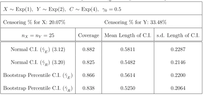
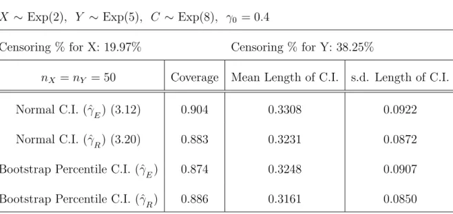
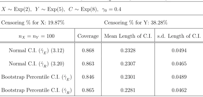
5.2.2 Interval Estimators for the Scale Parameter . . . 121
5.3 Point and Interval Estimators of the Treatment Mean . . . 124
5.3.1 Point Estimators for the Treatment Mean . . . 125
5.3.2 Interval Estimators for the Treatment Mean . . . 126
5.4 Simulations for the Treatment Distribution Function . . . 130
5.5 Summary of Simulation Results . . . 134
CHAPTER 6 CONCLUDING REMARKS . . . 135
LIST OF FIGURES
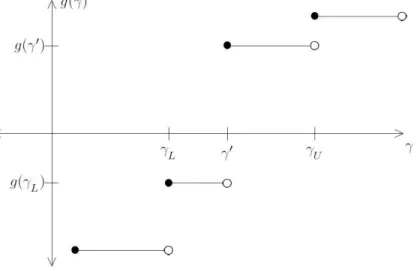
3.1 Scenarios for g(λ): |g(γL)|<|g(γ0)| . . . 57
3.2 Scenarios for g(λ): |g(γL)|>|g(γ0)| . . . 57
3.3 Scenarios for g(λ): |g(γL)|=|g(γ0)| . . . 58
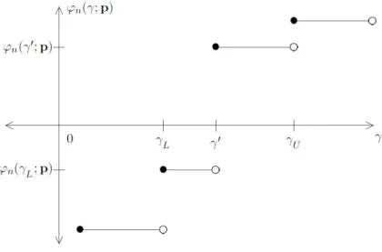
3.4 Scenarios for ϕ(γ;p) for fixed p∈E1∪E2 . . . 74
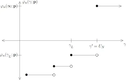
3.5 Scenarios for ϕ(γ;p) for fixed p∈E3: ϕ(U1;p)<0ϕ(UN−1;p)>0 . . . 75
3.6 Scenarios for ϕ(γ;p) for fixed p∈E3: ϕ(U1;p)>0 . . . 75
LIST OF TABLES
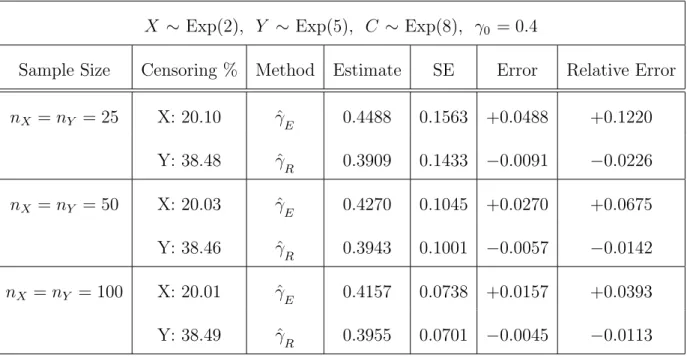
5.1 Point Estimators for the scale parameter γ0 . . . 120
5.2 Point Estimators for the scale parameter γ0 . . . 120
5.3 90% C.I. for the scale parameter γ0 with right censored exponential data . . . . 121
5.4 90% C.I. for the scale parameter γ0 with right censored exponential data . . . . 122
5.5 90% C.I. for the scale parameter γ0 with right censored exponential data . . . . 122
5.6 90% C.I. for the scale parameter γ0 with right censored exponential data . . . . 123
5.7 90% C.I. for the scale parameter γ0 with right censored exponential data . . . . 123
5.8 90% C.I. for the scale parameter γ0 with right censored exponential data . . . . 124
5.9 Point Estimators for the treatment mean µX . . . 125
5.10 Point Estimators for the treatment mean µX . . . 126
5.11 90% C.I. for the treatment meanµ0 with right censored exponential data. . . . 127
5.13 90% C.I. for the treatment meanµ0 with right censored exponential data . . . 128
5.14 90% C.I. for the treatment meanµ0 with right censored exponential data . . . 129
5.15 90% C.I. for the treatment meanµ0 with right censored exponential data . . . 129
5.16 90% C.I. for the treatment meanµ0 with right censored exponential data . . . 130
5.17 Estimators for Treatment Distribution: d1 =kGˆ−FXk d2 =kFˆn−FXk . . . 133
CHAPTER 1
INTRODUCTION
TheAccelerated Life Modelis one of the most commonly used tools in the analysis of survival data. Due to the nature of survival data, we often encounter data sets which are subject to censoring, i.e., we cannot observe the complete data set in practical situations. Until now, there has been little work in statistical literature on the Accelerated Life Model for complicated types of censored data sets, such as doubly censored data, interval censored
data, and partly interval censored data. In this research, we use the Weighted Empirical
Likelihood approach (Ren, 2001) [33] to construct tests, confidence intervals, and goodness-of-fit tests for the Accelerated Life Model in a unified way for various types of censored data.
This chapter is organized as follows. Section 1.1 briefly introduces some basic concepts and notations in survival analysis. Section 1.2 introduces the Accelerated Life Model and re-views some relevant recent works. Section 1.3 describes various types of censored data with examples, and reviews some relevant asymptotic results on the nonparametric maximum likelihood distribution estimators. Section 1.4 reviews the techniques of Parametric Like-lihood, Empirical Likelihood (Owen, 1988)[31], and Weighted Empirical Likelihood (Ren, 2001)[33]. Finally, Section 1.6 summarizes the main results of this dissertation, and outlines the organization of the rest of this dissertation.
1.1 Introduction
Survival analysis is an area of statistical research which is concerned with the failure time of subjects. An example of this in medical research is a treatment study where a new drug or treatment is being tested. Researchers may want to determine the effects of the new treatment on survival time for patients with diseases such as diabetes, AIDS, cancer, etc.
While there may be many different explanatory variables, survival analysis primarily deals with a univariate lifetime variable, which is often referred to as failure time. To determine failure time precisely, we need a clearly defined time origin, a way of measuring time, and an explicit definition of the meaning of failure. In medical research, the time origin is usually defined as the time at which a patient enters a clinical trial, time is measured in days or months, and failure is defined as the time when a disease relapses or the time when a patient dies from the disease of interest.
One challenge in the analysis of survival data is that in practical situations, we often are unable to observe the failure time of an individual due to censoring. Such a challenge can be quite difficult to handle mathematically, which is why there has been so little work done in the statistical literature on the Accelerated Life Model with complicated types of censored data, such as doubly censored, interval censored, and partly interval censored data. But it is well known that these complicated types of censored data are encountered in important clinical trials in medical research; see Section 1.3 for descriptions of various types of censored data
and real data examples. Thus, it is important for us to develop new statistical procedures to handle these types of censored data.
As follows, we introduce some commonly used definitions and notations in survival
anal-ysis. Let T denote the lifetime random variable, which is continuous and nonnegative. And
letfT(t) andFT(t) denote the density function and distribution function ofT, respectively. Definition 1.1. The survival function of T is defined by
¯
FT(t) = P{T ≥t} = 1−FT(t). (1.1)
Definition 1.2. The hazard function of T is defined by
hT(t) = lim
∆→0+
P{t≤T < t+ ∆ | T ≥t}
∆ . (1.2)
Note that the hazard function is the instantaneous rate of mortality at timetgivenT ≥t. Also, note that Definition 1.2 implies that the hazard function can be expressed in terms of the density function and distribution function of T as below:
hT(t) = lim ∆→0+ P{t ≤T < t+ ∆ | T ≥t} ∆ = lim∆→0+ P{t≤T < t+ ∆} P{T ≥t} ·∆ = lim ∆→0+ FT(t+ ∆)−FT(t) ¯ FT(t)·∆ = F 0 T(t) ¯ FT(t) = f¯T(t) FT(t) . (1.3)
The hazard function hT(t) in (1.2) plays a key role in the Cox Proportional Hazards
Model (Cox, 1972) [8], which is one of the most commonly used models in survival analysis. However, the model assumptions of the Cox Proportional Hazards Model do not hold in some practical situations. Hence, the Accelerated Life Model is a commonly used alternative model in survival analysis. In the next section, we describe the Accelerated Life Model and discuss its relation to the Cox Proportional Hazards Model.
1.2 Accelerated Life Model
In this section, we describe the Accelerated Life Model (ALM). Specifically,
Subsection 1.2.1 discusses the Two-Sample Accelerated Life Model; Subsection 1.2.2 discusses the general case of the Accelerated Life Model and its relationship with the Cox Proportional Hazards model; and Subsection 1.2.3 briefly reviews some recent relevant works on the Accelerated Life Model.
1.2.1 Two-Sample Accelerated Life Model
The basic underlying assumption for the Accelerated Life Model is that the covariate vector
z acts multiplicatively on the failure times. The following summarizes the relevant topics from Section 5.1 of Cox and Oakes (1984). [9]
Consider the simple case where we have a single indicator variable z such that z = 0
corresponds to the control group, andz = 1 corresponds to the treatment group. In survival analysis, this could mean a study which assesses the effectiveness of a new medical treatment that is anticipated to increase the survival time of individuals in, say, a cancer study. The data from the treatment group z = 1 and the control group z = 0 are the following lifetime random samples, respectively:
Treatment z = 1 : X1, . . . , Xn1 i.i.d. ∼ FX, Control z = 0 : Y1, . . . , Yn0 i.i.d. ∼ FY. (1.4)
The assumption of the Accelerated Life Model is that lifetime random variables X and Y
are proportional to each other, which is denoted by
Y = X
γ0, (1.5)
where γ0 is an unknown positive scale parameter, and model (1.5) is referred to as the
Two-Sample Accelerated Life Model.
From model assumption (1.5), the following relationships among the distribution
func-tion, density funcfunc-tion, and hazard function of the random variables X and Y are implied:
FY(t) = P{Y ≤t} = P X γ0 ≤t = P{X ≤γ0t} = FX(γ0t), fY(t) = FY0 (t) = [FX(γ0t)]0 = FX0 (γ0t)γ0 = fX(γ0t)γ0, hY(t) = fY(t) ¯ FY(t) = fX(γ0t)γ0 ¯ FX(γ0t) = hX(γ0t)γ0. (1.6)
In the Two-Sample Accelerated Life Model (1.5), we also make the following observations. If γ0 > 1, then the failure time of X is greater than the failure time of Y. In terms of the clinical study, this indicates that the treatment is effective. On the other hand, if 0< γ0 ≤1, then the failure time ofX is not greater than the failure time of Y, which indicates that the treatment is not effective.
In practice, the scale parameterγ0 in (1.5) is unknown. For statistical inferences, we use the available data to estimate γ0. To determine if the treatment is effective, the following hypothesis test may be considered:
H0 : 0< γ0 ≤1 (treatment not effective)
H1 : γ0 >1 (treatment effective).
Also, point estimators and interval estimators for γ0 based on the available data may be used to assess the effectiveness of the treatments.
1.2.2 General Accelerated Life Model
In the general case, we may be interested in the effects of several different variables or covariates on the failure time. For these cases, we consider, more generally, a covariate vector zof explanatory variables, and the general Accelerated Life Model is given by
T = T0
ψ(z), (1.8)
where T0 corresponds to the baseline lifetime random variable with z =0, and ψ(z) ≥0 is
a function of the explanatory variables z satisfying ψ(0) = 1. Below is an example on the general Accelerated Life Model (1.8).
Example 1. Consider a new treatment for lung cancer with z = (z1, z2, z3), where
z1 = gender; z2 = treatment; and z3 = [change in size of tumor]. In model (1.8), we haveT
as survival time from lung cancer treatment.
From model assumption (1.8), the following relationships among the distribution func-tion, density funcfunc-tion, and hazard function of the lifetime random variables T and T0 are
implied. Let F0 denote the distribution function of T0, then we have F(t;z) = P{T ≤t} = P T0 ψ(z) ≤t = P{T0 ≤tψ(z)} = F0(tψ(z)), f(t;z) = F0(t;z) = F00(tψ(z))ψ(z) = f0(tψ(z))ψ(z), h(t;z) = f¯(t;z) F(t;z) = f0(tψ(z))ψ(z) ¯ F0(tψ(z)) = h0(tψ(z))ψ(z). (1.9)
Moreover, taking the natural logarithm of both sides of (1.8) yields
logT = logT0−logψ(z) = µ0−logψ(z) +, (1.10)
where µ0 is the mean of logT0, and is a random variable with mean 0 whose distribution
does not depend on z.
In some cases, a parametric form for ψ(·) may be needed, say, in the form of ψ(z;β) by introducing a parameter β. Since we require ψ(z) =ψ(z;β)≥0 and ψ(0;β) =1 in (1.10), a natural choice is
ψ(z;β) =eβTz. (1.11)
With this choice, Accelerated Life Model (1.8) or (1.10) is written as
logT =µ0−βTz+, (1.12)
which is the log linear model with parameter β, and the usual linear model technique may
used to study this model.
Two-Sample ALM vs. General ALM. In (1.11), we have ψ(0, β) = 1 and
ψ(1, β) = eβ ≡γ
0. Thus, a special case of (1.8) with function (1.11) for z = 0, 1 gives:
T = T0 ψ(0;β) =T0, T = T0 ψ(1;β) = T0 γ0, (1.13)
which coincides with the Two-Sample Accelerated Life Model (1.5). In the situation with a limited number of distinct values ofz, it is unnecessary to specify a parametric form forψ(z) such as (1.11), and with limited information, if any, about the underlying distribution, the choice of (1.11) may not even be reasonable. In cases where we have only a few treatment levels, we may use pairwise studies, i.e., the Two-Sample Accelerated Life Model (1.5), to compare the effects of different treatments. For these reasons, we focus on the Two-Sample Accelerated Life Model (1.5) throughout the rest of this dissertation.
Relation to Proportional Hazards Model. The Accelerated Life Model and the Cox Proportional Hazards model are the two main models used in survival analysis. The
Cox Proportional Hazards Model (Cox, 1972) [8] is given by
h(t;z) =h0(t)eβ
>z
, (1.14)
where h(t;z) is the conditional hazard function of T given Z =z, and h0(t) is an arbitrary
baseline (control group) hazard function. It has been shown that the Accelerated Life Model and Cox Proportional Hazards Model coincide if and only if the failure time follows a Weibull distribution (Cox and Oakes, 1984; page 71-72)[9]. When there is no evidence that the survival time follows a Weibull distribution or when the Cox Model assumption does not hold for the available data, it is vital to develop estimation and testing procedures for the Accelerated Life Model which is an important alternative model to the Cox Model in survival analysis.
Model Checking. The Accelerated Life Model is applicable when different levels of stress or different treatments are applied to subjects and each different level of stress or
treatment is in turn believed to increase or decrease the failure time of the subjects. As mentioned previously, we can study the effects of new medical treatments that are antici-pated to increase the survival time of individuals in the study. Since the distributions of logT
in (1.12) differ only by a translation for different values ofz, the variance of logT should be constant. A simple analysis where we calculate the mean and standard deviation at different treatment levels can help to determine if the model is adequate. In treatment levels where severe censoring is present, the mean and standard deviation may be over or underestimated. In these cases, we need to explore different methods to deal with the censoring issue, and it is always desirable to develop goodness-of-fit tests for assessment of the validity of the model assumptions. In the context of this research, goodness-of-fit tests for the Two-Sample Accelerated Life Model (1.5) with various types of censored data are important. If the data set does not fit the model assumption, then any statistical conclusion under model assump-tion (1.5) is not reliable. To our best knowledge, up to now there has been no work done on goodness-of-fit tests for the Two-Sample Accelerated Life Model (1.5) for complicated types of censored data such as doubly censored, interval censored, and partly interval censored data, which are described in Section 1.3.
1.2.3 Review of Recent Work
Rank-based monotone estimating functions are developed for the ALM with right censored observations in Jin, Lin, Wei and Ying (2003).[21] Using a resampling technique, which
does not involve nonparametric density estimation or numerical derivatives, they estimate the limiting covariance matrices. These estimators, which are given by the roots of non-monotone estimating equations based on the familiar weighted log-rank statistics, are shown to be consistent and asymptotically normal. These estimators can be obtained by linear programming, and two examples are provided to show that the proposed methods perform well in practical settings.
Using semiparametric transformation models, Cai and Cheng (2004) [5] analyze doubly censored data with additional assumptions on the right and left censoring variables. In their paper, inference procedures for the regression parameters are given, and the asymptotic distributions are studied.
Chen, Shen and Ying (2005) [7] also consider right censored data and propose a rank estimation procedure based on stratifying a Gehan-type extension of the Wilcoxon-Mann-Whitney estimating function. The resulting estimate is shown to be consistent and asymp-totically normal. It is shown that the stratification poses little loss of information. These techniques can be done with linear programming.
Using the empirical likelihood method, Zhou (2005) [46] derives a test based on the rank estimators of the regression coefficient for the Accelerated Life Model with right censored data. Simulations and examples show that the chi-squared approximation to the distribution of the log empirical likelihood ratio performs well and has some advantages over the existing methods.
Odell, Anderson, and D’Agostino (1992) [30] study a Weibull-based accelerated failure time model with left and interval censored data. This approach assumes a parametric model. Maximum likelihood estimators (MLEs) are compared with Midpoint estimators (MDEs) and simulation studies indicate many instances where the MLE is superior to the MDE.
Betensky, Rabinowitz, and Tsiatis (2001) [4] study the accelerated failure time model with interval censored data using estimating equations computed using examination times from the same individual treated as if they had been obtained from different individuals. This approach does not involve computing the nonparametric maximum likelihood estimate of the distribution function. Simulation results are provided.
Komarek, Lesaffre, and Hilton (2005) [24] estimate parameters of an accelerated failure time model using a semiparametric approach they developed. In this approach, they use a P-spline smoothing technique which directly provides predictive survival distributions for fixed values of covariates with the presence of left, right, and interval censored data. Applications of this approach are provided as well.
Tian and Cai (2006) [41] use a novel approach to make inferences about the parameters in the accelerated failure time model for current status and interval censored data through an estimator constructed by inverting a Wald-type test for testing a null proportional hazards model. In addition, a Markov chain Monte Carlo based resampling method is proposed to obtain, simultaneously, the point estimator and a consistent estimator of its variance-covariance matrix. Extensive numerical studies are provided.
Komarek and Lesaffre (2008) [25] explore the relationship of covariates to the time to caries of permanent first molars. An accelerated failure time model with random effects is suggested, taking into account that the observations are clustered. These methods involve analyzing multivariate doubly and interval-censored data. Model parameters are estimated using a Bayesian approach with Markov chain Monte Carlo methodology.
To our best knowledge, up to now, the Accelerated Life Model has not been considered in literature, in a unified way, for all of the types of censored data considered in this dissertation.
1.3 Censored Data
Let
X1, X2, . . . , Xn (1.15)
be a random sample from an unknown distribution function F0. In practice, we often do
not actually observe this sample due to censoring. In the following subsections, we describe various types of censored data along with some real data examples, and summarize the asymptotic results on the nonparametric maximum likelihood estimator ˆFn forF0.
1.3.1 Right Censored Data
The observed data for the random sample (1.15) areOi = (Vi, δi), 1≤i≤n, with
Vi = Xi if Xi ≤Ci, δi = 1 Ci if Xi > Ci, δi = 0, (1.16)
whereCi is theright censoring variableand is independent ofXi. This type of censored data
has been extensively studied in statistical literature in the past few decades.
Data Example 1. Heart Transplant Data. In Miller and Halpern (1982), [28], a right censored data set is presented, and a brief description of the this data set is as follows. The Stanford heart transplantation program began in October 1967. By February 1980, 184 patients had received transplants. In this example, Xi is the survival time after a heart
transplant. Of these 184 patients, 71 were still alive at the end of the study; thus for each of these patients, Xi occurs at some point after the study, resulting in 71 right censored
observations.
NPMLE and Asymptotic Properties: The likelihood function forF0 based on right
censored data (1.16) is given in Kaplan and Meier (1958). [22]. Thenonparametric maximum
likelihood estimator(NPMLE) ˆFn forF0 is the function that maximizes this likelihood
func-tion. For right censored data, the product-limit estimator of Kaplan and Meier (1958) [22] is
the unique NPMLE for F0. For right censored data, Wellner (1982) [43] showed the
asymp-totic efficiency of the NPMLE ˆFn. In Gill (1983) [14], it is shown that
√
converges to a centered Gaussian process under certain conditions. Also, it has been shown by Stute and Wang (1993) [40] that ||Fˆn−F0||
a.s.
−−→0, as n→ ∞.
1.3.2 Doubly Censored Data
The observed data for the random sample (1.15) areOi = (Vi, δi), 1≤i≤n, with
Vi = Xi if Di < Xi ≤Ci, δi = 1 Ci if Xi > Ci, δi = 2 Di if Xi ≤Di, δi = 3, (1.17)
whereCi is aright censoring variable,Di is aleft censoring variable, and (Ci, Di) is
indepen-dent ofXi withP{Di < Ci}= 1.As mentioned previously in Subsection 1.2.3, the results in
Cai and Cheng (2004) [5] only apply to a special case of above doubly censored data (1.17). Specifically, Cai and Cheng (2004) [5] impose the restrictive assumption that the left and right censoring variables are always known, but in (1.17) the censoring variables are not al-ways observed and the left and right censoring variablesCi andDi are never observed at the
same time. Thus, up to now, there have been no works on the Accelerated Life Model (1.5) for doubly censored data (1.17).
Data Example 2. African Infant Precocity. A classic example of doubly censored data,
discussed in Turnbull (1974) [42], comes from Leiderman et al. (1973) [26], and a brief
description of this data set is as follows. In Leidermanet al. (1973) [26], a study was done in a community in Kenya to establish norms for infant development as compared to the known
standards in the United States and the United Kingdom. The data set contains information on 65 children born between July 1 and December 31, 1969. The infants were tested at approximately 2-month intervals, beginning in January, 1970, to see when they learned a certain task. In this example, Xi is the age of an infant when he/she can first perform the
certain task. Some infants were able to perform the task at the first test; thus for these infants,Xi occurs at some point before the first test, resulting in left censored observations.
On the other hand, some infants were never able to perform the task during the study; thus for these infants, Xi occurs at some point after the final test, resulting in right censored
observations. For the remaining infants, the first time that they performed the task was observed, resulting in uncensored observations.
Data Example 3. Effectiveness of Screening Mammograms. In Ren and Peer (2000), [37] a doubly censored data set is studied, and a brief description of this data set is as follows. The study is based on the serial screening mammograms obtained in Njmegen, The Nether-lands, 1981-1990. There were 289 patients in the study. In this example, Xi is the age at
which the tumor can be detected for theith patient when biennial mammographic screening
is the only detection method. Of these patients, 45 had tumors observed at their first
screen-ing mammogram; thus for each of these patients, Xi occurs at some point before the study
began, resulting in 45 left censored observations. On the other hand, 132 of the patients never had a tumor observed; thus for these patients, Xi occurs at some point after the study
ended, resulting in 132 right censored observations. For the remaining 112 patients, a tumor was detected during the serial screening mammogram, i.e., the tumor was observed at one
mammogram at time t= Xi, but was not observed in the previous mammogram. Thus for
each of these patients, Xi was actually observed, resulting in 112 uncensored observations.
NPMLE and Asymptotic Properties: The likelihood function forF0based on doubly
censored data (1.17) is given in Mykland and Ren (1996). [29] The NPMLE ˆF forF0based on
the data (1.17) is the distribution function that maximizes the likelihood function. Mykland and Ren (1996) [29] give necessary and sufficient conditions for a self-consistent estimator
for F0 to be the NPMLE. In Turnbull (1974), [42] an iterative procedure was proposed to
obtain an estimate for the survival function when the data is grouped. For the general case,
Mykland and Ren (1996) [29] give an algorithm to compute the NPMLE ˆFn. It has been
shown by Chang and Yang (1987) [6] and Gu and Zhang (1993) [17] that||Fˆn−F0||
a.s.
−−→0,as
n→ ∞. It is also shown in Gu and Zhang (1993) [17] that for doubly censored data (1.17), that √n( ˆFn−F0) weakly converges to a centered Gaussian process under certain regularity
conditions.
1.3.3 Interval Censored Data
Case 1: The observed data for the random sample (1.15) areOi = (Ci, δi), 1≤i≤n, with
Case 2: The observed data for the random sample (1.15) areOi = (Ci, Di, δi), 1≤i≤n, with δi = 1 if Di < Xi ≤Ci 2 if Xi > Ci, 3 if Xi ≤Di, (1.19)
where Ci and Di are independent of Xi and satisfy P{Di < Ci}= 1.
Data Example 4. HIV Data. The following interval censored case 2 data (1.19) were en-countered in AIDS reserach; see De Gruttola and Lagakos (1989),[10] and see Ren (2003) [34] for a detailed discussion, while a brief description is as follows.
In De Gruttola and Lagakos (1989), [10] an interval censored data set on
X ={time of HIV infection}
from AIDS research was presented. Since 1978, 262 people with Type A and B haemophilia have been treated at Hˆopital Kremlin Bicˆetre and Hˆopital Cœur des Yvelines in France. For each individual, the only information available on X is X ∈ [XL, XR], while it is assigned XL= 1 if the individual was found to be infected with HIV on his/her first test for infection.
Along with the retrospective tests for evidence of HIV infection, observations XL and XR
were determined by the time at which the blood samples were stored. In this data set, time
is measured in 6-month intervals, with X = 1 denoting July 1978, and one of the interests
Kim, De Gruttola and Lagakos (1993) [23] gave the updated version of this data set for 104 individuals in the heavily treated group, i.e., patients who received at least 1000 µg/kg of blood factor for at least one year between 1982 and 1985. This data set always satisfies
XL< XR, and it is associated with interval censored case 2 data (1.19) in the following way:
1< XL < XR<∞ ⇐⇒ δ= 1, D=XL, C =XR
1< XL< XR=∞ ⇐⇒ δ= 2, D=XL, C =∞
1 =XL< XR<∞ ⇐⇒ δ= 3, D= 1, C =XR.
Note that due to the way in which XL and XR were determined, we may assume that
[XL, XR] is independent of X, because the available blood samples were stored purely from
haemophilia treatment which had nothing to do with HIV infection Thus, this is a real data example for interval censored case 2 data (1.19).
NPMLE and Asymptotic Properties: The likelihood functions for F0 based on
interval censored data (1.18) and (1.19) are given in Groeneboom and Wellner (1992), [15] respectively. The NPMLE ˆFn forF0 in each case is the distribution function that maximizes
the respective likelihood function. It is shown in Groeneboom and Wellner (1992) [15] that we have ||Fˆn−F0||
a.s.
−−→0,as n → ∞. For interval censored case 1 data (1.18), we have
n1/3[ ˆFn(t0)−F0(t0)]
D
−→C0Z, asn→ ∞ (1.20)
where C0 is a constant and Z =argmin(W(T) + t2) with W as the two sided Brownian
motion starting from 0. For interval censored case 2 data (1.19), Wellner (1995) [44] and Groeneboom (1996) [16] showed that (1.20) holds under certain regularity conditions. But
the general convergence rate for ˆFn with interval censored case 2 data (1.19) is not known
up to now.
1.3.4 Partly Interval Censored Data
Case 1: The observed data for the random sample (1.15) are
Oi = Xi if 1≤i≤k0 (Ci, δi), if k0 + 1≤i≤n, (1.21)
where δi =I{Xi ≤Ci}and Ci is independent of Xi.
General Case: The observed data for the random sample (1.15) are
Oi = Xi if 1≤i≤k0 (C,δi), if k0+ 1 ≤i≤n, (1.22)
where for N potential examination times C1 < · · · < CN, letting C0 = 0 and CN+1 = ∞,
we have C = (C1, . . . , CN) and δi = (δ (1) i , . . . , δ (N+1) i ) with δ (j) i = 1, if Cj−1 < Xi ≤ Cj; 0,
elsewhere. This means that for intervals (0, C1],(C1, C2], . . . ,(CN,∞), we know which one
of them Xi falls into.
Data Example 5. Framingham Heart Disease Study. Odellet al. (1992) [30] discuss a partly interval censored data set originally found in Feinleib et al. (1975), [13] and a brief description of the data set is as follows. The original Framingham Heart Study began in 1949 to determine the genetic effects of risk factors. In the follow up study on the children of
the original patients we have 2,568 female children. Each of these individuals was observed at the Framingham Heart Study facilities in Boston, Massachusetts at three different exam times to determine the first occurrence of subcategory angina pectoris (AP) in coronary heart disease. In this example,Xi is the time that theith patient acquires AP, and C1 < C2 < C3
denote the three exam times. Also,C0 = 0 andC4 =∞. For 8 of the patients, Xi is actually
observed. None of the 2,568 patients had acquired AP by the first exam; thus Xi did not
occur in the interval [0, C1) for any patients in the study. Of the 2,568 patients, 16 patients
had not acquired AP by the second exam; thus for these patients, Xi occurs in the interval
[C1, C2). Of the 2,568 patients, 13 patients had not acquired AP by the second exam, but
had acquired AP by the third exam; thus for these patients,Xioccurs in the interval [C2, C3).
The remaining 2,531 had not acquired AP by the third exam; thus for these patients, Xi
occurs in the interval [C3,∞), resulting in 2,531 right censored observations.
NPMLE and Asymptotic Properties: The likelihood functions for F0 based on the
partly interval censored data (1.21) and (1.22) are given in Huang (1999), [18] respectively. The NPMLE ˆFn for F0 for each case is the distribution function maximizing the respective
likelihood function. Huang (1999) [18] showed that for partly interval censored data (1.21) and (1.22), ||Fˆn −F0||
a.s.
−−→ 0, as n → ∞, and that √n( ˆFn −F0) weakly converges to a
1.4 Likelihood
In this section, we briefly review the likelihood methods. Specifically, Subsection 1.4.1 re-views parametric likelihood; Subsection 1.4.2 rere-views empirical likelihood (Owen,1988); [31]; and Subsection 1.4.3 discusses weighted empirical likelihood (Ren, 2001). [33]
1.4.1 Parametric Likelihood
Consider a random sampleX1, X2, . . . , Xn from a distribution with density functionf(x;θ),
where θ ∈ Rq is an unknown parameter. Heuristically, the likelihood function is the
prob-ability that we observe what we observed. This translates into the following parametric
likelihood function L(θ|X) for parameter θ:
L(θ |X) =P{Observe what we observed}=
n Y
i=1
f(Xi |θ), (1.23)
where X= (X1, X2, . . . , Xn). If we can maximize L(θ |X) with respect to θ over the entire
parameter space Θ, then the value ˆθ, at which L(θ | X) attains its maximum, is called the
maximum likelihood estimator (MLE) for θ. Consider the following hypothesis test:
H0 :θ=θ0 vs. H1 :θ6=θ0. (1.24)
Then, the likelihood ratio test statistic is given by:
R(X;θ) = supH0L(η|X) supL(η;X) = supη=θ0 L(η|X) L(ˆθ |X) = L(θ0 |X) L(ˆθ |X), (1.25)
and the rejection region for (1.24) is:
{X|R(X;θ)≤c} (1.26)
for some predetermined constant 0 < c < 1. With the level of significance 0 < α < 1, we can determine c in the following way:
α=P{Type I error} = P{reject H0 |H0} = P{R(X;θ)≤c|θ =θ0}
=P{R(X;θ0)≤c} = P{−2 logR(X;θ0)≥ −2 logc} ≈ P{χ21 ≥ −2 logc},
(1.27)
because Wilks (1938) [45] showed that the limiting distribution of −2 logR(X;θ0) is a
chi-squared distribution.
The acceptance region for (1.24) is
{X|R(X;θ)≥c}. (1.28)
Let
λ(η) = L(η|X)
L(ˆθ|X). (1.29)
Then, a (1−α)100% confidence interval for θ =θ0 is given by:
C(X) ={η |λ(η)≥c}. (1.30)
When using parametric likelihood methods based on (1.23), we assume that the data come from a known distribution up to an unknown parameter. The main problem with this method is that in practical situations, we may not know anything about the underlying distribution. Assuming an incorrect underlying distribution can lead to incorrect statistical conclusions. This is especially a concern in survival analysis where sample sizes are generally small or
moderate, thus usually there is no sufficient information to justify the parametric assumption on the underlying distribution. Hence, a nonparametric approach is not only desirable, but is essential in survival analysis. In the next subsection, we outline the nonparametric likelihood method, called the empirical likelihood method, which provides flexibility through the use of a likelihood function that requires no parametric assumption on the underlying distribution.
1.4.2 Empirical Likelihood
Consider a random sample X1, X2, . . . Xn from an unknown distribution function F0. In
Owen (1988) [31], the empirical likelihood function or nonparametric likelihood function is given as: L(F) = n Y i=1 [F(Xi)−F(Xi−)], (1.31)
where F is any distribution function. It is shown that the distribution function that maxi-mizes (1.31) over all distribution functions F is theempirical distribution function, denoted by Fn(x) = 1 n n X i=1 I{Xi ≤x}, −∞< x < ∞. (1.32)
Next, we review the empirical likelihood method which is analogous to the parametric like-lihood method described in the previous section.
Assume that a parameter θF0 of F0 can be expressed as θF0 = T(F0), where T(·) is a statistical functional. Analogous to (1.24), we consider the following hypothesis test:
Then, the empirical likelihood ratio test statistic for (1.33) analogous to (1.25) is given by: R(X|F0) = supF∈H0L(F) supFL(F) = sup T(F)=θ0 L(F) L(Fn) , (1.34)
where Fn is given in (1.32) and the rejection region analogous to (1.26) is:
{X|R(X|F0)≤c} (1.35)
for some predetermined constant 0 < c < 1. With the level of significance 0 < α < 1, analogous to (1.27), we can determine c in the following way:
α = P{Type I error} = P{reject H0 | H0} = P{R(X|F0)≤c | T(F0) =θ0}
= P{R0 ≤c} = P{−2 logR0 ≥ −2 logc} ≈ P{χ21 ≥ −2 logc},
(1.36)
where underH0 in (1.33)
R0 =R(X|F0), when T(F0) = θ0, (1.37)
because Owen (1988) [31] showed that, usually,−2 logR0 has a limiting chi-square
distribu-tion under the null hypothesis.
The acceptance region for (1.33) analogous to (1.28) is:
{X|R(X|F0)≥c}. (1.38)
Similar to (1.25) and (1.29), let
λ(F) = L(F)
L(Fn)
. (1.39)
It can be shown that whenT(F) is continuous, a (1−α)100% confidence region for θF0 =θ0 analogous to (1.29)−(1.30) is given by C(X) = θ sup T(F)=θλ(F)≥c = {θ =T(F)|λ(F)≥c}. (1.40)
In the special case where the parameter of interest is the mean of F0, i.e.,
θF0 =T(F0) =
Z
xdF0(x), (1.41)
Owen (1988) [31] showed that the confidence region (1.40) is an interval. Specifically, Owen (1988) [31] established the following theorem.
Theorem 1 (Owen, 1988) Assume F0 is non-degenerate with
R |x|3 dF 0 < ∞. For 0< c <1, and for θ0 = R xdF0(x), we have in (1.40) C(X) = [XL,n, XU,n], (1.42) where XL,n = infF R
x dF and XU,n = supF
R
x dF, and we have
lim
n→∞P(XL,n≤θ0 ≤XU,n) = limn→∞P(−2 logR0 ≤ −2 logc) = P(χ
2
1 ≤ −2 logc), (1.43) where χ2
1 is a random variable with a chi-squared distribution with 1 degree of freedom.
Generally, the empirical likelihood method approach is preferred over the parametric ap-proach in areas such as survival analysis, where, as mentioned earlier, information is limited and we have no sufficient evidence to assume a parametric form for the underlying distri-bution. Another desirable property is that empirical likelihood based confidence intervals have been shown to have good coverage levels when compared to parametric approaches Owen (2001) [32]. Much work has been done using the methods of empirical likelihood. In particular, the NPMLE ˆFn for each type of censored data mentioned in Section 1.3 was
obtained through writing out the empirical likelihood function and maximizing it. For each
type of censored data, the asymptotic properties of the NPMLE ˆFn have been studied and
summarized in Section 1.3. However, one drawback of the empirical likelihood method is that usually it is difficult to incorporate a model assumption into the formulation of the likelihood function along with censored data. Recently, Ren (2001) [33] developed a new
nonparametric method for censored data, called weighted empirical likelihood, which was
successfully used to solve several difficult statistical inference problems with different types of censored data mentioned in Section 1.3. Based on these results, we use the weighted empirical likelihood method for the problem of Two Sample Accelerated Life Model (1.5) described in Sections 1.2−1.3. In the next subsection, we outline and discuss the weighted empirical likelihood method.
1.4.3 Weighted Empirical Likelihood
In Ren (2001) [33], theweighted empirical likelihood functionis given in a simple form that is applicable to various types of censored data in a unified form. This simple form is convenient and more easily to be used for incorporating the model assumptions into the formulation of the likelihood function for censored data. Next, we describe the weighted empirical likelihood function and its applications.
As explained in Ren (2008a) [35], the weighted empirical likelihood method can be un-derstood as follows. As in equation (1.15) from Section 1.3, we consider a random sample
X1, . . . , Xn (1.44)
from an unknown distribution function F0. Recall from Section 1.3, in practice we often do
not observe the complete sample (1.44), instead we observe various types of censored data denoted by:
O1, . . . ,On, (1.45)
which is the observed censored sample for sample (1.44) and the data are possibly one of the types of censored data mentioned in Section 1.3; i.e., the Oi’s in (1.45) could be right
censored (1.16), doubly censored (1.17), interval censored Case 1 or Case 2 (1.18)−(1.19), or partly interval censored (1.21)−(1.22), etc. As reviewed in Section 1.3, the NPMLE ˆFn for F0 has been studied for censored data (1.16)−(1.22), and it is shown that from the observed
censored data (1.45), there exist m distinct points
W1 < W2 < . . . < Wm, (1.46)
along with ˆpj >0,1≤j ≤m such that the NPMLE ˆFn can be expressed as:
ˆ Fn(x) = m X i=1 ˆ piI{Wi ≤x}, (1.47)
for right censored data (Kaplan and Meier, 1958), [22] doubly censored data (Mykland and Ren, 1996), [29] interval censored data Case 1 and Case 2 (Groenboom and Wellner, 1992), [15] and partly interval censored data (Huang, 1999). [18] Specifically, for right
cen-sored data (1.16), the Wi’s are the noncensored observations and m is the number of
un-censored observations (Kaplan and Meier, 1958). [22] For the more complicated types of censored data (1.17)−(1.22) discussed in Section 1.3, theWi’s and ˆpi’s are obtained through
computing the NPMLE ˆFn. Since, as reviewed in Section 1.3, the NPMLE ˆFnis shown to be
a strong uniform consistent estimator for the underlying distributionF0 under certain
regu-larity conditions for the types of censored data aforementioned, we expect a random sample
X1∗, . . . , Xn∗ taken from ˆFn to behave asymptotically the same as random sample (1.44). Let
Fn∗ denote the empirical distribution function (1.32) of the random sampleX1∗, . . . , Xn∗, then
we have ˆFn≈Fn∗, in turn, we have n Y i=1 P{X =Xi} ≈ n Y i=1 P{X∗ =Xi∗} = m Y j=1 P{X∗ =Wj} n[Fn∗(Wj)−Fn∗(Wj−)] ≈ m Y j=1 P{X∗ =Wj} n[ ˆFn(Wj)−Fˆn(Wj−)] = m Y j=1 P{X∗ =Wj} npˆj . (1.48)
Hence, the weighted empirical likelihood function for F0 is given by
ˆ L(F) = m Y i=1 [F(Wi)−F(Wi−)]npˆi, (1.49)
whereF is any distribution function and ˆFn maximizes ˆL(F). Thus, the weighted empirical
likelihood function ˆL(F) may viewed as the asymptotic version of the empirical likelihood function L(F) in (1.31) for censored data (Ren, 2008a). [35]
Note that when there is no censoring, it is shown (Ren, 2001) [33] that the weighted empir-ical likelihood function (1.49) coincides with the empirempir-ical likelihood function (1.31) given in
Owen (1988) .[31] Also, from the formulation of (1.49), the censoring mechanism is reflected in ˆL(F) via the probability mass of the NPMLE ˆFn for F0. Since the simple form of (1.49)
depends only on the Wi’s and ˆpi’s obtained from the NPMLE ˆFn, the weighted empirical
likelihood method is easily applicable in a unified way to all of the types of censored data discussed in Section 1.3. In particular, once theWi’s and ˆpi’s are computed from the NPMLE
ˆ
Fn with the specific type of censored data, the routines for computing weighted empirical
likelihood based confidence intervals, test statistics, etc., are the same for the different types of censored data; thus weighted empirical likelihood simplifies the likelihood based com-putational problems for statistical inference problems with various types of censored data. Another advantage of the weighted empirical likelihood method based on (1.49) is that the theoretical and asymptotic results often can be obtained in a unified way via the statistical functional of the NPMLE ˆFn for different types of censored data. Moreover, the simple form
of weighted empirical likelihood function (1.49) also makes it easier to incorporate model assumptions into the formulation of the likelihood function for complicated types of cen-sored data, such as doubly cencen-sored data (1.17), interval cencen-sored Case 1 or Case 2 data (1.18)−(1.19), and partly interval censored data (1.21)−(1.22). For these complicated types of censored data, the resulting empirical likelihood function is usually very complicated and mathematically intractable.
It has been shown that the weighted empirical likelihood method can be used to solve difficult statistical inference problems with the various types of censored data mentioned above. For instance, in her recent work, Ren (2008a) [35] uses the weighted empirical
likeli-hood method to solve problems involving two sample semi-parametric models with various types of censored data, and Ren (2008b) [36] uses the weighted empirical likelihood method to construct smoothed weighted empirical likelihood ratio confidence intervals for quantiles with censored data. Based on the success of these recent works, since the problem of Two-Sample Accelerated Life Model (1.5) with complicated types of censored data described in Section 1.2, though very difficult on its own, is slightly related to the problems considered in Ren (2008a), [35] we apply the weighted empirical likelihood method to this problem in this research. It is through this weighted empirical likelihood method that we are able to provide solutions to the very difficult problems considered in this dissertation.
1.5 Centered Gaussian Processes
A Gaussian Process [39]Gis a specific type of stochastic process such that the joint density function of any subset of the random variables is itself a multivariate Gaussian random variable. When each of these random variables have mean zero, we call this a centered Gaussian Process.
1.6 Summary of Main Results
In this research, we use the Weighted Empirical Likelihood approach to study the Accelerated Life Model with all of the types of censored data mentioned in Section 1.3. We outline
and compare inferences on the the scale parameter and the treatment using both Normal-Based Approximation and the weighted empirical likelihood approach. In particular, we obtain point estimates, hypothesis tests, and construct confidence intervals for both the scale parameter and the treatment mean. We also develop goodness-of-fit tests and provide simulation results to illustrate the effectiveness of our inferences.
This dissertation is organized as follows: Chapter 1 gives an introduction to the model and methods being utilized.
Chapter 2 introduces estimation for the Accelerated Life Model and discusses goodness of fit. In particular, in Section 2.2 we construct a Treatment Distribution Estimator for FX in
(1.4), we establish asymptotic properties for this estimator in Proposition 2.2 and establish rates of convergence for the estimator in Theorem 2.3 and Theorem 2.4 for right censored data (1.16), doubly censored data (1.17), and partly interval censored data (1.21)−(1.22). At the end of Section 2.3 we provide an approach for computing the p-value for a goodness of fit test statistic for right censored data (1.16), doubly censored data (1.17), and partly interval censored data (1.21)−(1.22).
Chapter 3 discusses estimation of the scale parameter in the Accelerated Life Model (1.5). In particular, in Section 3.1 we construct a naive estimator for γ0 in (1.5), establish asymptotic properties for this estimator in Theorem 3.1 and construct normal based tests and confidence intervals for γ0 based on this estimator. In Section 3.2 we discuss a rank based estimator and construct normal based tests and confidence intervals for γ0 based on this estimator. We also provide an algorithm at the end of Section 3.2 for computing the rank
based estimator in practice which is applicable to all of the complicated types of censored data discussed in this dissertation. In Section 3.3 we discuss Weighted Empirical Likelihood Ratio based confidence intervals for γ0 based on the rank based estimator.
Chapter 4 discusses estimation for the mean µX of the treatment group in (1.4). In
particular, we construct point estimators for µX in Section 4.1. We construct normal based
tests and confidence intervals for µX based on these point estimators in Section 4.2 and
provide algorithms for computing these confidence intervals. In Section 4.3 we construct
Weighted Empirical Likelihood Ratio based confidence intervals for µX based on the rank
based point estimator and provide algorithms for computing these intervals in practice. Chapter 5 discusses the bootstrap method and provides simulation results on the work described above.
Finally, Chapter 6 summarizes the research that has been done and provides direction for further development of the ideas in this dissertation.
CHAPTER 2
ESTIMATION AND GOODNESS OF FIT
In this chapter, we study the estimation problem for the treatment distribution function
FX in (1.5) and goodness-of-fit tests for the Two-Sample Accelerated Life Model (1.5). The
methods developed in this chapter are applicable in a unified way to those different types of censored data described in Section 1.3. The organization of this chapter is as follows. Section 2.1 derives the weighted empirical likelihood function for (γ0, FX) under the
Two-Sample Accelerated Life Model (1.5). Section 2.2 obtains an estimator for the treatment distribution function FX in (1.5). Section 2.3 constructs goodness-of-fit tests for the
Two-Sample Accelerated Life Model.
2.1 Weighted Empirical Likelihood for Accelerated Life Model
Consider the Two-Sample Accelerated Life Model (1.5), and consider that the two samples in (1.4) are censored data, denoted by:
OX1 , . . . ,OXn
1 is the observed sample for treatment sample X1, . . . , Xn1
OY1, . . . ,OYn0 is the observed sample for control sample Y1, . . . , Yn0,
(2.1)
where these two observed samples are independent, and theOXi ’s orOYi ’s are possibly one of the types of censored data in Section 1.3, i.e., right censored data (1.16), doubly censored data (1.17), interval censored data Case 1 and Case 2 (1.18)−(1.19), or partly interval censored data (1.21)−(1.22). Note that it is not necessary for the two samples to be subject to the
same type of censoring; for instance, the data from the treatment group could be doubly censored and the data from the control group could be right censored.
Let ˆGand ˆH be the NPMLE forFX and FY in (1.4) based on observed first and second
censored data (2.1), respectively. As reviewed in Section 1.4.3, we know that there exist distinct points W1X <· · ·< WmX1 and W1Y <· · ·< WmY0 as in (1.46) along with ˆpX
i >0 and
ˆ
pY
j >0 such that ˆGand ˆH can be expressed as
ˆ G(x) = m1 X i=1 ˆ pX i I{W X i ≤x} and Hˆ(x) = m0 X j=1 ˆ pY j I{W Y j ≤x}, (2.2)
respectively, for various types of censored data aforementioned. Note that ˆG and ˆH in
(2.2) are not necessarily proper distribution functions. For this dissertation, we will adjust both ˆG and ˆH to proper distribution functions by setting ˆG= 1 and ˆH = 1 at the largest observations of the corresponding observed data sets in (2.1). Note that this adjustment implies that in (2.2) we have
m1 X i=1 ˆ pX i = 1 and m0 X j=1 ˆ pY j = 1, (2.3)
and that this kind of adjustment of the NPMLE is a generally adopted convention for censored data (Efron, 1967; Miller, 1976).[11] [27]
To derive the weighted empirical likelihood function for (γ0, FX) in Two-Sample
Ac-celerated Life Model (1.5) based on observed two-sample censored data (2.1), we apply weighted empirical likelihood function (1.49) as follows. First, via ˆG and ˆH in (2.2), we apply weighted empirical likelihood function (1.49) to the two observed censored samples in (2.1), respectively. Since the two observed samples in (2.1) are independent, the weighted
empirical likelihood function based on the combined two samples in (2.1) is the product of the two weighted empirical likelihood functions. Thus, from the model assumption on the Two-Sample Accelerated Life Model (1.5)−(1.6) and from assumptions (2.2)−(2.3) for the NPMLE ˆG and ˆH, we can write this weighted empirical likelihood function as follows:
Qm1 i=1[FX(WiX)−FX(WiX−)] n1pˆXi Qm0 j=1[FY(WjY)−FY(WjY−)] n0pˆYj (1.6) = Qm1 i=1[FX(W X i )−FX(WiX−)] n1pˆX i Qm0 j=1 γ0[FX(γ0WjY)−FX(γ0WjY−)] n0pˆYj = γn0 Pm0 j=1pˆYj 0 Qm1 i=1[FX(W X i )−FX(WiX−)] n1pˆXi Qm0 j=1[FX(γ0W Y j )−FX(γ0WjY−)] n0pˆYj (2.3) = γn0 0 Qm1 i=1[FX(WiX)−FX(WiX−)] n1pˆXi Qm0 j=1[FX(γ0WjY)−FX(γ0WjY−)] n0pˆYj .
Hence, the weighted empirical likelihood function for (γ0, FX) in Two-Sample Accelerated
Life Model (1.5) based on observed data (2.1) is given by
L(γ, F) = γn0 m1 Y i=1 [F(WiX)−F(WiX−)]n1pˆXi m0 Y j=1 [F(γWjY)−F(γWjY−)]n0pˆYj , (2.4)
where F is any distribution function.
To simplify (2.4) for computational purpose, we introduce the following notations:
Wγ = (W1γ, . . . , Wmγ) = (W1X, . . . , WmX 1, γW Y 1 , . . . , γW Y m0), (w1, . . . , wm) = (ρ1pˆX1 , . . . , ρ1pˆmX1, ρ0pˆY1, . . . , ρ0pˆYm0), (2.5)
wherem=m0+m1,n =n0+n1,ρ1 =n1/n, andρ0 =n0/n. From (2.5), weighted empirical
likelihood function (2.4) can be rewritten as
L(γ, F) = γn0 m Y i=1 pnwi i , (2.6)
where γ is any positive real number, and F is given by
F(x) =
m X
i=1
Hence, the weighted empirical likelihood based MLE (ˆγ,Fˆn) for (γ0, FX) is the solution that
maximizesL(γ, F) in (2.6).
2.2 Treatment Distribution Estimator
In this section, based on weighted empirical likelihood function (2.6) we derive an estimator for the treatment distributionFX in Two-Sample Accelerated Life Model (1.5) with observed
two-sample censored data (2.1), and we establish some asymptotic properties of this esti-mator for FX. Note that the weighted empirical likelihood based MLE (WELMLE) (ˆγ,Fˆn)
for (γ0, FX) is rather difficult to obtain, which requires additional restrictions and will be
discussed later in Chapter 3. Here, we consider a simpler approach to obtain an estimator for FX. The idea of this approach is that first, for a fixed γ >0, we maximize L(γ, F) over F, then we replace γ with a consistent estimator for γ0.
For a fixed γ > 0, to maximize L(γ, F) in (2.6) over all F given by (2.7), we need to solve the following optimization problem:
Maximize L(γ, F) = γn0 m Y i=1 pnwi i , subject to: 0≤pi ≤1, 1≤i≤m; m X i=1 pi = 1. (2.8)
Note that if one of the pi’s above is 0, then L(γ, F) = 0. Also, note that if one of the pi’s is
1, then constraint Pm
optimization problem (2.8) is equivalent to Maximize L(γ, F) = γn0 m Y i=1 pnwi i , subject to: 0< pi <1, 1≤i≤m; m X i=1 pi = 1. (2.9)
To solve optimization problem (2.9), we note that for all 1 ≤i≤m, we have
logL(γ, F) = n0logγ+n
m X
i=1
wilogpi. (2.10)
Thus, to find a candidate for the solution using the Lagrange Multipliers, we denote
H(p, λ) =n m X i=1 wilogpi+λ 1− m X i=1 pi , (2.11)
then, we have for 1≤i≤m,
0 = ∂H
∂pi = nwi
pi −λ ⇒ pi =nwi/λ. (2.12)
From (2.12) and constraintPm
i=1pi = 1 in (2.9), we have 1 = m X i=1 pi = m X i=1 nwi λ , (2.13)
which, along with (2.3) and (2.5), implies that
λ = m X i=1 nwi =n "m 1 X i=1 wi+ m X i=m1+1 wi # =n " ρ1 m1 X i=1 ˆ pX i +ρ0 m0 X j=1 ˆ pY j # =n[ρ1+ρ0] =n[(n1+n0)/n] =n1 +n0 =n. (2.14)
Thus, from (2.12) and (2.14) a candidate for the solution of (2.9) is given by
ˆ
p= (w1, . . . , wm). (2.15)
The following lemma shows that this candidate is the unique solution for (2.9).
Proof We prove that ˆp= (ˆp1, . . . ,pˆm), given by (2.15), is the unique solution to (2.9) by
verifying the Karush-Kuhn-Tucker (KKT) conditions in Theorem 4.3.8 of Bazarra, Sherali,
and Shetty (1993; page 164) [1] as follows. From (2.11), let
h(p) = n m X i=1 wilogpi (2.16) and let A = ( p 0< pi <1, 1≤i≤m; m X i=1 pi = 1 ) . (2.17)
The Hessian matrix (Bazarra, Sherali, and Shetty, 1993; page 90) [1] ofh(p) given in (2.16), exists on the set A and is given by
∂2h(p) ∂pi∂pj = −nwi p2 i if i=j 0 if i6=j. =⇒ Hh = diag ( −nw1 p2 1 , . . . ,−nwm p2 m ) . (2.18)
Since Hh is a diagonal matrix with diagonal elements −nwp2i
i
< 0, 1 ≤ i ≤ m, for p ∈ A,
Hh is negative definite on A. Note that A is a convex set because for any p, q ∈ A and
r=λp+ (1−λ)qwith any λ∈(0,1) we have
0< ri =λpi+ (1−λ)qi < λ+ (1−λ) = 1, 1≤i≤m; m X i=1 ri =λ m X i=1 pi + (1−λ) m X i=1 qi =λ+ (1−λ) = 1. (2.19)
Thus, functionh(p) is strictly concave onAby Theorem 3.3.8 of Bazarra, Sherali, and Shetty (1993; page 92 and page 79). [1] To verify the conditions in Theorem 4.3.8 of Bazarra, Sherali, and Shetty (1993; page 164), [1] note that Xp ={p | 0< pi <1 ,1≤i≤m}is a nonempty
open set inRm, and thath(p) andh
1(p) = 1−
Pm
i=1pi are both fromR
m →
satisfies constrainth1(ˆp) = 0, ˆp is a feasible solution for (2.9) (Bazarra, Sherali, and Shetty,
1993; page 99). [1] Also, note that with v1 =n, the KKT conditions are satisfied because
∇h(ˆp) +v1∇h1(ˆp) = nw1/pˆ1 .. . nwm/pˆm +n −1 .. . −1 =0.
Sinceh(p) is concave and differentiable on A,h(p) is psuedoconcave onA(Bazarra, Sherali, and Shetty, 1993; page 116). [1] Since h1 is a linear function, which means that h1 is both
quasiconvex and quasiconcave on A(Bazarra, Sherali, and Shetty, 1993; pages 116, 118), [1] by Theorems 3.4.2 and 4.3.8 of Bazarra, Sherali, and Shetty (1993; page 101, 164), [1] ˆp in (2.15) is the unique global optimal solution to (2.9), which completes the proof.
To write the solution of (2.9) in form of (2.7) for any fixed γ > 0, we plug ˆp in (2.15) into F(x) in (2.7) and obtain:
ˆ Fn(x;γ) = m X i=1 ˆ piI{Wiγ ≤x} = m1 X i=1 wiI{Wiγ ≤x}+ m X i=m1+1 wiI{Wiγ ≤x} =ρ1 m1 X i=1 ˆ pX i I{W X i ≤x}+ρ0 m0 X j=1 ˆ pY j I{γW Y j ≤x} =ρ1 m1 X i=1 ˆ pX i I{W X i ≤x}+ρ0 m0 X j=1 ˆ pY j I{W Y j ≤x/γ} =ρ1Gˆ(x) +ρ0Hˆ(x/γ). (2.20)
Thus, ˆFn(x;γ0) is the WELMLE for treatment distributionFX in (1.4)−(1.5) if γ0 is known.
FX is given by
ˆ
Fn(x; ˆη) =ρ1Gˆ(x) +ρ0Hˆ(x/ηˆ). (2.21)
The following proposition establishes some asymptotic properties on this estimator ˆFn(x; ˆη). Proposition 2.2. Assume Two-Sample Accelerated Life Model (1.5) holds and assume
(AS1) ρ0 = n0
n and ρ1 =
n1
n remain the same as n→ ∞; (AS2) √n(ˆη−γ0)−→D N(0, σ20), as n → ∞; (AS3) √n1( ˆG−FX) w ⇒GX, as n1 → ∞; (AS4) √n0( ˆH−FY) w ⇒GY, as n0 → ∞;
where GX and GY are centered Gaussian processes. Then, √n( ˆFn(·; ˆη)−FX) weakly
con-verges to a centered Gaussian process as n → ∞.
Remark 2.1. On Assumptions of Proposition 2.2. For assumption (AS2), it is not dif-ficult to construct an estimator ˆη for γ0 satisfying (AS2), which will be studied for all the types of censored data (1.16)−(1.19) and (1.21)−(1.22) considered in this dissertation. For assumptions (AS3)−(AS4), as reviewed in Section 1.3, under certain regularity conditions these assumptions hold for right censored data (Gill, 1983) [14], doubly censored data (Gu and Zhang, 1993) [17], and partly interval censored data (Huang, 1999) [18]. For interval censored Case 1 or Case 2 data (1.18)−(1.19), assumptions (AS3)−(AS4) do not hold be-cause, as reviewed in Section 1.3, Wellner (1995) [44] and Groenboom (1996) [16] showed that the convergence rate of the NPMLE for interval censored Case 1 data (1.18) isn1/3, not √
n; see (1.20) in Section 1.3.3. Up to now, the convergence rate of the NPMLE for interval censored Case 2 data (1.19) is not known.
Proof From (1.6), (2.5) and (2.21), we have: √ nhFˆn(x; ˆη)−FX(x) i = √nhρ1Gˆ(x) +ρ0Hˆ(x/ηˆ)−FX(x) i = √n h ρ1Gˆ(x)−ρ1FX(x) +ρ0Hˆ(x/ηˆ)−ρ0FX(x) i = rn 1 ρ1ρ1 h ˆ G(x)−FX(x) i + rn 0 ρ0ρ0 h ˆ H(x/ηˆ)−FX(x) i = √ρ 1 √ n1hGˆ(x)−FX(x) i +√ρ 0 √ n0hHˆ(x/ηˆ)−FY(x/γ0) i . (2.22) Note that√ρ 1 √ n1hGˆ(x)−FX(x) i w
→GX.Considering the second part of 2.22, we have:
√ ρ 0 √ n0hHˆ(x/ηˆ)−FY(x/γ0) i = √ρ 0 √ n0 h ˆ H(x/ηˆ)−FY(x/ηˆ) +FY(x/ηˆ)−FY(x/γ0) i = √ρ 0 √ n0hHˆ(x/ηˆ)−FY(x/ηˆ)) i +√ρ 0 √ n0 FY(x/ηˆ)−FY(x/γ0) (2.23) where √ρ 0 √ n0hHˆ(x/ηˆ)−FY(x/ηˆ)) i w → GY(ˆη) and √ ρ 0 √ n0 FY(x/ηˆ)−FY(x/γ0) → QX,
asn→ ∞, whereQXis a centered Gaussian process. Thus, from (AS1)−(AS4), (2.22)−(2.23)
and the fact that a linear combination of centered Gaussian processes is also a centered
Gaussian process (Iranpour and Chacon, 1988; pg. 166), [20], we have that as n → ∞,
√
nhFˆn(x; ˆη)−FX(x) i
converges weakly to a centered Gaussian process, which completes the proof.
2.3 Goodness of Fit for Accelerated Life Model
Consider the following goodness-of-fit hypothesis test:
H0 : Two-Sample Accelerated Life Model (1.5) holds
H1 : Two-Sample Accelerated Life Model (1.5) does not hold
(2.24)
To construct a test statistic for (2.24), note that there are two ways to estimate FX in
Two-Sample Accelerated Life Model (1.5) based on censored data (2.1). One estimate is the NPMLE ˆG for FX given in (2.2), which is calculated using only the first sample in (2.1).
Another estimate ˆFn(·; ˆη) given in (2.21) is calculated using two samples in (2.1) underH0
in (2.24). Since ˆFn(·; ˆη) is derived under model assumption (1.5) and ˆGis not, the difference
between ˆFn(·; ˆη) and ˆGmeasures the validity of the model assumption, and a large difference
between ˆFn(·; ˆη) and ˆG indicates that H0 in (2.24) does not hold.
The following theorems establish the convergence rate for ˆFn(·; ˆη) for right censored data
(1.16), doubly censored data (1.17), and partly interval censored data (1.21)−(1.22).
Theorem 2.3. Under the assumptions of Proposition 2.2, we have √n( ˆFn(·; ˆη)−Gˆ)
weakly converges to a centered Gaussian process as n → ∞.
Proof From (2.5), we have: √ nhFˆn(x; ˆη)−Gˆ(x) i = √nhFˆn(x; ˆη)−FX(x)−Gˆ(x) +FX(x) i = √nhFˆn(x; ˆη)−FX(x) i − r n n1 √ n1hGˆ(x)−FX(x) i = √nhFˆn(x; ˆη)−FX(x) i − √1 ρ 1 √ n1hGˆ(x)−FX(x) i .
Then, from Proposition 2.2 and assumptions (AS1) and (AS3) in Proposition 2.2, since the linear combination of centered Gaussian processes is also a centered Gaussian process (Iranpour and Chacon, 1988; pg. 166), [20] we have that as n → ∞, √nhFˆn(x; ˆη)−Gˆ(x)
i
converges weakly to a centered Gaussian process, which completes the proof.
Theorem 2.4. Assume (AS1)−(AS4)in Proposition 2.2. When Two-Sample Accelerated Life Model assumption (1.5) does not hold, we have √nkFˆn(·; ˆη)−Gˆ k
P
→ ∞, as n→ ∞.
Proof Assume that Two-Sample Accelerated Life Model (1.5) does not hold. From (2.5) and (2.21), we have: kFˆn(·; ˆη)−Gˆk = sup 0≤t<∞ ˆ Fn(t; ˆη)−Gˆ(t) = sup 0≤t<∞ ρ1 ˆ G(t) +ρ0Hˆ(t/ηˆ)−Gˆ(t) = sup 0≤t<∞ ρ0Hˆ(t/ηˆ) + (ρ1 −1) ˆG(t) = sup 0≤t<∞ ρ0Hˆ(t/ηˆ)−ρ0Gˆ(t) = ρ0 sup 0≤t<∞ ˆ H(t/ηˆ)−Gˆ(t) = oa.s.(1) +ρ1kFY(t/ηˆ)−FX(t)k
We also have ˆη →P γ0 which implies that FY(t/ηˆ) → FY(t/γ0) provided that d.f. FY is
uniformly continuous. Note that if Two-Sample Accelerated Life Model (1.5) does not hold, from (1.6), we have FY(t/γ0)6=FX(t) and thus, kFˆn(·; ˆη)−Gˆ k→δ >0, asn → ∞, which
completes this proof.
From Remark 1 and Theorems 2.3 and 2.4, for right censored data, doubly censored data, and partly interval censored data, we may use the following Kolmogorov-Smirnov type statistic (Serfling, 1980; page 63) [38] as the test statistic for goodness-of-fit test (2.24):
Tn = √ n kFˆn(·; ˆη)−Gˆ k = √ n sup 0≤t<∞ ˆ Fn(t; ˆη)−Gˆ(t) . (2.25)