Robust Path Planning and Feedback Design
under Stochastic Uncertainty
Lars Blackmore
∗Autonomous vehicles require optimal path planning algorithms to achieve mission goals while avoiding obstacles and being robust to uncertainties. The uncertainties arise from exogenous disturbances, modeling errors, and sensor noise, which can be characterized via stochastic models. Previous work defined a notion of robustness in a stochastic setting by using the concept of chance constraints. This requires that mission constraint violation can occur with a probability less than a prescribed value.
In this paper we describe a novel method for optimal chance constrained path planning with feedback design. The approach optimizes both the reference trajectory to be followed and the feedback controller used to reject uncertainty. Our method extends recent results in constrained control synthesis based on convex optimization to solve control problems with nonconvex constraints. This extension is essential for path planning problems, which inherently have nonconvex obstacle avoidance constraints. Unlike previous approaches to chance constrained path planning, the new approach optimizes the feedback gain as well as the reference trajectory.
The key idea is to couple a fast, nonconvex solver that does not take into account uncertainty, with existing robust approaches that apply only to convex feasible regions. By alternating between robust and nonrobust solutions, the new algorithm guarantees convergence to a global optimum. We apply the new method to an unmanned aircraft and show simulation results that demonstrate the efficacy of the approach.
I.
Introduction
Autonomous vehicles such as Unmanned Air Vehicles (UAVs) need to be able to plan trajectories to a specified goal that avoid obstacles, and are robust to the uncertainty that arises in the real world. Sources of uncertainty include uncertain state estimation, disturbances and modeling errors. While much prior research has focused on robustness to set-bounded uncertainty,1–4many sources of uncertainty, such as wind
disturbances, are most naturally characterized using stochastic models.5 With stochastic uncertainty, it is typically not possible to guarantee mission success, defined as reaching the goal region and avoiding all obstacles, since there is always a small probability that a very large disturbance will occur. We can, however, define robustness in terms of chance constraints. These require that mission failure occurs with at most a user-specified probability. Such constraints enable the operator to trade conservatism against performance; a plan with a very low probability of failure will typically require more fuel, or time, to complete. In this paper we are concerned with the problem of optimal chance constrained path planning with feedback design. That is, we would like to design a sequence of feedforward control inputs and a feedback controller that minimizes cost, such as fuel use, while ensuring that the probability of failure is below the required threshold. We are concerned with discrete-time linear systems; prior work showed that a UAV operating at a constant altitude as well as other autonomous vehicles can be approximated as such a system, subject to velocity and turn rate constraints.6, 7 A number of recent articles have addressed parts of this problem, which we summarize
here.
In the path planning (or obstacle avoidance) problem, the feasible region for the system state is almost always nonconvex. Recent work has addressed the problem of chance constrained planning and control in nonconvex feasible regions.8–10 This work noted that in stochastic systems, the use of a feedback controller to reject disturbances is essential; otherwise the uncertainty in the predicted state grows in time without
bound. Previous work therefore assumed a feedback controller as well as a feedforward control (orreference trajectory). However the feedback controller had to be specified ahead of time by hand, rather than being incorporated into the optimization explicitly. In this paper, we aim to find the optimal feedback controller as well as the optimal feedforward control.
Feedback design was considered explicitly in the case of control within convex feasible regions by a series of recent articles.11–15 The approach of Ref. 15 converts chance constraints into set constraints on the state
mean. The problem of optimal feedforward and control law design is then posed as a Second Order Cone Program (SOCP) and solved using efficient existing techniques.16 The tractability of this approach relies
on the convexity of the feasible region; without this, the resulting optimization is nonlinear and nonconvex. This means that finding the global optimum is intractable in the general case.
In this paper we extend the work of Ref. 15 to nonconvex feasible regions, that is, to the problem of robust path planning. The key idea is to couple a fast, nonconvex solver6 that does not take into account
uncertainty, with the convex robust approach of Ref. 15. The intuition here is that, in many cases, the optimal robust solution is close to the nonrobust solution. We therefore use the fast nonrobust solver to identify convex regions in which the robust solver should search for a solution to the robust path planning problem. By alternating between robust and nonrobust solutions, the new algorithm guarantees convergence to a global optimum, while using bounding arguments to ensure that a small subset of the possible convex regions are explored.
II.
Problem Statement
In this paper, we are concerned with the following discrete-time linear plant:
xk+1=Axk+Bwwk+Buk
yk =Cxk+Dwk. (1)
Here x ∈ <nx is the system state, y ∈ <ny are the observable system outputs, u ∈ <nu are the system inputs, andw is a noise vector. The noise vector can model disturbances, uncertainty in the system model, and sensor noise. We assume that w is a Gaussian noise process and that the initial statex0 is a Gaussian random variable; these two are uncorrelated. We use xk to denote the value of x at time step k, and x0
to denote the transpose of x. We use P(A) to denote the probability of event A and p(x) to denote the probability distribution function of random variablex. We use ¯x to denote the mean of the random variable
x.
We refer to the plant in the absence of uncertainty as the reference plant, defined as:
xrk+1=Axrk+Bww¯k+Burk
yrk =Cxrk+Dw¯k. (2)
Note that here, the noise variables have been set to their mean values. We assume that a feedback controller is used to reject disturbances and drive the system state to the reference value xr. In the path planning
problem we aim to design both a feedback map and the feedforward (or reference) control input ur. We
assume a time-varying linear feedback map such that:
uk =urk+ k
X
t=0
Kkt(yt−yrt). (3)
In other words,Kkt is the feedback gain that, at timek, multiplies the error between the actual observation
and the reference observation at time t. This controller is non-anticipating, i.e. the control input at time
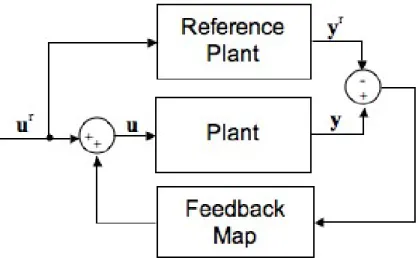
k does not depend on future observations. A special case of the controller in (3) is the fixed linear gain feedbackuk=urk+K(yk−ykr). The feedback structure is illustrated in Figure 1.
In the path planning problem, we plan over a finite horizon of time instances from k= 0 tok=T. For notational convenience we ‘lift’ the variables of interest over the time horizon using the following definitions:
X= x0 x1 .. . xT Xr= xr0 xr 1 .. . xr T Y= y0 y1 .. . yT Yr= y0r yr 1 .. . yr T U= u0 u1 .. . uT Ur= ur0 ur 1 .. . ur T W= w0 w1 .. . wT. (4)
Figure 1. Control structure for robust path planning problem with stochastic plant. The feedforward control is used to set the reference state value, while feedback control is used to drive the system state to the reference value in the presence of noise.
The initial state mean and covariance are denoted ¯x0 andP0respectively. The mean and covariance of the noise sequenceWare denoted ¯WandV respectively. The open-loop lifted system dynamics are given by:
X=Gxxx0+GxuU+GxwW
Y=Gyxx0+GyuU+GywW, (5)
and the open loop lifted reference dynamics are given by:
Xr=Gxx¯x0+GxuUr+GxwW¯
Yr=Gyxx¯0+GyuUr+GywW¯, (6)
where the matrices Gxx,Gxu, Gxw, Gyx, Gyu andGyw are calculated through repeated application of the
system definition (1). Note that, since the dynamics equations (5) are linear, we have E[X] = Xr and
E[Y] =Yr. The control structure can be expressed asU=Ur+K(Y−Yr), where:
K= K00 O · · · O K10 K11 · · · O .. . ... ... KN0 KN1 · · · KN N . (7)
The lower block triangular structure ofK ensures that the controller is non-anticipating. We denote the set of all possible lower block triangular matrices of the form (7) asK.
We define a feasible region Fx ⊂ <nx·(T+1) in the space of the lifted state X, and a feasible region
Fu⊂ <nu·(T+1) in the space of the lifted control inputsU, both of whichmay be nonconvex. We also define
a cost h(Ur,
Xr), and assume thath(·) is a piecewise linear function. The path planning problem may now
be stated as:
Definition 1. Thechance constrained path planning problemconsists of solving the following optimization problem:
Minimize h(Ur,Xr)overUr andK
subject to
Ur∈Fu
P(X∈/Fx)≤δ
III.
Summary of existing work
In Section IV we describe a new algorithm for solving the chance constrained path planning problem (Def. 1). The new algorithm builds from two prior algorithms that solve special cases of the problem in Def. 1. The first uses Mixed Integer Linear Programming (MILP) to perform path planning for deterministic linear systems. While this approach can deal with nonconvex feasible regions, itdoes not take into account uncertainty. The second uses convex optimization to solve chance constrained feedback control problems for stochastic linear systemsin convex regions. In the following sections we describe the key properties of these two approaches as they relate to the new nonconvex robust path planning algorithm.
A. Nonrobust Path Planning using MILP
Definition 2. Thenonrobust path planning problemconsists of solving the following optimization problem:
Minimize h(Ur,Xr)overUr subject to
Ur∈Fu
Xr∈Fx
(6)
Compared with the robust path planning problem (Def. 1), the key difference in Def. 2 is that we are only concerned with the reference state trajectory. The reference state trajectory is deterministic, that is, it does not model any sources of uncertainty. This means that in Def. 2, we constrain the reference system state to remain within the feasible region with certainty. In addition, we no longer design a feedback law, since feedback is only necessary to drive the actual state to the reference state in the presence of uncertainty.
Ref. 6 shows that, in the case of polygonal feasible regions, the nonrobust path planning problem can be posed as a Mixed Integer Linear Program. Efficient commercially-available software17 enables fast solution
of the resulting MILP, and guarantees that the globally optimal solution can be found in bounded time. The key idea behind the approach of Ref. 6 is to encode obstacle avoidance constraints as disjunctions of linear constraints. These disjunctions can be expressed in a MILP formulation using binary variables and ‘Big-M’ techniques as follows.
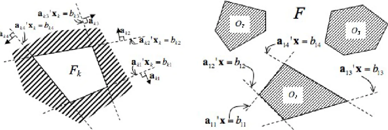
A polygonal convex feasible region can be expressed as a conjunction of linear constraints, as illustrated in Figure 2. The system state at time stepkis in the feasible region if and only if:
^
l
a0klxrk ≤bkl (8)
Using such constraints we can ensure that the system state ends in a defined goal region, and remains in a convex safe region at all time steps. An arbitrary polygonal non-convex feasible region can be described by removing convex infeasible regions, or obstacles, from the safe region, as illustrated in Figure 2. The reference trajectory avoids a given obstacleOj, illustrated in Figure 2, if and only if:
^
k
_
l
a0jlxrk≥bjl (9)
Then the state is in the nonconvex feasible region if and only if: ^ j ^ k _ l a0jlxrk ≥bjl ^^ k ^ l a0klxrk≤bkl (10)
The challenge is to encode the disjunctions in (9). As shown by Ref. 6, in order to encode avoidance of obstacleOj, we introduce binary variablesz(j, k, l)∈ {0,1} that indicate whether a given constraintl for a
given obstacleOj is satisfied at a given time stepk. The constraint:
Figure 2. Left: Polygonal convex feasible regionFk for the state at time stepkencoded using a conjunction of linear constaints. The state is in the feasible region if all of the linear constraints are satisfied. Right: Two-dimensional non-convex polygonal feasible regionF. The feasible region is the complement of several convex obstacles (shaded). Each obstacleOjis defined by theNjvector normalsaj1, . . . ,ajNj.
means thatz(j, k, l) = 0 implies that constraintlin obstacleOj is satisfied at time stepk. HereM is a large
positive constant. We can now encode constraint (9) in terms of the binary variables as follows:
Nj X
l=1
z(j, k, l)≤Nj−1 ∀k. (12)
By imposing the constraint (12) for all obstacles, we ensure that all obstacles are avoided at all time steps. Using further binary variables we can encode nonconvex constraints on the reference control input sequence
Ur. Hence the constraintsUr∈FuandXr∈Fxare encoded as linear constraints involving binary variables.
The dynamics constraints (6) are linear, and the cost functionh(Ur,Xr) is linear. Hence the nonrobust path
planning problem (Def. 2) is a MILP, and can be solved to global optimality.
We denote the set of all binary variables z(·) as ZZ. Note that each full assignment toZZcorresponds to a convex polygonal region that is a subset of the full nonconvex feasible space. The MILP solution of the nonrobust path planning problem therefore returns not only the optimal control sequenceUr, but also the
convex region of Fx in which the optimal reference trajectory Xr was found. We use this property in our
new algorithm for robust path planning, described in Section IV. For notational convenience in this paper, we define the function that solves the nonrobust path planning problem using MILP in Table 1.
FunctionNonRobustPathPlanning(Fx, Fu)returnsh,Uˆr,ZZ
1) Express the polygonal nonconvex regionFx in a Mixed Integer Linear format
using (11) and (12).
2) Solve the optimization problem in Def. 2 for ˆUrandZZusing MILP techniques,
as described by Ref. 6.
Table 1. Nonrobust Path Planning using MILP.
B. Robust Control Design using Convex Optimization
Definition 3. The chance constrained convex planning problemconsists of solving the following optimiza-tion problem:
Minimize h(Ur,Xr)overUr andK
subject to
Ur∈Fu
P(X∈/Fx)≤δ
Fu, Fx convex
This is identical to the chance constrained path planning problem (Def. 1) except that the feasible sets Fu
and Fx are restricted to being convex. This problem was addressed in a series of recent articles11–14 and
expanded upon in Ref. 15. This work determines the distance of the reference stateXrfrom the boundaries
ofFxsufficient to ensure that the chance constraint P(X∈/Fx)≤δis satisfied for anyδ≤0.5. This enables
the chance constraintP(X∈/ Fx)≤δto be approximated as a constraint on theXr, which is not a random
variable. The problem in Def. 3 is then approximated as follows:
Definition 4. The conservative convex planning problem consists of solving the following optimization problem:
Minimize h(Ur,Xr)overUr andK
subject to
Ur∈Fu
Xr+E(K, δ)⊂Fx
Fu, Fx convex
(3),(5),(6),(7), (14)
whereE(r, K, δ)is an ellipsoid defined such that:
P X∈ {/ Xr+E(r, K, δ)}
≤δ. (15)
From (15) and Def. 4 we see that satisfaction of the constraintXr+E(r, K, δ)⊂F
ximplies satisfaction of the
chance constraint P(X∈/ Fx)≤δ. Hence a feasible solution to the conservative chance constrained convex
planning problem (Def. 4) is a feasible solution to the chance constrained convex planning problem (Def. 3). Ref. 15 shows that the optimization in Def. 4 can be posed as a Second-Order Cone Program (SOCP). The details of this are shown in the Appendix. An SOCP is an example of a convex optimization problem, for which fast algorithms exist with guaranteed convergence to global optimality, with known bounds on the convergence rate.16 Hence the approximation of the chance constrained convex planning problem can
be solved efficiently. However the ellipsoidal approximation of the chance constraint in Def. 4 introduces conservatism; this introduces suboptimality in the returned solution. In the general case there exist non-ellipsoidal sets that satisfy (15) but that yield a lower cost solution to the Def. 4; however the ellipsoid constraint is required to pose the problem as an SOCP. For notational simplicity, we define the function that solves the conservative convex planning problem using MILP in Table 2.
FunctionConservativeConvexPlanning(Fx, Fu, δ)returnsh,Ur, K
1) Express the conservative convex planning problem in Def. 4 as a SOCP using the approach in the Appendix.
2) Solve the SOCP using existing techniques16 for the optimal solution{Ur, K}
with costh.
Table 2. Nonrobust Path Planning using MILP.
IV.
A New Algorithm for Robust Path Planning
In this paper we extend the work of Ref. 15 to the case of nonconvex feasible regions, in other words to path planning with obstacles. We use the results of Ref. 15 to approximate the chance constraints in a conservative manner. This results in the following approximation of the chance constrained path planning problem:
Definition 5. Theconservative path planning problemconsists of solving the following optimization prob-lem:
Minimize h(Ur,Xr)overUr andK
subject to
Ur∈Fu
Xr+E(r, K, δ)⊂Fx
From the result of Ref. 15, any feasible solution to the conservative path planning problem (Def. 5) is guaranteed to be a feasible solution to the chance constrained path planning problem (Def. 4). Note that the only difference between Def. 5 and Def. 4 is that the feasible regions are no longer required to be convex. The extension of the algorithm proposed by Ref. 15 to the nonconvex case, however, is far from trivial. The tractability of the conservative convex planning problem (Def. 4) is crucially dependent on the convexity of the sets Fu and Fx. If either of these are nonconvex, the resulting optimization is nonlinear
and nonconvex. Finding the globally optimal solution of such a problem is intractable in the general case; existing algorithms provide, in practice, convergence to local optima and hence require good initial guesses for acceptable performance.
An alternative approach would be to pose the conservative path planning problem as a Mixed Integer Convex Program (MICP). As in Section III-A, nonconvex polygonal constraints can be encoded using binary variables. For a given assignment to the binary variables, the constraints are convex, and we therefore have an MICP. Recent development in solver technology has enabled the solution of such problems, using convex optimizers to solve convex subproblems, and branch-and-bound to search the nonconvex space for the globally optimal solution efficiently. For path planning problems of interest, however, the resulting MICPs are too large to be tractable. We therefore require a new, tractable algorithm for solving the conservative path planning problem. In this section we describe such an algorithm.
A. Algorithm Description
The key idea behind the new algorithm is to use the approaches of Ref. 6 and Ref. 15 to solve subproblems of the chance constrained path planning problem in such a manner that we achieve good average-case performance while guaranteeing convergence to a global optimum in finite time. Since the nonrobust path planning problem (Def. 2) is a MILP, it can be solved extremely quickly. The conservative convex planning problem (Def. 4) is significantly slower to solve. Intuitively, however, the optimal robust solution is close to the optimal nonrobust solution in many cases. In addition, the optimal nonrobust cost is a lower bound on the optimal robust cost, as we prove in Section IV-B. We therefore use the nonrobust solution to guide the search for a robust solution in two ways; first, to identify promising regions in which to search for a robust solution; second, to terminate the search by certifying that the robust solution cannot improve.
The algorithm proceeds as follows. First we solve the nonrobust problem and identify the convex region in which the optimal solution was found. We then look for a robust solution in this convex feasible region using the conservative convex planning approach of Ref. 15, described in Section III-B. Using the results of the robust optimization we remove regions of the nonconvex feasible region in which we know the robust cost cannot improve. The algorithm then starts another iteration by solving the nonrobust problem in the diminished nonconvex feasible space. This proceeds until the optimal nonrobust cost is greater than the best robust cost found so far. Since the optimal nonrobust cost is a lower bound on the robust cost in the remaining feasible space, we are guaranteed at this point to have found the globally optimal robust solution. As we demonstrate empirically in Section V, the algorithm finds the globally optimal solution quickly, and then spends the rest of its running time proving that the solution found is indeed globally optimal. Pseudocode for the algorithm is given in Table 3. In Section B we prove that the algorithm reaches a global optimum in finite time.
B. Algorithm Properties
Lemma 1 (Conservative Cost Greater than Nonrobust Cost). Fix all problem parameters includ-ing the feasible regionsFxand Fu. Denote the cost of the optimal solution to the nonrobust path planning
problem (Def. 2) as ˆh. Denote the cost of the optimal solution to the conservative path planning problem (Def. 5) as h∗. If no feasible solution exists, the optimal cost is defined as infinity. Then, for any δ≤0.5, we havehˆ≤h∗.
Proof: In the nonrobust path planning problem, the state constraints ensure that the reference state is inside the feasible region, i.e. Xr∈F
x. The conservative path planning problem withδ≤0.5 ensures that
the reference state is at least a certain backoff distance r >0 from the boundaries ofFx. Hence the state
constraints are strictly tighter in the conservative path planning problem. Other than this, the two problems are identical. Hence the conservative cost cannot be less than the nonrobust cost; equality occurs when the
Figure 3. Illustration of new approach to chance constrained path planning. a) First, a nonrobust optimal solution is found, which does not take into account uncertainty. The algorithm identifies the convex regionC in which this solution lies. b) The algorithm searches for a chance constrained (robust) solution inC(note that a region convex in the lifted vectorXappears non-convex in the
figure). No robust solution exists in theC. We remove from the search space a region guaranteed not to contain a feasible robust solution. c) We search for a nonrobust optimal solution, which this times avoids the narrow corridor. d) A robust feasible solution does exist in the convex region about the solution in c). This becomes our new incumbent solution. Our next nonrobust solution has cost greater than our incumbent cost. Since this is a lower bound on the robust cost in the remaining search space, we have guaranteed optimality.
Lemma 1 says that the conservative cost is never less than the nonrobust cost for a given set of problem parameters. Following directly from this, we have ˆh= ∞ =⇒ h∗ = ∞ and h∗ <∞ =⇒ ˆh < ∞. In other words, if the nonrobust problem is infeasible, then the conservative problem is infeasible, and if the conservative problem is feasible, then the nonrobust problem is feasible.
Lemma 2 (Pruning). At iteration i, the function PruneSearchSpace does not remove any feasible solution with cost better than˜hi.
Proof: The functionPruneSearchSpaceidentifies which of the obstacle constraints are tight in the opti-mal conservative solution, which has cost ˜hi. We denote this subsettight constraints. PruneSearchSpace
removes the part of the nonconvex search space for whichtight constraintsare imposed. Any conservative path planning problem withtight constraints imposed will have an optimal cost no better than ˜hi. Hence
any feasible solution removed byPruneSearchSpacehas cost no better than ˜hi.
Theorem 1 (Global Optimality). The algorithm described in Table 3 terminates only if the globally optimal feasible solution has been found, or no feasible solution exists.
Proof: The algorithm starts with a nonconvex feasible state region Fx. At each iteration i, in Step 9, a
subsetPi of the feasible region is removed, leaving a regionFx0. From Lemma 2 we know that for eachi, ˜hi
is the minimum cost in Pi. We set h∗ to ˜hi if and only if ˜hi < h∗, so h∗ = mini˜hi. Hence at Step 9, we
know that h∗ is the minimum cost feasible solution in the setR :=Si
j=1Pj. That is, our incumbent cost
is guaranteed to be no worse than any feasible solution in the search space explored so far. The algorithm terminates at iteration j only if ˆhj ≥h∗. The nonrobust cost ˆhj is the optimal nonrobust solution in the
remaining (possibly nonconvex) feasible regionFx0. From Lemma 1 we know that the optimal conservative cost inFx0 is no less than ˆhj. Hence any conservative feasible solution inFx0 has no better cost thanh∗. Since
we knowh∗ is the minimum of all conservative feasible costs in R, and that R∪Fx0 =Fx, at termination
h∗ is the globally optimal cost in Fx. If the globally optimal cost is infinite, then no conservative feasible
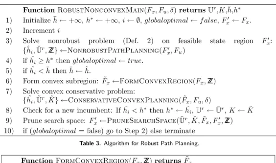
FunctionRobustNonconvexMain(Fx, Fu, δ)returnsUr,K,¯h,h∗
1) Initialize ¯h←+∞,h∗←+∞, i← ∅, globaloptimal←f alse,Fx0 ←Fx.
2) Incrementi
3) Solve nonrobust problem (Def. 2) on feasible state region Fx0:
{ˆhi,Uˆr,ZZ} ←NonrobustPathPlanning(Fx0, Fu) 4) if ˆhi≥h∗thenglobaloptimal←true.
5) if ˆhi<¯hthen ¯h←hˆ.
6) Form convex subregion: ˜Fx←FormConvexRegion(Fx,ZZ)
7) Solve convex conservative problem:
{h˜i,U˜r,K} ←˜ ConservativeConvexPlanning( ˜Fx, Fu, δ)
8) Check for a new incumbent: If ˜hi < h∗ thenh∗←h˜i,Ur←U˜r,K←K˜
9) Prune search space: Fx0 ←PruneSearchSpace(U˜r,K,˜ F˜x, Fx0,ZZ)
10) if (globaloptimal= false) go to Step 2) else terminate Table 3. Algorithm for Robust Path Planning. FunctionFormConvexRegion(Fx,ZZ)returnsF˜x
1) Express nonconvex region Fx in Mixed Integer Linear format as described in
Section A.
2) Assign binary variables in Fx to those in ZZ. Denote the resulting convex
polygonal region ˜Fx.
Table 4. Function to form convex region from MILP solution.
Lemma 3 (Finite Time). The algorithm described in Table 3 is guaranteed to terminate in bounded time.
Proof: The polygonal nonconvex feasible state region Fx is defined by a disjunction of linear constraints.
At each iteration ofRobustNonconvexMain, a region defined by subsets of these linear constraints are removed from the search space. Since there are a countable number of linear constraints, there are a countable number of such subsets. If all constraint subsets are removed, the nonrobust problem becomes infeasible and ˆ
hi=∞, at which point the algorithm terminates. Hence termination is guaranteed in bounded time.
V.
Simulation Results
The algorithmRobustNonconvexMainwas applied to a problem of chance constrained path planning for a UAV in a 2D environment with uncertain localization acting under wind disturbances. Following the approach of Ref. 6 we model the aircraft as a double integrator with velocity limits and turn rate constraints.
FunctionPruneSearchSpace( ˜Ur,K,˜ F˜x, Fx0,ZZ)returnsFx0
1) Determine which constraints defining the convex set ˜Fxare tight in the optimal
solution{U˜r,K}˜ by finding those constraints with nonzero dual values.
2) Determine the subset of the binary variables ZZ corresponding to these con-straints. In other words, determine which variables in ZZ were set to zero to enforce the tight constraints. Denote the vector of these variablesZZsub. 3) Remove fromFx0 the region for which every binary inZZsubis zero. This is
equiv-alent to adding to the MILP formulation ofFx0 the constraintsum(ZZsub)≥1. Table 5. Function to remove region from nonconvex search space.
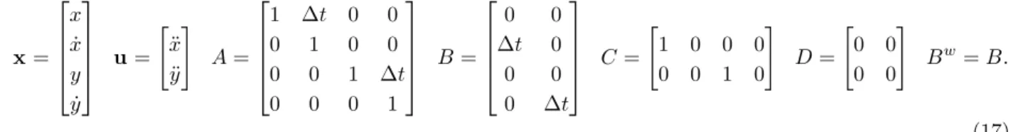
Denoting the position vector of the UAV as [x y]0, the system is defined as: x= x ˙ x y ˙ y u= " ¨ x ¨ y # A= 1 ∆t 0 0 0 1 0 0 0 0 1 ∆t 0 0 0 1 B = 0 0 ∆t 0 0 0 0 ∆t C= " 1 0 0 0 0 0 1 0 # D= " 0 0 0 0 # Bw=B. (17) Initially the UAV is moving North with velocity 0.5m/s. Localization uncertainty is modeled by Gaussian uncertainty in the initial statex0while wind disturbances are modeled as Gaussian white process noise. The statistics of these random variables are given by:
¯ x0= 0 0 0 0.5 P0= 2.5×10⁻³ 0 0 0 0 2.5×10⁻⁷ 0 0 0 0 2.5×10⁻³ 0 0 0 0 2.5×10⁻⁷ ¯ w= " 0 0 # var(w) = " 4 0 0 1 # ×10−5. (18) The maximum velocity of the UAV is 1.0m/sand the maximum acceleration is 0.25m/s2. These magnitude constraints were approximated using an 8-sided inscribing polygon as described by Ref. 7. A time horizon of 10 steps was used, with ∆t= 2s. We constrain the system state to be in the goal region at the final time step, and to avoid all obstacles at all time steps. In the optimizations we minimize fuel use, defined as:
f uel= N X k=0 |x¨k|+|y¨k| . (19)
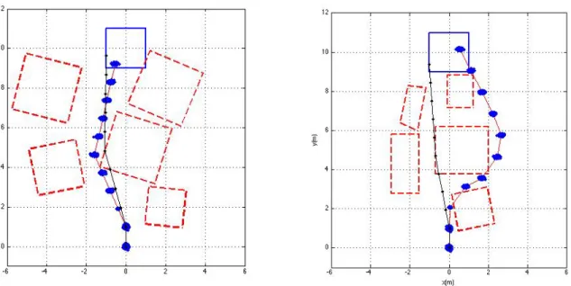
We implemented theRobustNonconvexMainalgorithm in Matlab using the YALMIP interface. The GLPK package was used to solve MILP problems, while SPDT3 was used to solve SOCP problems. The results shown here were generated on a 2.4GHz Macbook Pro with 4GB of RAM. Figure 4 shows the globally optimal robust path found byRobustNonconvexMain for two different obstacle maps with a maximum probability of failure of 0.01. One of these maps is easy for the RobustNonconvexMain algorithm, because the optimal robust solution is close to the optimal nonrobust solution. The other is hard, because the optimal nonrobust solution travels through a narrow corridor too risky for a robust solution. This means that RobustNonconvexMainhas to spend more time searching for the optimal robust solution. We use these examples to illustrate the performance of the algorithm at two extremes.
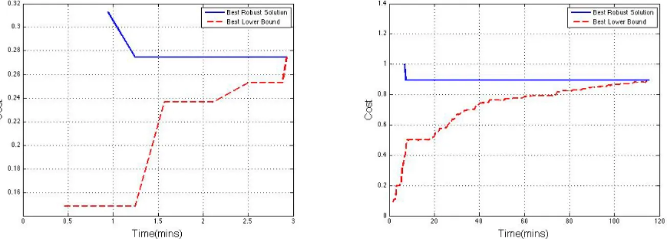
Figure 5 shows the convergence ofRobustNonconvexMainalgorithm to the globally optimal solution. We show the cost of the best robust feasible solution found so far and the best lower bound on the robust feasible cost. The lower bound is provided by the cost of nonrobust feasible solutions. Global optimality is proven when the gap between the two values reaches zero. Figure 5 shows that the easy map yields a provably optimal solution in 2.9minswhereas the hard map requires 118mins. Notice that in both cases the globally optimal solution is found in a small fraction of the total running time; the majority of time is spent
proving global optimality. This suggests that, in practice, the algorithm can be terminated early without a substantial deterioration in the returned solution.
The true probability of failure for the globally optimal solutions in Figure 4 was estimated by performing 108 Monte-Carlo simulations. For both the specified maximum probability of failure was 0.01, however the true value was far below this; the easy map had a probability of failure of 1.0×10⁻⁶ and the hard map had a probability of failure of 5.0×10⁻⁷. This indicates a high level of conservatism, which arises from the bounding approach used in the ConservativeConvexPlanning method of Ref. 15. Reducing this conservatism while guaranteeing chance constrained satisfaction is an open problem.
VI.
Conclusion
In this paper we presented a novel method for optimal chance constrained path planning with feedback design. Unlike previous approaches to chance constrained path planning, the new approach optimizes the feedback gain as well as the reference trajectory. The new approach couples a fast, nonconvex solver that
Figure 4. Globally optimal robust solutions for easy (left) and hard (right) maps. The reference trajectory is shown in red (thin) and the distribution of the position is represented using1000random samples. Also shown in black (thin) is the optimal nonrobust solution. In the easy map the optimal robust solution is close to the optimal nonrobust solution, so the algorithm terminates quickly. in the hard map the narrow corridor at[−1,5]means that the optimal robust solution is far from the optimal nonrobust solution. Nevertheless the algorithm eventually finds the optimal robust solution. In this exampleδ= 0.01. Note that the state constraints are only imposed at the discretization points; obstacle ‘jumpovers’ can be avoided by standard tightening approaches.18
does not take into account uncertainty, with existing robust approaches that apply only to convex feasible regions. By alternating between robust and nonrobust solutions, the new algorithm guarantees convergence to a global optimum. We apply the new method to the problem of robust path planning for a UAV and show that the algorithm finds the globally optimal robust solution early, before performing additional computation to prove global optimality.
Appendix
Here we provide details of the Second Order Cone Program that is equivalent to the conservative convex planning problem (Def. 4). For details of the derivation, refer to Ref. 15. First, define:
Q=K(I−GyuK)−1. (20)
Now define a polygonal feasible region forXas a conjunction of linear constraints:
^
j=1:N
a0jX≥bj. (21)
As shown by Ref. 15, the problem in Def. 4 is equivalent to the Second Order Cone Program given by: Minimizeh(Ur,Xr) overUrandQ
subject to Ur∈Fu Q∈ K νj(Q) +a0jX r ≤bj ∀j νj(Q) =r||a0j[(Gxx+GxuQGyx)FP) (Gxw+GxuQGyw)FW]||2 ∀j Xr=Gxxx0¯ +GxuUr+GxwW¯, (22) whereFP = √ P0and FW = √ V.
Figure 5. Convergence ofRobustNonconvexMainalgorithm to globally optimal solution for easy map (left) and hard map (right). Shown are the cost of the best robust feasible solution found and the best lower bound on the robust feasible solution. In both cases the globally optimal solution is found early in the process, with the majority of time being used to prove global optimality.
Acknowledgement
The research described in this paper was carried out in part at the Jet Propulsion Laboratory, California Institute of Technology, under a contract with the National Aeronautics and Space Administration.
References
1Zhou, K. and Doyle, J. C.,Essentials of Robust Control, Prentice Hall, 1997.
2Bemporad, A. and Morari, M., “Robust Model Predictive Control: A Survey,” In Robustness in Identification and
Control, edited by A. T. A. Garulli and A. Vechino, Springer-Verlag, 1999, pp. 207–226.
3A¸cıkme¸se, B. and Carson, J. M., “A Nonlinear Model Predictive Control Algorithm with Proven Robustness and
Resolv-ability,”Proceedings of the American Control Conference, June 2006, pp. 887–893.
4Carson, J. and A¸cıkme¸se, B., “A model predictive control technique with guaranteed resolvability and required thruster
silent times for small-body proximity operations,”AIAA Guidance, Navigation, and Control Conference and Exhibit, August 2006.
5Barr, N. M., Gangsaas, D., and Schaeffer, D. R., “Wind Models for Flight Simulator Certification of Landing and
Approach Guidance and Control Systems,” Paper FAA-RD-74-206, 1974.
6Schouwenaars, T., Moor, B. D., Feron, E., and How, J., “Mixed Integer Programming for Multi-Vehicle Path Planning,”
Proc. European Control Conference, 2001.
7Richards, A. and How, J., “Aircraft Trajectory Planning with Collision Avoidance Using Mixed Integer Linear
Program-ming,”Proc. American Control Conference, 2002.
8Blackmore, L., Li, H. X., and Williams, B. C., “A Probabilistic Approach to Optimal Robust Path Planning with
Obstacles,”Proceedings of the American Control Conference, 2006.
9Blackmore, L., “A Probabilistic Particle Control Approach to Optimal, Robust Predictive Control,”Proceedings of the
AIAA Guidance, Navigation and Control Conference, 2006.
10Blackmore, L., Bektassov, A., Ono, M., and Williams, B. C., “Robust, Optimal Predictive Control of Jump Markov
Linear Systems using Particles,”Hybrid Systems: Computation and Control, HSCC, edited by A. Bemporad, A. Bicchi, and G. Buttazzo, Vol. 4416 ofLecture Notes in Computer Science, Springer Verlag, 2007, pp. 104–117.
11van Hessem, D., Scherer, C. W., and Bosgra, O. H., “LMI-based closed-loop economic optimization of stochastic process
operation under state and input constraints,”Proceedings of the Control and Decision Conference, 2001.
12van Hessem, D. and Bosgra, O. H., “Closed-loop stochastic dynamics process optimization under state and input
con-straints,”Proceedings of the Control and Decision Conference, 2002.
13van Hessem, D. and Bosgra, O. H., “A full solution to the constrained stochastic closed-loop MPC problem via state and
innovations feedback and its receding horizon implementation,”Proceedings of the Control and Decision Conference, 2003.
14van Hessem, D. and Bosgra, O. H., “Closed-loop stochastic model predictive control in a receding horizon implementation
on a continuous polymerization reactor example,”Proceedings of the Control and Decision Conference, 2004.
15Hessem, D. H. V., Stochastic Inequality Constrained Closed-loop Model Predictive Control, Ph.D. thesis, Technische
Universiteit Delft, Delft, The Netherlands, 2004.
16Boyd, S. and Vandenberghe, L.,Convex Optimization, Cambridge University Press, 2004. 17ILOG, “ILOG CPLEX User’s guide,” 1999.
18Kuwata, Y., Trajectory Planning for Unmanned Vehicles using Robust Receding Horizon Control, Ph.D. thesis,