Unbiased Estimation
14.1 Introduction
In creating a parameter estimator, a fundamental question is whether or not the estimator differs from the parameter in a systematic manner. Let’s examine this by looking a the computation of the mean and the variance of 16 flips of a fair coin.
Give this task to 10 individuals and ask them report the number of heads. We can simulate this inRas follows > (x<-rbinom(10,16,0.5))
[1] 8 5 9 7 7 9 7 8 8 10
Our estimate is obtained by taking these 10 answers and averaging them. Intuitively we anticipate an answer around 8. For these 10 observations, we find, in this case, that
> sum(x)/10 [1] 7.8
The result is a bit below 8. Is this systematic? To assess this, we appeal to the ideas behind Monte Carlo to perform a 1000 simulations of the example above.
> meanx<-rep(0,1000)
> for (i in 1:1000){meanx[i]<-mean(rbinom(10,16,0.5))} > mean(meanx)
[1] 8.0049
From this, we surmise that we the estimate of the sample mean x¯ neither systematically overestimates or un-derestimates the distributional mean. From our knowledge of the binomial distribution, we know that the mean
µ=np= 16·0.5 = 8. In addition, the sample meanX¯ also has mean EX¯ = 1
10(8 + 8 + 8 + 8 + 8 + 8 + 8 + 8 + 8 + 8) = 80 10 = 8 verifying that we have no systematic error.
The phrase that we use is that the sample meanX¯ is anunbiasedestimator of the distributional meanµ. Here is the precise definition.
Definition 14.1. For observationsX= (X1, X2, . . . , Xn)based on a distribution having parameter value✓, and for
d(X)an estimator forh(✓), thebiasis the mean of the differenced(X) h(✓), i.e.,
bd(✓) =E✓d(X) h(✓). (14.1) Ifbd(✓) = 0for all values of the parameter, thend(X)is called anunbiased estimator. Any estimator that is not
Example 14.2. LetX1, X2, . . . , Xn be Bernoulli trials with success parameterpand set the estimator forpto be
d(X) = ¯X, the sample mean. Then,
EpX¯ = 1
n(EX1+EX2+· · ·+EXn) =
1
n(p+p+· · ·+p) =p
Thus,X¯ is an unbiased estimator forp. In this circumstance, we generally writepˆinstead ofX. In addition, we can¯
use the fact that for independent random variables, the variance of the sum is the sum of the variances to see that
Var(ˆp) = 1
n2(Var(X1) +Var(X2) +· · ·+Var(Xn)) = 1
n2(p(1 p) +p(1 p) +· · ·+p(1 p)) = 1
np(1 p).
Example 14.3. IfX1, . . . , Xn form a simple random sample with unknown finite mean µ, thenX¯ is an unbiased
estimator ofµ. If theXihave variance 2, then
Var( ¯X) = 2
n . (14.2)
We can assess the quality of an estimator by computing itsmean square error, defined by
E✓[(d(X) h(✓))2]. (14.3)
Estimators with smaller mean square error are generally preferred to those with larger. Next we derive a simple relationship between mean square error and variance. We begin by substituting (14.1) into (14.3), rearranging terms, and expanding the square.
E✓[(d(X) h(✓))2] =E✓[(d(X) (E✓d(X) bd(✓)))2] =E✓[((d(X) E✓d(X)) +bd(✓))2] =E✓[(d(X) E✓d(X))2] + 2bd(✓)E✓[d(X) E✓d(X)] +bd(✓)2 =Var✓(d(X)) +bd(✓)2
Thus, the representation of the mean square error as equal to the variance of the estimator plus the square of the bias is called thebias-variance decomposition. In particular:
• The mean square error for an unbiased estimator is its variance.
• Bias always increases the mean square error.
14.2 Computing Bias
For the variance 2, we have been presented with two choices: 1 n n X i=1 (xi x¯)2 and 1 n 1 n X i=1 (xi x¯)2. (14.4)
Using bias as our criterion, we can now resolve between the two choices for the estimators for the variance 2. Again, we use simulations to make a conjecture, we then follow up with a computation to verify our guess. For 16 tosses of a fair coin, we know that the variance isnp(1 p) = 16·1/2·1/2 = 4
For the example above, we begin by simulating the coin tosses and compute the sum of squaresP10
i=1(xi x¯)2, > ssx<-rep(0,1000)
> for (i in 1:1000){x<-rbinom(10,16,0.5);ssx[i]<-sum((x-mean(x))ˆ2)} > mean(ssx)
Histogram of ssx ssx F re qu en cy 0 20 40 60 80 100 120 0 50 100 150 200 250
Figure 14.1: Sum of squares aboutx¯for 1000 simulations.
The choice is to divide either by 10, for the first choice, or 9, for the second.
> mean(ssx)/10;mean(ssx)/9 [1] 3.58511
[1] 3.983456
Exercise 14.4. Repeat the simulation above, compute the sum of squaresP10
i=1(xi 8)2. Show that these
sim-ulations support dividing by 10 rather than 9. verify that Pn
i=1(Xi µ)2/nis an unbiased estimator for 2for
in-dependent random variableX1, . . . , Xnwhose common
distribution has meanµand variance 2.
In this case, because we know all the aspects of the simulation, and thus we know that the answer ought to be near 4. Consequently, division by 9 appears to be the appropriate choice. Let’s check this out, beginning with what seems to be theinappropriate choiceto see what goes wrong..
Example 14.5. If a simple random sampleX1, X2, . . . ,
has unknown finite variance 2, then, we can consider the sample variance
S2= 1 n n X i=1 (Xi X¯)2.
To find the mean ofS2, we divide the difference between an observationX
iand the distributional mean into two steps
- the first fromXito the sample meanx¯and and then from the sample mean to the distributional mean, i.e.,
Xi µ= (Xi X¯) + ( ¯X µ).
We shall soon see that the lack of knowledge ofµis the source of the bias. Make this substitution and expand the square to obtain n X i=1 (Xi µ)2= n X i=1 ((Xi X¯) + ( ¯X µ))2 = n X i=1 (Xi X¯)2+ 2 n X i=1 (Xi X¯)( ¯X µ) + n X i=1 ( ¯X µ)2 = n X i=1 (Xi X¯)2+ 2( ¯X µ) n X i=1 (Xi X¯) +n( ¯X µ)2 = n X i=1 (Xi X¯)2+n( ¯X µ)2
(Check for yourself that the middle term in the third line equals 0.) Subtract the termn( ¯X µ)2from both sides and
divide bynto obtain the identity
1 n n X i=1 (Xi X¯)2= 1 n n X i=1 (Xi µ)2 ( ¯X µ)2.
Using the identity above and the linearity property of expectation we find that ES2=E " 1 n n X i=1 (Xi X¯)2 # =E " 1 n n X i=1 (Xi µ)2 ( ¯X µ)2 # = 1 n n X i=1 E[(Xi µ)2] E[( ¯X µ)2] = 1 n n X i=1 Var(Xi) Var( ¯X) = 1 nn 2 1 n 2= n 1 n 2 6 = 2.
The last line uses (14.2). This shows thatS2is a biased estimator for 2. Using the definition in (14.1), we can
see that it is biased downwards.
b( 2) = n 1
n
2 2= 1
n
2.
Note that the bias is equal to Var( ¯X). In addition, because E n n 1S 2 = n n 1E ⇥ S2⇤= n n 1 ✓n 1 n 2◆= 2 and Su2= n n 1S 2= 1 n 1 n X i=1 (Xi X¯)2
is an unbiased estimator for 2. As we shall learn in the next section, because the square root is concave downward,
Su=
p S2
uas an estimator for isdownwardly biased.
Example 14.6. We have seen, in the case of nBernoulli trials havingxsuccesses, thatpˆ = x/n is an unbiased estimator for the parameterp. This is the case, for example, in taking a simple random sample of genetic markers at a particular biallelic locus. Let one allele denote the wildtype and the second a variant. If the circumstances in which variant is recessive, then an individual expresses the variant phenotype only in the case that both chromosomes contain this marker. In the case of independent alleles from each parent, the probability of the variant phenotype is p2. Na¨ıvely, we could use the estimatorpˆ2. (Later, we will see that this is the maximum likelihood estimator.) To
determine the bias of this estimator, note that
Epˆ2= (Epˆ)2+Var(ˆp) =p2+1
np(1 p). (14.5)
Thus, the biasb(p) =p(1 p)/nand the estimatorpˆ2is biased upward. Exercise 14.7. For Bernoulli trialsX1, . . . , Xn,
1 n n X i=1 (Xi pˆ)2= ˆp(1 pˆ).
Based on this exercise, and the computation above yielding an unbiased estimator,S2
u, for the variance,
E 1 n 1pˆ(1 pˆ) = 1 nE " 1 n 1 n X i=1 (Xi pˆ)2 # = 1 nE[S 2 u] = 1 nVar(X1) = 1 np(1 p).
In other words,
1
n 1pˆ(1 pˆ)
is an unbiased estimator ofp(1 p)/n. Returning to (14.5),
E ˆ p2 1 n 1pˆ(1 pˆ) = ✓ p2+1 np(1 p) ◆ 1 np(1 p) =p 2. Thus, b p2 u= ˆp2 1 n 1pˆ(1 pˆ) is an unbiased estimator ofp2.
To compare the two estimators forp2, assume that we find 13 variant alleles in a sample of 30, thenpˆ= 13/30 = 0.4333, ˆ p2= ✓13 30 ◆2 = 0.1878, and pb2 u= ✓13 30 ◆2 1 29 ✓13 30 ◆ ✓17 30 ◆ = 0.1878 0.0085 = 0.1793. The bias for the estimatepˆ2, in this case 0.0085, is subtracted to give the unbiased estimatepb2
u.
Theheterozygosityof a biallelic locus ish= 2p(1 p). From the discussion above, we see thathhas the unbiased estimator ˆ h= 2n n 1pˆ(1 pˆ) = 2n n 1 ⇣x n ⌘ ✓n x n ◆ =2x(n x) n(n 1) .
14.3 Compensating for Bias
In the methods of moments estimation, we have usedg( ¯X)as an estimator forg(µ). Ifgis aconvex function, we
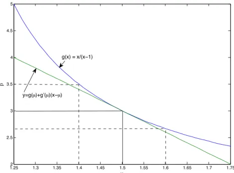
can say something about the bias of this estimator. In Figure 14.2, we see the method of moments estimator for the estimatorg( ¯X)for a parameter in the Pareto distribution. The choice of = 3corresponds to a mean ofµ= 3/2for the Pareto random variables. The central limit theorem states that the sample meanX¯ is nearly normally distributed with mean 3/2. Thus, the distribution ofX¯ is nearly symmetric around 3/2. From the figure, we can see that the interval from 1.4 to 1.5 under the functiongmaps into a longer interval above = 3than the interval from 1.5 to 1.6 maps below = 3. Thus, the functiongspreads the values ofX¯ above = 3more than below. Consequently, we anticipate that the estimatorˆwill beupwardly biased.
To address this phenomena in more general terms, we use the characterization of a convex function as a differen-tiable function whose graph lies above any tangent line. If we look at the valueµfor the convex functiong, then this statement becomes
g(x) g(µ) g0(µ)(x µ).
Now replacexwith the random variableX¯ and take expectations.
Eµ[g( ¯X) g(µ)] Eµ[g0(µ)( ¯X µ)] =g0(µ)Eµ[ ¯X µ] = 0. Consequently,
Eµg( ¯X) g(µ) (14.6)
andg( ¯X)isbiased upwards. The expression in (14.6) is known asJensen’s inequality. Exercise 14.8. Show that the estimatorSuis a downwardly biased estimator for .
To estimate the size of the bias, we look at a quadratic approximation forgcentered at the valueµ g(x) g(µ)⇡g0(µ)(x µ) +1
2g
1.252 1.3 1.35 1.4 1.45 1.5 1.55 1.6 1.65 1.7 1.75 2.5 3 3.5 4 4.5 5 x ! g(x) = x/(x!1) y=g(µ)+g’(µ)(x!µ)
Figure 14.2: Graph of a convex function. Note that the tangent line is below the graph ofg. Here we show the case in whichµ = 1.5and
=g(µ) = 3. Notice that the interval fromx= 1.4tox= 1.5has a longer range than the interval fromx= 1.5tox= 1.6Becausegspreads the values ofX¯above = 3more than below, the estimatorˆfor is biased upward. We can use a second order Taylor series expansion to correct most of this bias.
Again, replacexin this expression with the random variableX¯ and then take expectations. Then, the bias
bg(µ) =Eµ[g( ¯X)] g(µ)⇡Eµ[g0(µ)( ¯X µ)] + 1 2E[g 00(µ)( ¯X µ)2] = 1 2g 00(µ)Var( ¯X) = 1 2g 00(µ) 2 n. (14.7)
(Remember thatEµ[g0(µ)( ¯X µ)] = 0.) Thus, the bias has the intuitive properties of being
• large for strongly convex functions, i.e., ones with a large value for the second derivative evaluated at the mean
µ,
• large for observations having high variance 2, and
• small when the number of observationsnis large.
Exercise 14.9. Use (14.7) to estimate the bias in usingpˆ2as an estimate ofp2is a sequence ofnBernoulli trials and
note that it matches the value (14.5).
Example 14.10. For the method of moments estimator for the Pareto random variable, we determined that g(µ) = µ
µ 1.
and thatX¯ has
mean µ= 1 and variance n2 =n( 1)2( 2)
By taking the second derivative, we see thatg00(µ) = 2(µ 1) 3>0and, becauseµ >1,gis a convex function.
Next, we have g00 ✓ 1 ◆ =⇣ 2 1 1 ⌘3 = 2( 1) 3.
Thus, the bias bg( )⇡ 1 2g 00(µ) 2 n = 1 22( 1) 3 n( 1)2( 2) = ( 1) n( 2).
So, for = 3andn= 100, the bias is approximately 0.06. Compare this to the estimated value of 0.053 from the
simulation in the previous section.
Example 14.11. For estimating the population in mark and recapture, we used the estimate N =g(µ) =kt
µ
for the total population. Hereµis the mean number recaptured,kis the number captured in the second capture event andtis the number tagged. The second derivative
g00(µ) = 2kt
µ3 >0
and hence the method of moments estimate is biased upwards. In this siutation,n= 1and the number recaptured is a
hypergeometric random variable. Hence its variance
2= kt
N
(N t)(N k)
N(N 1) .
Thus, the bias bg(N) =1 2 2kt µ3 kt N (N t)(N k) N(N 1) = (N t)(N k) µ(N 1) = (kt/µ t)(kt/µ k) µ(kt/µ 1) = kt(k µ)(t µ) µ2(kt µ) .
In the simulation example,N = 2000, t= 200, k= 400andµ= 40. This gives an estimate for the bias of 36.02. We
can compare this to the bias of 2031.03-2000 = 31.03 based on the simulation in Example 13.2.
This suggests a new estimator by taking the method of moments estimator and subtracting the approximation of the bias. ˆ N = kt r kt(k r)(t r) r2(kt r) = kt r ✓ 1 (k r)(t r) r(kt r) ◆ .
The delta method gives us that the standard deviation of the estimator is|g0(µ)| /pn. Thus the ratio of the bias
of an estimator to its standard deviation as determined by the delta method is approximately
g00(µ) 2/(2n) |g0(µ)| /pn = 1 2 g00(µ) |g0(µ)|pn.
If this ratio is⌧1, then the bias correction is not very important. In the case of the example above, this ratio is 36.02
268.40 = 0.134 and its usefulness in correcting bias is small.
14.4 Consistency
Despite the desirability of using an unbiased estimator, sometimes such an estimator is hard to find and at other times impossible. However, note that in the examples above both the size of the bias and the variance in the estimator decrease inversely proportional ton, the number of observations. Thus, these estimators improve, under both of these
Definition 14.12. Given dataX1, X2, . . .and a real valued functionhof the parameter space, a sequence of
estima-torsdn, based on the firstnobservations, is calledconsistentif for every choice of✓ lim
n!1dn(X1, X2, . . . , Xn) =h(✓) whenever✓is the true state of nature.
Thus, the bias of the estimator disappears in the limit of a large number of observations. In addition, the distribution of the estimatorsdn(X1, X2, . . . , Xn)become more and more concentrated nearh(✓).
For the next example, we need to recall the sequence definition of continuity: A functiongis continuous at a real
numberxprovided that for every sequence{xn;n 1}with
xn!x, then, we have thatg(xn)!g(x).
A function is called continuous if it is continuous at every value ofxin the domain ofg. Thus, we can write the expression above more succinctly by saying that for every convergent sequence{xn;n 1},
lim
n!1g(xn) =g( limn!1xn).
Example 14.13. For a method of moment estimator, let’s focus on the case of a single parameter (d = 1). For
independent observations,X1, X2, . . . ,having meanµ=k(✓), we have that
EX¯n=µ,
i. e.X¯n, the sample mean for the firstnobservations, is an unbiased estimator forµ=k(✓). Also, by the law of large
numbers, we have that
lim n!1
¯
Xn =µ.
Assume thatkhas a continuous inverseg=k 1. In particular, becauseµ=k(✓), we have thatg(µ) =✓. Next,
using the methods of moments procedure, define, fornobservations, the estimators
ˆ ✓n(X1, X2, . . . , Xn) =g ✓ 1 n(X1+· · ·+Xn) ◆ =g( ¯Xn).
for the parameter✓. Using the continuity ofg, we find that
lim n!1
ˆ
✓n(X1, X2, . . . , Xn) = lim
n!1g( ¯Xn) =g( limn!1X¯n) =g(µ) =✓ and so we have thatg( ¯Xn)is a consistent sequence of estimators for✓.
14.5 Cram´er-Rao Bound
This topic is somewhat more advanced and can be skipped for the first reading. This section gives us an introduction to the log-likelihood and its derivative, thescorefunctions. We shall encounter these functions again when we introduce maximum likelihood estimation. In addition, the Cram´er Rao bound, which is based on the variance of the score function, known as the Fisher information, gives a lower bound for the variance of an unbiased estimator. These concepts will be necessary to describe the variance for maximum likelihood estimators.
Among unbiased estimators, one important goal is to find an estimator that has as small a variance as possible, A more precise goal would be to find an unbiased estimatordthat hasuniform minimum variance. In other words, d(X)has has a smaller variance than for any other unbiased estimatord˜for every value✓of the parameter.
Var✓d(X)Var✓d˜(X) for all✓2⇥.
Theefficiencye( ˜d)of unbiased estimatord˜is the minimum value of the ratio
Var✓d(X) Var✓d˜(X)
over all values of✓. Thus, the efficiency is between 0 and 1 with a goal of finding estimators with efficiency as near to
one as possible.
For unbiased estimators, the Cram´er-Rao bound tells us how small a variance is ever possible. The formula is a bit mysterious at first. However, we shall soon learn that this bound is a consequence of the bound on correlation that we have previously learned
Recall that for two random variablesY andZ, the correlation
⇢(Y, Z) = pCov(Y, Z)
Var(Y)Var(Z). (14.8)
takes values between -1 and 1. Thus,⇢(Y, Z)2
1and so
Cov(Y, Z)2Var(Y)Var(Z). (14.9)
Exercise 14.14. IfEZ= 0, theCov(Y, Z) =EY Z
We begin with dataX = (X1, . . . , Xn)drawn from an unknown probabilityP✓. The parameter space ⇥⇢R. Denote the joint density of these random variables
f(x|✓), wherex= (x1. . . , xn).
In the case that the data comes from a simple random sample then the joint density is the product of the marginal densities.
f(x|✓) =f(x1|✓)· · ·f(xn|✓) (14.10)
For continuous random variables, the two basic properties of the density are thatf(x|✓) 0for allxand that 1 =
Z Rn
f(x|✓)dx. (14.11)
Now, letdbe the unbiased estimator ofh(✓), then by the basic formula for computing expectation, we have for
continuous random variables
h(✓) =E✓d(X) =
Z Rn
d(x)f(x|✓)dx. (14.12)
If the functions in (14.11) and (14.12) are differentiable with respect to the parameter ✓ and we can pass the
derivative through the integral, then we first differentiate both sides of equation (14.11), and then use the logarithm function to write this derivate as the expectation of a random variable,
0 = Z Rn @f(x|✓) @✓ dx= Z Rn @f(x|✓)/@✓ f(x|✓) f(x|✓)dx= Z Rn @lnf(x|✓) @✓ f(x|✓)dx=E✓ @lnf(X |✓) @✓ . (14.13)
From a similar calculation using (14.12),
h0(✓) =E✓
d(X)@lnf(X|✓)
Now, return to the review on correlation withY =d(X), the unbiased estimator forh(✓)and thescore function
Z=@lnf(X|✓)/@✓. From equations (14.14) and then (14.9), we find that
h0(✓)2=E✓ d(X)@lnf(X|✓) @✓ 2 =Cov✓ ✓ d(X),@lnf(X|✓) @✓ ◆ Var✓(d(X))Var✓ ✓@lnf(X |✓) @✓ ◆ , or, Var✓(d(X)) h 0(✓)2 I(✓) . (14.15) where I(✓) =Var✓ ✓@lnf(X |✓) @✓ ◆ =E✓ "✓ @lnf(X|✓) @✓ ◆2#
is called theFisher information. For the equality, recall that the variance Var(Z) =EZ2 (EZ)2and recall from equation (14.13) that the random variableZ=@lnf(X|✓)/@✓has meanEZ= 0.
Equation (14.15), called theCram´er-Rao lower boundor theinformation inequality, states that the lower bound for the variance of an unbiased estimator is the reciprocal of the Fisher information. In other words, thehigherthe information, theloweris the possible value of the variance of an unbiased estimator.
If we return to the case of a simple random sample, then take the logarithm of both sides of equation (14.10) lnf(x|✓) = lnf(x1|✓) +· · ·+ lnf(xn|✓)
and then differentiate with respect to the parameter✓,
@lnf(x|✓) @✓ = @lnf(x1|✓) @✓ +· · ·+ @lnf(xn|✓) @✓ .
The random variables{@lnf(Xk|✓)/@✓; 1kn}are independent and have the same distribution. Using the fact that the variance of the sum is the sum of the variances for independent random variables, we see thatIn, the Fisher information fornobservations isntimes the Fisher information of a single observation.
In(✓) =Var ✓ @lnf(X1|✓) @✓ +· · ·+ @lnf(Xn|✓) @✓ ◆ =nVar(@lnf(X1|✓) @✓ ) =nE[( @lnf(X1|✓) @✓ ) 2].
Notice the correspondence. Informationislinearlyproportional to the number of observations. If our estimator is a sample mean or a function of the sample mean, then the variance isinversely proportional to the number of observations.
Example 14.15. For independent Bernoulli random variables with unknown success probability✓, the density is
f(x|✓) =✓x(1 ✓)(1 x). The mean is✓and the variance is✓(1 ✓). Taking logarithms, we find that
lnf(x|✓) =xln✓+ (1 x) ln(1 ✓), @ @✓lnf(x|✓) = x ✓ 1 x 1 ✓ = x ✓ ✓(1 ✓).
The Fisher information associated to a single observation I(✓) =E "✓ @ @✓lnf(X|✓) ◆2# = 1 ✓2(1 ✓)2E[(X ✓) 2] = 1 ✓2(1 ✓)2Var(X) = 1 ✓2(1 ✓)2✓(1 ✓) = 1 ✓(1 ✓).
Thus, the information fornobservationsIn(✓) =n/(✓(1 ✓)). Thus, by the Cram´er-Rao lower bound, any unbiased
estimator of✓based onnobservations must have variance al least✓(1 ✓)/n. Now, notice that if we taked(x) = ¯x,
then
E✓X¯ =✓, and Var✓d(X) =Var( ¯X) = ✓(1 ✓)
n .
These two equations show thatX¯ is a unbiased estimator having uniformly minimum variance. Exercise 14.16. For independent normal random variables with known variance 2
0 and unknown meanµ,X¯ is a
uniformly minimum variance unbiased estimator.
Exercise 14.17. Take two derivatives oflnf(x|✓)to show that
I(✓) =E✓ "✓ @lnf(X|✓) @✓ ◆2# = E✓ @2lnf(X |✓) @✓2 . (14.16)
This identity is often a useful alternative to compute the Fisher Information. Example 14.18. For an exponential random variable,
lnf(x| ) = ln x, @ 2f(x | ) @ 2 = 1 2. Thus, by (14.16), I( ) = 12. Now,X¯ is an unbiased estimator forh( ) = 1/ with variance
1
n 2.
By the Cram´er-Rao lower bound, we have that g0( )2 nI( ) = 1/ 4 n 2 = 1 n 2.
BecauseX¯ has this variance, it is a uniformly minimum variance unbiased estimator.
Example 14.19. To give an estimator that does not achieve the Cram´er-Rao bound, letX1, X2, . . . , Xnbe a simple
random sample of Pareto random variables with density fX(x| ) =
x +1, x >1.
The mean and the variance
µ= 1,
2=
( 1)2( 2).
Thus,X¯ is an unbiased estimator ofµ= /( 1) Var( ¯X) =
n( 1)2( 2).
To compute the Fisher information, note that
lnf(x| ) = ln ( + 1) lnx and thus @ 2lnf(x | ) @ 2 = 1 2.
Using (14.16), we have that I( ) = 12. Next, for µ=g( ) = 1, g 0( ) = 1 ( 1)2, and g 0( )2= 1 ( 1)4.
Thus, the Cram´er-Rao bound for the estimator is g0( )2
In( ) = 2
n( 1)4.
and the efficiency compared to the Cram´er-Rao bound is g0( )2/In( ) Var( ¯X) = 2 n( 1)4 · n( 1)2( 2) = ( 2) ( 1)2 = 1 1 ( 1)2.
The Pareto distribution does not have a variance unless >2. For just above 2, the efficiency compared to its
Cram´er-Rao bound is low but improves with larger .
14.6 A Note on Efficient Estimators
For an efficient estimator, we need find the cases that lead to equality in the correlation inequality (14.8). Recall that equality occurs precisely when the correlation is±1. This occurs when the estimatord(X)and the score function
@lnfX(X|✓)/@✓are linearly related with probability 1. @
@✓lnfX(X|✓) =a(✓)d(X) +b(✓).
After integrating, we obtain, lnfX(X|✓) =
Z
a(✓)d✓d(X) +
Z
b(✓)d✓+j(X) =⇡(✓)d(X) +B(✓) +j(X)
Note that the constant of integration of integration is a function ofX. Now exponentiate both sides of this equation fX(X|✓) =c(✓)h(X) exp(⇡(✓)d(X)). (14.17)
Herec(✓) = expB(✓)andh(X) = expj(X).
We shall call density functions satisfying equation (14.17) anexponential familywithnatural parameter⇡(✓). Thus, if we have independent random variablesX1, X2, . . . Xn, then the joint density is the product of the densities, namely,
f(X|✓) =c(✓)nh(X1)· · ·h(Xn) exp(⇡(✓)(d(X1) +· · ·+d(Xn)). (14.18)
In addition, as a consequence of this linear relation in (14.18),
d(X) = 1
n(d(X1) +· · ·+d(Xn))
is an efficient estimator forh(✓).
Example 14.20(Poisson random variables).
f(x| ) = x
x!e =e 1
Thus, Poisson random variables are an exponential family withc( ) = exp( ),h(x) = 1/x!, and natural parameter
⇡( ) = ln . Because
=E X,¯
¯
Xis an unbiased estimator of the parameter . The score function
@ @ lnf(x| ) = @ @ (xln lnx! ) = x 1. The Fisher information for one observation is
I( ) =E "✓ X 1 ◆2# = 12E [(X )2] = 1. Thus,In( ) =n/ is the Fisher information fornobservations. In addition,
Var ( ¯X) =
n andd(x) = ¯xhas efficiency
Var( ¯X) 1/In( ) = 1.
This could have been predicted. The density ofnindependent observations is
f(x| ) = e x1! x1· · ·e xn! xn= e n x1···+xn x1!· · ·xn! = e n n¯x x1!· · ·xn!
and so the score function
@
@ lnf(x| ) = @
@ ( n +nx¯ln ) = n+
nx¯
showing that the estimatex¯and the score function are linearly related.
Exercise 14.21. Show that a Bernoulli random variable with parameterpis an exponential family.
Exercise 14.22. Show that a normal random variable with known variance 2
0and unknown meanµis an exponential
family.
14.7 Answers to Selected Exercises
14.4. Repeat the simulation, replacingmean(x)by 8. > ssx<-rep(0,1000)> for (i in 1:1000){x<-rbinom(10,16,0.5);ssx[i]<-sum((x-8)ˆ2)} > mean(ssx)/10;mean(ssx)/9
[1] 3.9918 [1] 4.435333
Note that division by 10 gives an answer very close to the correct value of 4. To verify that the estimator is unbiased, we write E " 1 n n X i=1 (Xi µ)2 # = 1 n n X i=1 E[(Xi µ)2] = 1 n n X i=1 Var(Xi) = 1 n n X i=1 2= 2.
14.7. For a Bernoulli trial note thatX2
i =Xi. Expand the square to obtain n X i=1 (Xi pˆ)2= n X i=1 Xi2 pˆ n X i=1 Xi+npˆ2=npˆ 2npˆ2+npˆ2=n(ˆp pˆ2) =npˆ(1 pˆ). Divide bynto obtain the result.
14.8. Recall thatES2
u= 2. Check the second derivative to see thatg(t) = p
tis concave down for allt. For concave down functions, the direction of the inequality in Jensen’s inequality is reversed. Settingt=Su, we have that2
ESu=Eg(Su2)g(ESu2) =g( 2) = andSuis a downwardly biased estimator of .
14.9. Setg(p) =p2. Then,g00(p) = 2. Recall that the variance of a Bernoulli random variable 2=p(1 p)and the bias bg(p)⇡1 2g 00(p) 2 n = 1 22 p(1 p) n = p(1 p) n . 14.14. Cov(Y, Z) =EY Z EY ·EZ=EY ZwheneverEZ= 0. 14.16. For independent normal random variables with known variance 2
0and unknown meanµ, the density
f(x|µ) = 1 0 p 2⇡exp (x µ)2 2 2 0 , lnf(x|µ) = ln( 0 p 2⇡) (x µ) 2 2 2 0 .
Thus, the score function
@ @µlnf(x|µ) = 1 2 0 (x µ).
and the Fisher information associated to a single observation
I(µ) =E "✓ @ @µlnf(X|µ) ◆2# = 14 0 E[(X µ)2] = 14 0 Var(X) = 12 0 .
Again, the information is the reciprocal of the variance. Thus, by the Cram´er-Rao lower bound, any unbiased estimator based onnobservations must have variance al least 2
0/n. However, if we taked(x) = ¯x, then Varµd(X) =
2 0
n.
andx¯is a uniformly minimum variance unbiased estimator. 14.17. First, we take two derivatives oflnf(x|✓).
@lnf(x|✓) @✓ = @f(x|✓)/@✓ f(x|✓) (14.19) and @2lnf(x |✓) @✓2 = @2f(x |✓)/@✓2 f(x|✓) (@f(x|✓)/@✓)2 f(x|✓)2 = @2f(x |✓)/@✓2 f(x|✓) ✓@f(x |✓)/@✓) f(x|✓) ◆2 = @ 2f(x |✓)/@✓2 f(x|✓) ✓@lnf(x |✓) @✓ ◆2
upon substitution from identity (14.19). Thus, the expected values satisfy E✓ @2lnf(X |✓) @✓2 =E✓ @2f(X |✓)/@✓2 f(X|✓) E✓ "✓@lnf(X |✓) @✓ ◆2# .
Consquently, the exercise is complete if we show thatE✓h@2f(Xf(X|✓|✓)/)@✓2i = 0. However, for a continuous random
variable, E✓ @2f(X |✓)/@✓2 f(X|✓) = Z @2f(x |✓)/@✓2 f(x|✓) f(x|✓)dx= Z @2f(x |✓) @✓2 dx= @2 @✓2 Z f(x|✓)dx= @ 2 @✓21 = 0. Note that the computation require that we be able to pass two derivatives with respect to✓through the integral sign.
14.21. The Bernoulli density
f(x|p) =px(1 p)1 x= (1 p) ✓ p 1 p ◆x = (1 p) exp ✓ xln ✓ p 1 p ◆◆ .
Thus,c(p) = 1 p, h(x) = 1and the natural parameter⇡(p) = ln⇣1pp⌘, thelog-odds. 14.22. The normal density
f(x|µ) = 1 0 p 2⇡exp (x µ)2 2 2 0 = 1 0 p 2⇡e µ2/2 0e x2/2 0expxµ 2 0 Thus,c(µ) = 1 0 p 2⇡e
µ2/2 0, h(x) =e x2/2 0and the natural parameter⇡(µ) =µ/ 2