Louisiana State University
LSU Digital Commons
LSU Master's Theses Graduate School
January 2019
Downscaling SMAP Soil Moisture Data Using
MODIS Data
Le Tu [email protected]
Follow this and additional works at:https://digitalcommons.lsu.edu/gradschool_theses Part of theRemote Sensing Commons, and theSpatial Science Commons
This Thesis is brought to you for free and open access by the Graduate School at LSU Digital Commons. It has been accepted for inclusion in LSU Master's Theses by an authorized graduate school editor of LSU Digital Commons. For more information, please [email protected].
Recommended Citation
Tu, Le, "Downscaling SMAP Soil Moisture Data Using MODIS Data" (2019).LSU Master's Theses. 4847.
i
Downscaling SMAP Soil Moisture Data Using MODIS Data
A Thesis
Submitted to the Graduate Faculty of the Louisiana State University and Agricultural and Mechanical College
in partial fulfillment of the requirements for the degree of
Master of Science in
The Department of Geography and Anthropology
Le Tu
B.A., Anhui University of Architecture, 2016 May 2019
ii
DEDICATION
I dedicate this research first and foremost to my family. They are the biggest inspiration in my life. My parents raise me with love and support, providing me with all they can. My grandparents and great grandparents are my role models of all time. I will always work hard to pursue what they achieved in their profession.
I also dedicate this thesis to Louisiana State University, the very place where my dream starts and continue. The amazing place and people here make me feel at home even though I move to the other end of the earth. I sincerely appreciate my advisor, all the faculty and staff in the Department of Geography and Anthropology for their professional. There is nothing to compare with the outstanding atmosphere in LSU.
iii
ACKNOWLEDGMENTS
I want to give my gratitude to my major professor, Dr. Lei Wang. He suggested this research topic and giving instruction during the process. In my two-year graduate studies, he is always helpful whenever I have confusion in my research or career choice. He is not only a good teacher academically, but also a wonderful mentor, as I am experiencing a period full of
confusion and struggle towards career goal. He is the very first person who encourage me to pursue higher goal. I would like to show my gratitude to him for his professional guidance and his kindness.
I also want to give credit to Dr. Michael Leitner and Dr. Xuelian Meng. The statistics class Dr Leitner taught and the GIS/Remote sensing class given by Dr. Meng is very helpful in my research. Dr. Michael Leitner is very patient with his students. His class provides a solid introduction for a starter in statistics and the class in Crime GIS is also very interesting. Dr. Xuelian Meng shares her interest in soil moisture estimation with me in class, which also leads to my topic choice. Her professional ability is impressive, and she is one of the most motivated researchers I have met, always full of ideas and a great sense of humor. I am truly grateful for what they do for me, being my committee member and giving guidance in my research.
I thank Nan Shang and Yaping Xu for helping me with my research. These two dear friends and colleagues of mine assist me with data processing and the thesis writing. Nan keeps me company all the way and assist me to break through the technical problems. Ya Han and Cuiling Liu, two experienced researchers in academy and good friend in life, should also be given credits. They are always there whenever I need their help. Their kindness that I won’t forget, their good heart that I will always remember.
iv
Last but not least, I’d like to give my respect to Mr. Peter Parker and Mr. Tony Stark. Mr. Parker teaches me to do good and take the responsibility to the society. Mr. Stark enlighten me to never give up. Keep it real to oneself, whatever the circumstance is. I am only one ordinary person, but with them, I act like an army. They are the real hero and their spirits will never die.
v TABLE OF CONTENTS DEDICATION ... ii ACKNOWLEDGMENTS ... iii ABSTRACT ... vii CHAPTER 1. INTRODUCTION ... 1
1.1. Multivariate statistical regression ... 3
1.2. Weight disaggregation ... 4
1.3. Physically-based algorithm ... 4
1.4. Data assimilation ... 5
1.5. Spatial interpolation method ... 5
1.6. Comparison of the downscaling methods ... 6
CHAPTER 2. LITERATURE REVIEW ... 7
2.1. Multivariate statistical regression using passive microwave data ... 7
2.2. Passive microwave radiometry ... 8
2.3. Choosing variables ... 10
2.4. Chapter summary ... 11
CHAPTER 3. DATA SETS AND STUDY AREA ... 13
3.1. Study area ... 13
3.2. Datasets ... 16
CHAPTER 4. METHODS ... 21
4.1. Multiple regression model ... 24
4.2. Downscaling methodology ... 27
4.3. Route of technology ... 27
CHAPTER 5. RESULTS AND DISCUSSION ... 32
5.1. Data analysis ... 32
5.2. Modeling results for Model 1 ... 34
5.2. Modeling results for Model 2 ... 38
vi
5.4. Validation Results ... 48
5.5. Discussion ... 53
CHAPTER 6. SUMMARY AND CONCLUSION ... 56
References ... 58
vii
ABSTRACT
Soil moisture level is an important index in studying environmental changes. High resolution soil moisture data is in high demand for agricultural and weather forecasting purpose. Current daily large-scale soil moisture projects fail to provide sufficient resolution for medium or small region research. To acquire high resolution soil moisture data, different kinds of methods are put into practice, including multivariate statistical regression, weight aggregation and so on. In this research, SMAP (Soil Moisture Active Passive) level 3 data with 36-km resolution are successfully downscaled by MODIS (Moderate Resolution Imaging Spectroradiometer) 1-km LST (Land Surface Temperature) product, NDVI (Difference Vegetation Index) product, SRTM (Shuttle Radar Topography Mission) DEM (Digital Elevation Model), and TWI (Topographic Wetness Index). Three regression models are built based on these supplemental indexes correlated with the SMAP data. All downscaled results are validated with SMAPVEX15 field data. The research aims to establish and validate the multivariate regression method for
downscaling low-resolution remote sensing image (such as SMAP) with local field observations. Compare the different indexes in the model results, the research suggests the regression models have a decent fit with the variables and the soil moisture dataset, indicating the method is applicable to small region research.
1
CHAPTER 1. INTRODUCTION
Soil moisture, a key role in the water cycle, has constant impacts on vegetation and natural calamity. Soil water content determines the growth and photosynthesis of vegetation. As the water level in soil drops, the photosynthesis decreases while the salinization degree increases. The consequences of the decreased water level will lead to the death of ground vegetation. If the moisture level rises too rapidly, it will also cause problems. An excessive amount of moisture has negative effects on soil aeration and the living of microbes. Furthermore, soil moisture is an important part in the evaporation and infiltration of surface water, it also affects the matter transferring as well as the earth surface radiation budget. Therefore, the water level in soil is regarded as a vital parameter in monitoring drought, predicting floods, assisting agricultural activities and weather forecast.
Traditional methods of detecting soil moisture depend on ground observation stations, which not only requires massive fieldwork, it also complicates the data processing procedure. The process of combining all the data from each ground stations and convert into compliant surface data is time-consuming. The rapid change of soil moisture level causes another technical difficulty in traditional methods. Water level changes both spatial and temporal, which result in difficulty of restore because of limitation of the record. These shortages state above make a nation-wide or global scale real-time soil moisture high accuracy observation nearly unrealistic. In order to dynamic monitor soil moisture level at a massive scale, remote sensing technology is irreplaceable.
With the development of remote sensing technology, the measurement instrument of soil moisture also evolved. Base on the bands the instrument utilized, it divides the satellite sensors into two categories. One category is optical and infrared sensors, the other one is the microwave
2
sensors. Compared to the optical and infrared sensors, the microwave radiometry is more sensitive to the change of vegetation cover and the surface soil moisture. Because dielectric properties of soil strongly relate to the soil moisture, dielectric character of surface soil affects the radiation of ground surface, eventually influence the brightness temperature that microwave sensors directly detect. The microwave sensors have unique advantages, such as the capabilities to penetrate cloud, snow and detect the soil beneath the surface. With these advantages,
microwave radiometry has been one of the most efficient methods to gain soil moisture data of large-scale surface on the long-time series.
Considering the multiple applications that soil moisture have in these fields, high spatial resolution is required. To obtain the high spatial resolution remote sensing data, either large aperture antenna or low orbit is needed. Lowering the latitude will lead to temporal frequency reduction and the decreased lifetime of the satellite, which it is not cost-efficient. Considering this situation, Soil Moisture and Ocean Salinity mission (SMOS) was launched by European Space Agency (ESA) and Soil Moisture Active Passive Mission (SMAP) produced by NASA provide the solution towards the large aperture antenna limitation, while many other operational systems still have problems (Fang et al, 2013). Although both SMAP and SMOS have daily products that cover global terra and aqua surface, the pixel size of the product is too large (around 36 km) for medium and small region research.
To fulfill the research requirement stated above, other solutions of image resolution improvement has been developed. In order to achieve better image resolution, downscaling methods are utilized in the field of soil moisture estimation. The downscaling method in the field of soil moisture estimation are divided into a few different types: 1) method using active and passive microwave data, 2) method purely based on passive microwave data and 3) method
3
combining optical and passive microwave data. For the utilization of passive microwave data, these kinds of methods are stated as follow (Zhou, Zhao and Jiang, 2016).
1.1. Multivariate statistical regression
Specific characteristics of soil are the key points in this method. Under the same incident energy condition, surface temperature decreases with the soil moisture rises. Other than that, vegetation cover also has significant influence on the relation between surface temperature and soil moisture. The effect of soil moisture on surface temperature is less intense when the vegetation cover increases (Petropoulos, G., et al, 2009).
To apply regression method in downscaling low-resolution image data, one assumption is necessary that the coefficient of parameters in the model should be scale-independent.
Downscaling the low-resolution image data, multiple regression models are built based on soil moisture values from low resolution image data and resampled high-resolution image data of relevant index, such as surface temperature and NDVI. As regression models are built, applying high resolution data in regression equation to obtain the downscaled soil moisture value. In order to reduce the dependence of modeling parameters such as LST, vegetation index and reflectance to the local environment, normalization should be conducted before the modeling procedure. Fang built a regression model based on NDVI and surface temperature in 2013 (Fang et al., 2013). Using multiple datasets, such as North American Land Data Assimilation System (NLDAS, 2011) hourly mosaic data and MODIS Aqua products, they managed to construct the regression relationship between the daily average soil moisture for the 1-km pixel and the change in surface temperature. Results are validated by Oklahoma Mesonet and Little Washita
watershed observation, proving the downscaled soil moisture have elevated accuracy and spatial resolution.
4
1.2. Weight disaggregation
Optical and infrared remote sensing technology detect soil moisture mostly by monitoring parameters related with soil moisture such as thermal inertia, temperature or vegetation index. This technology establishes the relationship by field sampling. Passive microwave is able to archive global-scale soil moisture data, but the resolution is relatively lower. Considering the fact that passive microwave data has lower resolution than optical and infrared data, weight disaggregation methods are delivered by using high resolution data, such as optical, infrared or active microwave data. The weight disaggregation method determines the distribution of water content inside low resolution pixel. For example, Kim applied this method for downscaling of the Advanced Microwave Scanning Radiometer for EOS (AMSR-E) data by using MODIS-derived temperature and NDVI product. The result showed better accuracy than statistical regression method (Kim et al, 2012).
1.3. Physically-based algorithm
Physically-based algorithm is widely applied in downscaling soil moisture remote sensing data, especially application related with SMOS data. This method requires many supplementary data, such as wind speed and the roughness of earth surface that affect the
evaporation of water content in soil. Merlin combined 40 km resolution of SMOS data with 1 km resolution optical and infrared remote sensing data, along with the variables participated in the surface-atmosphere interaction such as soil texture and atmospheric forcing. The downscaling algorithm keeps its stability in the sensitivity test that conducted by adding noise on auxiliary data and SMOS data. Validating with 1997 Southern Great Plains Hydrology Experiment (SGP97) and Advance Very High-Resolution Radiometer (AVHRR) data, the downscaling algorithm showed its decent feasibility with the standard deviation between algorithm produced
5
soil moisture level and the one inverted from ESTAR data is less than 4.0% for 90% of the SMOS sub-pixels (Merlin et al., 2005).
1.4. Data assimilation
By definition, data assimilation combining multiple data from different sources with an numerical model or process model, using mathematical theory to get an local optimal solution that close to the results from the model and actual observation. Then the local optimal solution serves as the initial filed in the model, repeat the process to gets closer to the actual in situ value until the results eventually match with the true value. Houser (Houser et al., 1998) first put forward the idea of using four-dimensional data assimilation in the application of soil moisture and hydrological model. Largely depending on the land surface models’ quality, data
assimilation systems have been providing improvement in soil moisture estimation. To evaluate the improvement, skill metrics using land data assimilation has also become an reliable
technology (Maggioni and Houser, 2017).
1.5. Spatial interpolation method
Spatial interpolation methods serve as a tool for estimating soil moisture from different observations, generate spatially continuous data (Li, and Heap, 2011). Traditional spatial
interpolation, using linear mean or kriging, generates data of different spatial resolution from the interpolation of original data. The limitation of these traditional interpolation method is it can only preserve information from a single factor. With the ability to preserve the physically information in the original data during the process, irregular interpolation become a common method in scale variation (Zhou et al., 2016). Irregular interpolation requires two basic assumption that all variable should follow exponential relation and uniqueness in define the irregular surface.
6
1.6. Comparison of the downscaling methods
In these studies, soil moisture estimation often uses linear or non-linear regression models to fit specific field sampling moisture measurements. The model mostly based on spectral reflectance values in one or more bands calibrated. These methods stated above have each advantages and range of application. Multivariate statistical regression is the one with universality by all means. Supplementary data for this method is easy to obtain, which is one of the causes that the method’s wide application in the field. At the same time, this approach has its weakness in the theoretical basis and the performance is not always satisfying under different circumstances. Weight disaggregation limited with circumstance applied to analyze the factors linear relate to soil moisture level. Physically-based algorithm performs well and has a strong theory background of its physical model. The disadvantages are that the process is too
complicated and requires too many datasets of supplemental factors that makes it hard to produce large scale continuous data. These difficulties stop these methods from being promoted to more applications. Data assimilation and spatial interpolation have less universality for large scale application either. In this thesis, multivariate statistical regression method is chosen for study. Among these methods, passive microwave data inversion is one of the most efficient method and it is also the one will be tested in this thesis.
7
CHAPTER 2. LITERATURE REVIEW 2.1. Multivariate statistical regression using passive microwave data
The relation between surface soil water content, vegetation cover and surface energy fluxes can be concluded with a ‘triangle’ method. In an even surface, as the land cover changes from bare ground to dense vegetation, water content in soil varies from low to saturation. Taking vegetation index as the X-axis and soil temperature as the Y-axis, the scatter plot appears to have an irregular triangle distribution (Price, 1990). When the vegetation cover remains unchanged, increased water content has positive effects on evapotranspiration, lowering the temperature of vegetation cover. While the water stress arise, evapotranspiration decreases and as a result, the surface temperature of vegetation become higher (Gillies et al., 1997; Moran et al., 2008).
The downscaling approach Piles (Piles et al.,2014) conduct, is the upgraded version of the one they generate in 2011. The nonlinear model is applied with the SMOS and MODIS instruments across several different spatial scales. Considering the brightness temperature data contains multiple relevant index, such as surface roughness, soil texture and vegetation cover, the authors add SMOS brightness temperature data to the regression formula. Besides, MODIS and SMOS data do not share the temporal consistency in the study area. Adding the brightness temperature in the regression equation helps to make up the bias brought by the unmatched detection time. As a result, the output with brightness temperature involved is much better than the one without. ESA produced SMOS level 4 products generated 1-km and 10-km spatial resolution soil moisture maps based on this research.
In 2016, Peng et al. studied the root zone soil moisture in Yunnan Province, China. Four passive (SMMR, SSM/I, TMI, and AMSR-E) and two active (ERS AMI and ASCAT)
8
technique. Based on the NDVI / LST (landscape surface temperature) feature space, the authors develop a downscaling method using vegetation temperature condition index (VTCI) as the only input. The formula is designed to turn the original 0.25° soil moisture data into downscaled Climate Change Initiative (CCI) soil moisture with 0.05° spatial resolution, while the VTCI is calculated by rescaling the LST of each pixel between two extreme LST values for each NDVI interval (Peng et al, 2016). Sandholt proposed the concept of Temperature-Vegetation Dryness Index (TVDI) based on the surface temperature-vegetation index feature space. The TVDI has negative correlation with the soil moisture, makes it served as one indicator the state of soil (Sandholt et al., 2002).
The multivariate downscaling method is easy to compute and suitable in different circumstances. The method only needs remote sensing dataset to downscale passive microwave soil moisture products. It has become the most popular method in this research topic. However, there are still issues remain. First, the scaling effect is not under consider in this method. Whether the model is tenable remains questionable, considering the regression relation stride over different spatial scale. Second, models are built on the basis of specific study region and period as well. In this case, the model won’t be stable in all region, which may lead to the low efficiency of processing data. The last one is that the output is limited by the optical remote sensing data, which indicated the interference of cloud and precipitation is unable to eliminate (Zhou et al., 2018).
2.2. Passive microwave radiometry
L band is considered as the best band to detect water content in root zone soil. L band has the ability to penetrate sparse and medium density vegetation coverage and obtain soil
9
this technology has brought some new opportunities and also problems to the field of soil moisture estimation. Take SMOS products as examples. According to Watershed scaled field observation and the AMSR-E soil moisture products, SMOS level 3 products successfully achieve the expected spatial resolution in general, but the vegetation optical depth varies on a daily basis and sometimes even show randomness. The product does not have the seasonal character as it supposes to (Jackson et al, 2012). Schlenz validate the SMOS brightness temperature product with simulation results using radiation transfer equation. The results indicating SMOS product is not reliable under small angles and the vegetation optical depth has no seasonal pattern in changing while the mean value is higher (Schlenz et al., 2012). As to SMAP passive products, an assessment of SMAP level 2 passive soil moisture product was conducted in 2016. Results indicates the accuracy level matched the description. The pattern of soil moisture changes corresponds with climate events. Except from the above conclusions, there are still some issues remain. The lack of in situ data, model parameters and the flag thresholds designated before launch which needs to be optimize with more current data, the situation needs to be improved (Chan et al., 2016).
The future research on the microwave radiometry soil moisture estimation will focused on improvement of active passive algorithm and the rescaling method. Soil information for deeper layer is also a hot topic, as well as radiative transfer models. The direction for further research sums up to four topics: 1) Improvement for the utilization of datasets with different bands or sensor types; 2) develop better rescaling method for soil moisture product that
contributes to the accuracy validation of the products; 3) investigate the P band application that achieve soil information from deeper ground level; 4) WithGeosynchronous Earth Orbit satellite, the temporal accuracy of soil moisture data will be largely developed.
10
2.3. Choosing variables
In the estimation of soil moisture, many factors have a strong influence on the soil
moisture changes. Land surface temperature proved to have the strong linear correlation with soil moisture (Idso et al., 1975). The linear relation between surface temperature and soil water content is found to have a clear day-night pattern. Different tests conducted on three soil types, ranging from loam to clay. As a result, the soil type has an effect on the linear function, however, the strong relation between soil-air temperature and moisture level is proved to be sound.
With the knowledge of the surface temperature’s impact on upper-level soil water content, vegetation index is introduced to the model in this research. In the root-zone soil, time series results indicating the vegetation index is significantly correlated to the soil moisture (Wang et al., 2006). The performance of the regression models differed from each other because of climates or vegetation cover, but the researchers conclude the vegetation index is a variable strongly correlated to root-zone soil moisture level.
In 2009, Murphy compared and verified the use of elevation in soil moisture estimates. Both DTW and LiDAR DEM are proved to be able to support most of the observation. Given the fact that elevation is an index for downslope topography and hydrology condition, elevation is defined as a powerful tool to estimate soil moisture level (Murphy et al., 2009). Therefore, DEM is also utilized in this study. It serves as a variable in the second model along with LST and NDVI.
Topographic Wetness Index is a steady-state wetness index that indicating the spatial pattern of terrain. Study conducted in Europe suggest the strong correlation between flow algorithm and soil moisture. The authors state the topographic wetness index can be used to
11
assess the spatial pattern of soil moisture (Schmidt and Andreas, 2003). Researchers computed the wetness index in two study sites in Sweden. Rather than having the best method of
calculating TWI, the researchers identify the important variables for the process of computing TWI. With the knowledge of the effect that those variables have on soil moisture, the authors compose a principle of choosing method for calculating TWI (Sorensen et al., 2006). Base on the principle, TWI is computed from the high-resolution DEM data. The calculation method is set up based on the assumption that the soil moisture (wetness) distribution is controlled by two factors: contributing area (a) and the local slope(s). The equation is written as: TWI = ln(a/s). In this study, TWI is calculated by the equation above and utilized in the following experiment to estimate soil moisture level.
2.4. Chapter summary
This chapter discuss the statistical research method and the passive microwave remote sensing data. Reasons for variable choosing are also explained. In the field of soil moisture estimation, the multivariate regression method is proved to be very efficient and practical with superiorities. The accessibility of multiple remote sensing datasets and the universality for application on small region makes it stands out comparing to other methods. Although, some issues, such as the instability, still remains unsolved. The method has its irreplaceable advantages that combining with passive microwave radiometry into consideration, these two technologies is widely used to monitor and estimate soil moisture level.
The relationship between soil moisture level and other varieties, especially land surface temperature and brightness temperature, has also investigated in many research papers. Besides of surface temperature and vegetation index that are broadly used in soil moisture estimation,
12
other variables like Enhanced Vegetation Index (EVI) and Temperature-Vegetation Dryness Index (TVDI) has also proved to be strong correlate to water content in soil.
13
CHAPTER 3. DATA SETS AND STUDY AREA 3.1. Study area
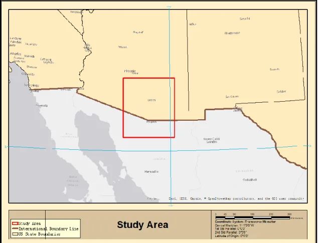
On the basis of the method chosen to downscale SMAP data, the regression model has multiple parameters to decide. Thus, the research area covers 42 SMAP pixels that guarantee the reliability of model building. To validate the final downscaling results, SMAPVEX 15 field observation are compared and calculated. Considering all the requirements, the study area of 42 SMAP level pixels are shown as figure 3.1. The time period of the study in this region is match SMAPVEX 15 validation program.
The study area covers an area over 74,000 square kilometers and it locates in southwest United States. To be specific, 42 SMAP-level pixels are taken as the research region. Parts of Arizona and Mexico are included. This area also includes validation sites of SMAPVEX15 program. As both Arizona, US and Mexico are known for its desert view and the arid climate, it is obvious that the annual rainfall in this area is relatively low. In addition, Soil types in this region are mostly gravel and sand which have good capability of drainage.
For the dataset of SMAPVEX 15, the data collected in the region called Walnut Gulch Experimental Watershed (WGEW) which located in southeast Arizona. Operated by the USDA, the Walnut Watershed covers a semi-arid area around 148 square km. The average annual temperature in the region is around 17.7°C. Within the range of observation sites, most of the surface area is covered with shrub and grass (97%), the other areas are defined as developed open space (2%). The semiarid climate brings more than half of the precipitation during summer from July to September, annual precipitation around 350 mm. In the study time period around August, North American monsoon (NAM) influence the study area and brings intense but brief thunderstorms. Such a heavy rainfall will obviously affect the local ecosystem and the balance of
14
all the contents in soil (Moran et al., 2015). This area is perfect for validation of soil moisture because of these climate change events result in. The shifting precipitation provides more informative samples for the study.
15
16
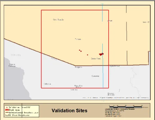
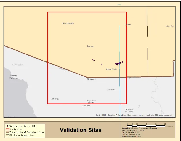
Figure 3.3. Validation Sites 08-13 (23 stations)
3.2. Datasets
3.2.1. SMAP Level 3 products
NASA launched the Soil Moisture Active Passive (SMAP) mission in January 2015 and it has been serving as an important global soil moisture observation mission since then. SMAP carries both radar and radiometer instruments which designed to detect soil moisture and recognize the freeze or thaw state of the mapping area. The observation of soil moisture level focus on the top 5 cm of surface, mapped by both radar and radiometer measurements. The radar instruments are in charge of ‘Active’ by transmitting pulses of radio waves down to the Earth’s
17
surface and analyze the returning echo. The radiometry instrument, on the other hand, stands for ‘passive’, as it detects radio waves emitted by the ground and measures the temperature.
The project’s antenna covers a swath of 1000 km wide on the ground that completed soil moisture maps of Earth every 2 to 3 days. The SMAP mission generate all 15 data products and eventually represent 4 levels of data processing. As to the soil moisture products, there are three types of data, each stand for active(radar), passive(radiometer), active and passive (radar + radiometer) microwave data. The data product has the resolution of 3 km, 36 km and 9 km. In this thesis, we are using the Level 3 SMAP data (SPL3SMP). The Level 3 data product use the input L-band brightness temperature level to produce soil moisture data. This level also has the only freeze/thaw product in the SMAP mission. The product provides surface soil moisture in m3/m3. In this study, the 36-km resolution level 3 data is used for downscaling research collected
from National Snow & Ice Data Center (https://nsidc.org/). In the data processing procedure, it is shown at 40-km resolution output on a fixed Earth-2 projection (Knipper et al., 2017). The product contains two set of soil moisture collected from Local Solar Time (LST) 6 am or 6 pm. Considering the collection time of 6 am is close to the NDVI data, 6 am product is utilized (around 10:30 am).
3.2.2. MODIS products
NASA launched the Terra mission (formerly known as EOS AM-1) in December, 1999 and had the Aqua mission (EOS PM-1) launched in May, 2002. These satellites have two
different orbits that one runs north to south, vertical to the equator, and the other one passes from south to north. The combination of the 36 spectral bands from Terra and Aqua mission turns into the Moderate Resolution Imaging Spectroradiometer (MODIS). It is a global observation with a frequency around 1 to 2 days. The MODIS instruments provide the atmospheric, land and ocean
18
images to all users. In this study, the version 6 MODIS aqua daily day time LST product (MOD11A1), MODIS terra/aqua 16-day composite Normalized Difference Vegetation Index (NDVI) is used as variables to build the downscaling model for estimate soil moisture. These datasets have the spatial resolution around 1 km.
The 1-km resolution daily LST product (MOD11A1) provides per-pixel land surface temperature data that derived from level 2 swath products. Giving consideration of overlapping observations, average LST values from all qualify observations are taken in this circumstance. This product gets rid of the interference of cloud from level 3 and level 2 products.
Improvements are also made on the split-window algorithm and adjusting weights in the day/night algorithm ("MOD11A1 V006 | LP DAAC :: NASA Land Data Products And Services").
The MOD13A2 1-km product not only provides two Vegetation layers, but also includes two Quality Assurance (QA) layers and Reflectance bands as well as four observation layers. The MOD13A2 version 6 product pick the best available value from all the pixel values obtained in the 16-day period. Only the highest NDVI value with low cloud and low view angle will be up to the standard. Among all these indexes, NDVI is utilized in the model building. Both NDVI composite product are generated by two 8-day Surface Reflectance product ("MOD13A2 V006 | LP DAAC :: NASA Land Data Products And Services").
For downscaling purpose, NDVI as primary vegetation index is chosen. NDVI calculates vegetation index within a value range between -1 to 1 based on a simple equation as in Equation 1 and is the most widely used vegetation index tested with various studies.
nir red nir red R R NDVI R + R − = ,(1)
19
Where Rnir and Rred represent the reflectance values of the red and NIR bands
respectively.All MODIS products are acquired from the NASA Atmosphere Archive & Distribution System (LAADS) Distributed Active Archive Center (DAAC) site
(https://ladsweb.modaps.eosdis.nasa.gov/) in the standard hierarchical data format for the time period under investigation. Before model building, all remote sensing images are projected to WGS 1984 17 N system.
3.2.3. SRTM 1 arc-second product
The Shuttle Radar Topography Mission (SRTM) was launched by National Aeronautics and Space Administration (NASA) and National Imagery and Mapping Agency (NIMA) on February 2000. This joint mission is aimed to collect topographic data for most of the land surface over the globe. The mission use radar interferometry to achieve surface elevation. Transmitting the radar wave to the earth’s surface, the scatter waves received by main antenna and outboard antenna came back with differences. Known the accurate baseline distance between the main antenna and outboard antenna, the land surface elevation can be calculated. The spatial resolution for SRTM products is 1 arc-second (around 30 meters) and 3 arc-second (around 90 meters). In the thesis, SRTM 1 arc-second global elevation data is used.
3.2.4. SMAPVEX15 observation
The SMAPVEX program is a validation experiment that is developed to assess the accuracy of SMAP data. The first experiment was conducted in 2012. SMAPVEX-15 was carried out in southern Arizona, United States. To create a more spatially and temporally complex experimental environment, the experiment is proceeded during Summer Monsoon. Some certain dates in August that data from other satellites providing soil moisture estimates are available in this region. Both network stations and airborne sensors come into service. For
20
aircraft component, Passive Active L-band System (PALS), the Uninhabited Aerial Vehicle Synthetic Aperture Radar (UAVSAR), and Airborne Microwave Observatory of Subcanopy and Subsurface (AirMOSS) are utilized in this experiment. Among the three components, PALS is the key method in SMAPVEX15 ("SMAP: SMAPVEX15").
Most of the SMAPVEX 15 data is collected by distributed soil moisture network
composed by nearly 80 stations. The ground-based sampling mainly uses Stevens Hydra Probes which installed underground 5 cm to get the effective soil moisture. Measurements of soil moisture is averaged between 5:00 a.m. and 7:00 a.m. to match satellite overpass times. The SMAPVEX 15 data also downloaded from National Snow & Ice Data Center (https://nsidc.org/).
The Volumetric Soil Moisture (VSM) used in the validation is probe-reading data. To match with the retrieval footprint of SMAP products, the field station utilized multiple sample sites which meets statistical criteria. The scale of field observation data is 800 m that close to the downscaled result. Unit for the ground soil moisture is m3/ m3 which is the same with original SMAP soil moisture retrieval.
21
CHAPTER 4. METHODS
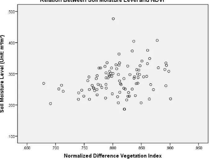
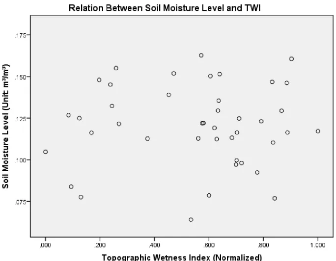
The following scatter plots demonstrate the relation between soil water level and the variables. All the docs represent the mean value of indexes from the 100-pixel research area. Soil moisture level as the Y-axis and variables in the model serve as the X-axis. All data value is being normalized for intuitive view before generating scatter plot. Based on the scatter plots, distribution of NDVI can be conclude by linear relation, while both LST, DEM and TWI do not show strong linear relation to soil moisture value. Thus, nonlinear regression model is adopted for this thesis research.
22
23
24
Figure 4.4. Scatter Plot of TWI and Soil Moisture
4.1. Multiple regression model 4.1.1. Model 1
As stated above, multiple regression method has many advantages for soil moisture downscaling. In this research, two regression models are used. NDVI and LST serve as two independent variables. DEM data is added to equation 7 as the second model. According to the requirements of the multiple regression model, the variable assumed to be the independent variable which leads to affecting soil moisture. Piles (2011) indicate that soil moisture, LST,
25
vegetation index has multivariate nonlinear regression relationship and can be calculated by Equation 3. The formula stated as follow:
* * 0 0 SM= NDVI LST , j n i n i j ij i j a = = = =
(2)The formula is interpretate to the following equation:
00 01 10 11
SM=a +a *LST+a * NDVI+a * NDVI*LST, (3)
n is the order of the model, aij represents the regression coefficients of the independent
variable.SM stands for soil moisture estimates, while LST* represents the normalized observed LST. For better performance of the regression model, normalization process is conduct to all datasets. Specific definition is as follows,
* min max min LST - LST LST , LST - LST = (4)
LSTmin and LSTmax represent the minimum and maximum LST values in the research
area.
4.1.2. Model 2
To achieve better downscaled results, elevation value is introduced to the model. The second model work as a nonlinear regression model and the equation is as follows,
* * * 0 0 0 SM = NDVI LST DEM n n n i j k ijk i j k a = = =
, (5)The equation can be defined as follows,
000 100 010 001 110
2 2 2
101 011 200 020 002
SM * NDVI + * LST + * DEM + * NDVI * LST
+ NDVI * DEM + LST * DEM + * NDVI + * LST + * DEM
a a a a a
a a a a a
= +
, (6)
To entirely interpret Equation 7, 27 parameters along with multiple variables overlay with each other in many polynomials. To avoid similar polynomials interfering the model
26
building, all polynomials contain more than 2 variables are removed. Research in 2014 also indicated the reliability of this formula interpretation (Piles et al., 2014). Normalization is also executed before regression process. The method of normalization is the same as shown in the equation 4.
4.1.3. Model 3
Topographic Wetness Index (Sorensen et al. 2007) is a steady-state wetness index computed from the high-resolution DEM models. It assumes the soil water content (wetness) distribution is controlled by the two factors: contributing area (a) and the local slope. The equation is written as:
TWI = ln(a/s), (7)
TWI was calculated from the 30 m resolution DEM obtained from the USGS National Elevation Dataset (NED). The data was originally provided in the Geographic Coordinate System at the 1/3 arc-second resolution (approximated 30 m). The DEM was mosaicked and projected to the UTM 12 N coordinate system and clipped to fit the extend of the SMAP data. A TWI model was created in ArcGIS to derive TWI using a string of functions including “fill depression”, “flow accumulation”, and “slope”. The graphic view of the TWI model was shown in the following figure.
* * * 0 0 0 SM = NDVI LST TWI n n n i j k ijk i j k a = = =
, (8)The equation above is interpreted into the following:
000 100 010 001 110
2 2 2
101 011 200 020 002
SM * NDVI + * LST + * TWI+ * NDVI * LST
+ NDVI * TWI + LST * TWI + * NDVI + * LST + * TWI
a a a a a
a a a a a
= +
27
There are 10 parameters in the equation. To entirely explain the original formula, there will be much more parameters than 10. But for the same reason as it is explained in previous section, all polynomials contain more than 2 variables are eliminated in order to reduce interferences between variables. In the research, second-order polynomial regression model is applied in model building process for computational efficiency. SPSS is employed for analyzing the dataset and generate the regression models.
4.2. Downscaling methodology
In general, the downscaling method in this paper assumes the coefficient of model parameters would not change with the scale. The low-resolution images are utilized to generate the regression model, then the model is applied with the high-resolution image to achieve
downscaled high-resolution soil moisture data. The entire route of the experiment is divided into few steps, reprojection, resample, normalization and regression. Modeling results are validated with field observation from two separate dates. Several studies have shown the strong correlation between soil moisture, LST, vegetation index, DEM and TWI. To downscale the low-resolution data, SMAP images and supplemental data are utilized to calculate the regression model and further produce detailed soil moisture maps.
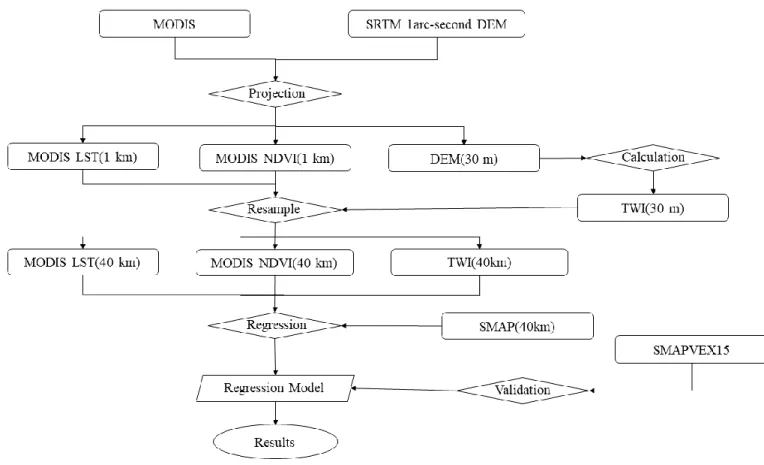
4.3. Route of technology
The entire route of technology for this thesis is shown in figure 4.1. It addresses the all the necessary datasets and research methods used in the practice. On the basis of using second-order polynomial regression model, 9 coefficients would be generated, which requires at least 10 pixels to be the input dataset. To meet the requirement, a 6*7 cell research area is chosen in the study. 100 pixels of the SMAP data are downscaled with 1-km MODIS products and 30-m SRTM elevation image in the same area same time period.
28
For the preprocess procedure, original 1-km spatial resolution MODIS are projected to WGS 1984 (17N) in ENVI. The 30-m resolution DEM images are also projected to the same projection system. Resampling procedure is conducted by calculating the mean of all the vegetation index value, LST values and elevation within the larger pixel (40 km ×40 km), the MODIS 1-km resolution data is aggregated to 40-km scale. For regression model, three models are utilized by different variables for comparison. The first model takes LST and NDVI image as high-resolution input, the second model prefers LST, NDVI and DEM while the third model process LST, NDVI and TWI data instead. High-resolution soil moisture level is computed based on the regression formula. After the preprocess and model building, SMAP data is downscaled using the regression models stated above. The final step is to validate the downscaling output with the SMAPVEX15 field observation. Results from three regression models are compared with the field data of two different dates. To evaluate the regression model, not only the
comparison results are being assessed, but also the fitting degree of the model simulation and the in-situ data.
29
30
31
32
CHAPTER 5. RESULTS AND DISCUSSION 5.1. Data analysis
Considering the validation data SMAPVEX 15 is conducted during August 2nd to August 18th, datasets from the same time period are picked for the validation, but after evaluating the LST images in the validation region, only August 2nd and August 13th MODIS images provide available LST value without missing too much area with cloud cover. The models are built based on 42-pixels research area and the regression models are validated by the field observation in Arizona. The NDVI/ LST/ DEM/TWI condition of research area in Arizona is demonstrated in Figure 5.1. It is obvious that the mountain in the study region not only affect elevation, but the vegetation cover and land surface temperature appear the same pattern. As the elevation increase, vegetation cover decreases while the surface temperature drops. In the validation area, the
33
34
Figure 5.2. Land Surface Temperature of Study Area (a) 08-02 LST; (b) 08-13 LST
5.2. Modeling results for Model 1
After image processing, downscaling model based on NDVI and LST is generated. With calculating the original SMAP 40-km soil moisture, parameter estimates of variables provide the relation between variables and soil moisture level. The downscaled results of the study area are achieved by applying the model on MODIS-level resolution data.
35
The coefficient of parameters for Model 1 experiments are listed as Table 5.1 and 5.3. Each table represent the data from each experiment date. The correlation of estimated parameters is shown in table 5.2 and 5.4. The correlation of parameter estimates illustrates each variable are strongly correlated to each other. However, Model 1 is a nonlinear regression, in that case, the law of correlation is not suitable for this situation. In common cases, high correlation of each parameter requires further examination of multicollinearity. However, given the condition of nonlinear regression, there is no need for multicollinearity test. Also, for the same reason of nonlinear regression, the ANOVA table with R square does not represent the fitting degree of the model. In this research, validation results show the accuracy and the fitting degree of the
regression model. All three models are evaluated by calculating the mean absolute error (MAE) and root mean square error (RMSE).
Table 5.3. Model 1 parameter estimation of soil moisture in 08-02
Parameter Estimates
Parameter Estimate Std. Error
95% Confidence Interval Lower Bound Upper Bound
a00 .115 .025 .063 .167
a01 .020 .034 -.049 .089
a10 -.002 .053 -.109 .106
a11 -.027 .099 -.228 .174
Table 5.4. Correlation of parameter estimates in 08-02
Correlations of Parameter Estimates
a00 a01 a10 a11
a00 1.000 -.895 -.917 .521
a01 -.895 1.000 .900 -.789
a10 -.917 .900 1.000 -.741
36
Table 5.5. Model 1 parameter estimation of soil moisture in 08-13
Parameter Estimates
Parameter Estimate Std. Error
95% Confidence Interval Lower Bound Upper Bound a00 .115 .025 .063 .167 a01 .020 .034 -.049 .089 a10 -.002 .053 -.109 .106 a11 -.027 .099 -.228 .174
Table 5.6. Correlation of parameter estimates in 08-13
Correlations of Parameter Estimates
a00 a01 a10 a11 a00 1.000 -.895 -.917 .521 a01 -.895 1.000 .900 -.789 a10 -.917 .900 1.000 -.741 a11 .521 -.789 -.741 1.000
37
Corresponding downscaled soil moisture product also listed as figure 5.4 and figure 5.5. The comparison result is quite clear in the downscaled product here. If the conclusion were only made based on the low-resolution data, we are only able to presume that the northwest pixel has the lowest moisture level while the southeast has the lowest. But more detailed information is provided with the downscaled remote sensing image. The overall downscaled image fits the terrain character of the study region. Pattern of soil moisture level matches the local topography. The blank space in the image is caused by the missing LST value. Missing LST value is one of the biggest problems in the process. There are many reasons for causing the problem, cloud is the most common cause, which is quite normal during the summer monsoon.
38
Figure 5.8. Left: 08-13 SMAP image; Right: Downscaled SMAP data (Model 1)
5.2. Modeling results for Model 2
The following Table 5.2 represents the parameter estimates for Model 2. Correlation of each parameter estimates are also high. Same with previous modeling result, the high correlation between each parameter are reasonable because of the nonlinear regression.
39
Table 5.9. Model 2 Estimation of Soil Moisture (08-02)
Parameter Estimates
Parameter Estimate Std. Error
95% Confidence Interval Lower Bound Upper Bound
a000 .102 .071 -.043 .247 a100 -.284 .245 -.784 .217 a010 .059 .152 -.251 .368 a001 .222 .137 -.057 .501 a110 .160 .189 -.225 .544 a101 .272 .227 -.191 .734 a011 -.158 .131 -.426 .110 a200 .024 .310 -.608 .657 a020 -.022 .090 -.206 .161 a002 -.189 .090 -.372 -.006
Table 5.10. Correlation of Parameter Estimates for Model 2 (08-02)
Correlations of Parameter Estimates
a000 a100 a010 a001 a110 a101 a011 a200 a020 a002 a000 1.000 -.724 -.897 -.473 .697 .142 .512 .456 .768 .345 a100 -.724 1.000 .484 -.134 -.787 .269 .069 -.872 -.338 -.193 a010 -.897 .484 1.000 .456 -.661 -.184 -.533 -.211 -.964 -.249 a001 -.473 -.134 .456 1.000 .126 -.517 -.916 .268 -.400 -.488 a110 .697 -.787 -.661 .126 1.000 -.092 -.154 .523 .555 .041 a101 .142 .269 -.184 -.517 -.092 1.000 .411 -.653 .156 -.461 a011 .512 .069 -.533 -.916 -.154 .411 1.000 -.160 .503 .441 a200 .456 -.872 -.211 .268 .523 -.653 -.160 1.000 .110 .407 a020 .768 -.338 -.964 -.400 .555 .156 .503 .110 1.000 .202 a002 .345 -.193 -.249 -.488 .041 -.461 .441 .407 .202 1.000
40
Table 5.11. Model 2 Estimation of Soil Moisture (08-13)
Parameter Estimates
Parameter Estimate Std. Error
95% Confidence Interval Lower Bound Upper Bound a000 .102 .071 -.043 .247 a100 -.284 .245 -.784 .217 a010 .059 .152 -.251 .368 a001 .222 .137 -.057 .501 a110 .160 .189 -.225 .544 a101 .272 .227 -.191 .734 a011 -.158 .131 -.426 .110 a200 .024 .310 -.608 .657 a020 -.022 .090 -.206 .161 a002 -.189 .090 -.372 -.006
Table 5.12. Correlation of Parameter Estimates for Model 2 (08-02)
Correlations of Parameter Estimates
a000 a100 a010 a001 a110 a101 a011 a200 a020 a002 a000 1.000 -.724 -.897 -.473 .697 .142 .512 .456 .768 .345 a100 -.724 1.000 .484 -.134 -.787 .269 .069 -.872 -.338 -.193 a010 -.897 .484 1.000 .456 -.661 -.184 -.533 -.211 -.964 -.249 a001 -.473 -.134 .456 1.000 .126 -.517 -.916 .268 -.400 -.488 a110 .697 -.787 -.661 .126 1.000 -.092 -.154 .523 .555 .041 a101 .142 .269 -.184 -.517 -.092 1.000 .411 -.653 .156 -.461 a011 .512 .069 -.533 -.916 -.154 .411 1.000 -.160 .503 .441 a200 .456 -.872 -.211 .268 .523 -.653 -.160 1.000 .110 .407 a020 .768 -.338 -.964 -.400 .555 .156 .503 .110 1.000 .202 a002 .345 -.193 -.249 -.488 .041 -.461 .441 .407 .202 1.000
Figure 5.13 and 5.14 is the downscaled SMAP data of research area. The image shows that DEM result distribution is different from the original SMAP image. Using the same classification of DEM-derived modeling result, the SMAP image does not provide any detail
41
information especially about the southeast corner. The entire distribution apparently match with the actual SMAP distribution of moisture level. Fitting degree of Model 2 will be examined later in the validation.
42
Figure 5.14. Left: 08-13 SMAP image; Right: Downscaled SMAP data (Model 2)
5.3. Modeling results for Model 3
The parameter estimates of model 3 for August 2nd, 2015 are listed in the following Table 5.5 while Table 5.6 shows the correlation of parameter estimates. The comparison of the original SMAP soil moisture data and the model-based downscaled soil moisture image can be reached in
43
figure 5.8. The downscaled image is aggregated to the MODIS level pixel size, which is also showing the same pattern with the original SMAP data. The blank region in the image is caused by the missing data of surface temperature. Cloud and climate are the main reason for the missing area. The downscaled soil moisture map provided more precise image than the SMAP data. For example, SMAP products are not able distinct the difference of soil water level between pixels, while the downscaled map provided detail information especially for the southeast side of the study area.
Table 5.15. Model 3 estimation of soil moisture in 08-02
Parameter Estimates
Parameter Estimate Std. Error
95% Confidence Interval Lower Bound Upper Bound
a000 .311 .131 .045 .578 a100 -.621 .421 -1.480 .238 a010 .017 .187 -.364 .399 a001 -.342 .167 -.683 -.001 a110 -.008 .257 -.532 .517 a101 .563 .233 .087 1.038 a011 .093 .118 -.147 .333 a200 .455 .364 -.287 1.196 a020 -.030 .094 -.222 .162 a002 .073 .088 -.107 .253
44
Table 5.16. Model 3 correlations of parameter estimates in 08-02
Correlations of Parameter Estimates
a000 a100 a010 a001 a110 a101 a011 a200 a020 a002 a000 1.000 -.947 -.735 -.776 .771 .805 .633 .837 .388 .296 a100 -.947 1.000 .612 .693 -.740 -.770 -.535 -.965 -.260 -.256 a010 -.735 .612 1.000 .264 -.924 -.306 -.543 -.477 -.819 .114 a001 -.776 .693 .264 1.000 -.290 -.932 -.508 -.578 .021 -.659 a110 .771 -.740 -.924 -.290 1.000 .347 .489 .647 .675 -.052 a101 .805 -.770 -.306 -.932 .347 1.000 .595 .670 -.019 .429 a011 .633 -.535 -.543 -.508 .489 .595 1.000 .430 .039 -.243 a200 .837 -.965 -.477 -.578 .647 .670 .430 1.000 .147 .210 a020 .388 -.260 -.819 .021 .675 -.019 .039 .147 1.000 -.039 a002 .296 -.256 .114 -.659 -.052 .429 -.243 .210 -.039 1.000
Table 5.17. Model 3 estimation of soil moisture in 08-13
Parameter Estimates
Parameter Estimate Std. Error
95% Confidence Interval Lower Bound Upper Bound a000 .311 .131 .045 .578 a100 -.621 .421 -1.480 .238 a010 .017 .187 -.364 .399 a001 -.342 .167 -.683 -.001 a110 -.008 .257 -.532 .517 a101 .563 .233 .087 1.038 a011 .093 .118 -.147 .333 a200 .455 .364 -.287 1.196 a020 -.030 .094 -.222 .162 a002 .073 .088 -.107 .253
45
Table 5.18. Model 3 correlations of parameter estimates in 08-13
Correlations of Parameter Estimates
a000 a100 a010 a001 a110 a101 a011 a200 a020 a002 a000 1.000 -.947 -.735 -.776 .771 .805 .633 .837 .388 .296 a100 -.947 1.000 .612 .693 -.740 -.770 -.535 -.965 -.260 -.256 a010 -.735 .612 1.000 .264 -.924 -.306 -.543 -.477 -.819 .114 a001 -.776 .693 .264 1.000 -.290 -.932 -.508 -.578 .021 -.659 a110 .771 -.740 -.924 -.290 1.000 .347 .489 .647 .675 -.052 a101 .805 -.770 -.306 -.932 .347 1.000 .595 .670 -.019 .429 a011 .633 -.535 -.543 -.508 .489 .595 1.000 .430 .039 -.243 a200 .837 -.965 -.477 -.578 .647 .670 .430 1.000 .147 .210 a020 .388 -.260 -.819 .021 .675 -.019 .039 .147 1.000 -.039 a002 .296 -.256 .114 -.659 -.052 .429 -.243 .210 -.039 1.000
46
47
Figure 5.20. Left: 08-13 SMAP image; Right: Downscaled SMAP data (Model 3) Considering the two downscaled maps, some information of the model performance is clear. The spatial pattern of downscaled results matches the original SMAP data. Both maps indicate that the southeast part of study area tends to be drier and more arid than the other part of the area. Placing the Model 2 results with Model 3 results, the Model 3 results provide a finer grain than Model 2. DEM-derived model has a smoother image than TWI-based one. During the calculation of TWI, contribution area and local slope are taken into consideration, which can explain the granular sensation of Model 3 soil moisture maps.
48
5.4. Validation Results
After producing downscaled maps, all results are combined with SMAPVEX 15 data for validation. To evaluate the results, 22 ground observation of soil moisture data are chosen as ground truth value. MAE (Mean Absolute Error) of SMAP data and three downscaled methods are calculated as Table 5.5. Unlike ME (Mean Error), MAE avoid additional errors caused by the cancellation of positives and negatives. MAE is a common measurement of the differences between two groups of variables. It compares the prediction value with the observation. As present in the table, downscaled results have lower MAE than the original SMAP data, indicating the feasibility of the regression model.
Table 5.21. Mean Absolute Error Comparison
MAE Model 1 Model 2 Model 3 SMAP
08-02 0.042835 0.092580 0.052023 0.261907
08-13 0.031265 0.031011 0.032850 0.158449
RMSE, known as root-mean-square deviation or root-mean-square error, is a common measurement of fitting degree of regression model. RMSE measures the average magnitude error between predicted value and observation value, so it is regarded as model’s capability of
prediction. In Table 5.6, RMSE of all models’ performance in validation are calculated and compared.
Table 5.22. Root Mean Square Error of Each Models
RMSE Model 1 Model 2 Model 3 SMAP
08-02 0.049016 0.101159 0.062727 0.067731
49
Since the errors are squared before they are divided, RMSE reveals the condition when there are large errors in the dataset. Base on the mean absolute error, the original SMAP image has larger errors in general compared with the downscaled results. It is obvious that the
regression models perform better than the original SMAP images, especially Model 1 and 3. Given the differences of MAE and RMSE, statistics show that there is no large outlier in the errors of downscaled soil moisture level.
Comparing results from SMAP data and downscaled soil moisture images, all three models perform better than the original SMAP data. Given the condition of models derived by two factors and three factors, Model 2 (DEM-derived) do not serve as satisfactory in
experiments. Meanwhile, Model 3 do not enhance the performance either. Introducing the Topographic Wetness Index to the model bring better consistency and fitting than elevation-derived model. Both MAE and RMSE of TWI-elevation-derived model is smaller than the DEM-elevation-derived model, suggesting better execution in downscaling. As result, it indicates Model 3 performs relatively better than Model 2. However, the TWI-based model results show slight difference with Model 1. Instead of profound improvement, TWI provide a similar outcome comparing to Model 1.
5.4.1. Validation Result of 08-02-2015
Model-generated soil moisture maps are compared with the original SMAP images. The downscaled results indicating the unsatisfying performance of Model 2. DEM-based model does not show any advantage in the downscaling. Model 2 results in much higher moisture level not only compared to the original SMAP value, but also to the in-situ data. Meanwhile, Model 1 and Model 3 perform decently and produce detailed downscaled results. Both the maps generated by Model 1 and Model 3 appear the same pattern, which match with the local LST and TWI images.
50
Chart 5.23. Validation data and Model Estimates (08-02)
Chart 5.24. Absolute Error of Each Model Estimates (08-02) 0.00 0.02 0.04 0.06 0.08 0.10 0.12 0.14 0.16 0.18 0 5 10 15 20 25 Soi l M oistu re L eve l( m 3/m 3)
Serial Number of Observation Station
Absolute Error of Each Model Estimates 08-02
Error_smap Error_m1 Error_m2 Error_m3 0.00 0.05 0.10 0.15 0.20 0.25 0 5 10 15 20 25 Soi l M oistu re L eve l( m 3/m 3)
Serial Number of Observation Station
Validation data and Model Estimates 08-02
51
These two charts are the absolute error between model-predicted value and the actual field observation. All three model results and the original SMAP data are compared with the validation data. Base on the charts above, it is obvious that all three model has the approximate error in predicting soil moisture level. Comparing the modeling results from SMAP data, it can conclude that the models are more precise than the original SMAP data. These downscaled maps fit the spatial pattern of elevation or surface temperature.
5.4.2. Validation Result of 08-13-2015
The following figure is Model-generated soil moisture maps compared with the original SMAP images. Model 1 results have relatively small RMSE, which indicating a good fitting of the model. The results support the statement that Model 1 in this study is valuable in soil moisture estimation. In term of the accuracy of predicted result, the downscaled results from three models are in the same level in 08-13 experiment. Comparing the MAE and RMSE of Model 1 and Model 3, they have very much the same MAE but the difference in RMSE is greater, indicating Model 2 has greater errors than Model 1.
52
Chart 5.25. Validation data and Model Estimates (08-13)
Chart 5.26. Absolute Error of Each Model Estimates (08-13) 0.00 0.02 0.04 0.06 0.08 0.10 0.12 0.14 0 5 10 15 20 25 Soi l M oistu re L eve l( m 3/m 3)
Serial Number of Observation Station
Absolute Error of Each Model Estimates 08-13
Error_smap Error_m1 Error_m2 Error_m3 0.00 0.05 0.10 0.15 0.20 0.25 0 5 10 15 20 25 Soi l M oistu re L eve l( m 3/m 3)
Serial Number of Observation Station
Validation Data and Model Estimates 08-13
53
5.5. Discussion
Model 2 and 3 are designed to test out the performance of two variables, DEM and TWI. Base on previous research and results from Model 1, surface temperature and vegetation index are proved to be spatial correlated to soil moisture. The experiments are established based on the idea that bring a new factor to the regression model will bring stability and better outcome. Adding the elevation value and wetness index to linking model, the downscaling results are not significantly improved comparing to the Model 1 results. According to the current outcome, TWI-derived model outperforms the DEM model. The result suggests that DEM is not profound correlate to moisture level as it is expected to be. DEM- derived model has an RMSE that is remarkable higher than the other two modeling results. A high value RMSE is not acceptable because the moisture level itself is usually small in the study area.
In order to achieve ideal outcome, TWI is calculated and put into service in the third experiment. The Topographic Wetness Index (TWI), also called Compound Topographic Index (CTI), is an index that represents the topographic character of the terrain. By calculating the flow accumulation and slope, TWI is a steady index for soil moisture estimation. Model 3 results meet the expectation of high accuracy estimation. Compared with ground observation, the RMSE from two separate validation dates are relatively small. RMSE rang from 0.04 to 0.07, suggest the reliable stability of Model 3. Given the consideration of soil water level in the validation area is within 0.4 m³/m³, RMSE of 0.04 indicating the high accuracy of the downscaled results.
However, the overall outcome of the TWI-based model does not show strong
improvement comparing to Model 1. Both MAE and RMSE of the validation indicates TWI does not prominently enhance the modeling performance. Based on the characteristic of TWI, the possible reasons of the inadequate results are as follows.
54
TWI is very sensitive to the grid size of original DEM. It is reasonable soil moisture could be affected by small scale topography. Slope smaller than the pixel size (30 m) may not be captured by the sensor which might have profound influence on the final modeling results. With more accurate TWI data, might achieved more solid downscaling result.
In the experiments, considering the limitation of data acquisition, LST is a daily data that may be more temporally relate to soil moisture level. For comparison, TWI is derived from SRTM 1 arc-second data which is collected on February 2000. The topography of the research area may have some changes that did not presented by the TWI image.
In other studies, researchers also indicate the topographic wetness index is not strongly correlated to surface soil moisture. Sanchez tested the effect of critical factors on soil moisture. Factors, such as topography and land use, did not show clear spatial correlation with soil moisture. Meanwhile, distribution of precipitation had a remarkable relation to soil moisture (Sanchez et al., 2012).
Based on the results of this study, further research on regression model is emphasis on a few aspects. First, even though TWI and DEM do not enhance the modeling result in this experiment, TWI calculated by higher resolution elevation data may provide more accurate result. Also, new calculation method of TWI may present difference in the downscaling process. Second, daily information, for example, surface temperature is the strongest indicator in the linking model, so it is reasonable to test other daily data in the regression model. Factors, such as precipitation and freeze/thaw information, control the spatial or temporal changes of soil
moisture. Introducing new daily remote sensing data may have positive effect on the
downscaling outcome. Third, it is also important to measure the model’s stability. In order to have a more comprehensive understanding of the modeling result, it’s necessary to conduct time
55
series examination. Multiple dates from different seasons throughout the year would be ideal for the examination.
56
CHAPTER 6. SUMMARY AND CONCLUSION
In summary, the regression relationship between several important indicators and soil moisture are investigated before planning the experiments. With the knowledge of those factors, three regression models are built to downscale the SMAP level 3 products. All three models are nonlinear regression model. The results of the models have good fitting with the SMAP soil moisture.
After the models are established, and implement with high resolution MODIS image, the original SMAP 36-km resolution product is downscaled to MODIS-level 1 km resolution. The downscaled soil moisture map showed relatively better accuracy. In this study, DEM was not the strong indicator of soil moisture level as expected. Rather than simply use elevation value, TWI is calculated by measuring the accumulated area and local slope, which did not show significant efficiency in assessing soil water either.
The limitation of this research includes missing LST data caused by cloud coverage and the fixed elevation information that retrieved years before the experiment date. Further study will emphasis on the improvement of the regression model. Research direction will focus on
exanimating the pattern of the spatial correlation between other factors and soil moisture retrieval. Furthermore, using data from multiple days throughout the year to test the factors. Related research on the model’s performance with different soil type, climate or land cover is also a key point.
In general, this research has concluded the following:
1. Successfully building regression model based on surface temperature, vegetation index, elevation, wetness index and soil moisture in southwest United States.
57
2. Based on the modeling results from low resolution data, calculated downscaled soil moisture value and validated with field observation.
3.The multivariate regression model of Model 1 (NDVI and LST-based) has good fitting results. Validation confirm the fact that TWI outperform the DEM-derived model. This
downscaling method with vegetation index and surface temperature achieves better spatial resolution and lower error at same time.
4. Future study will focus on the improvement of soil moisture estimation. The time-series examination of other key factors in downscaling soil moisture is the primary goal. Repeated experiments on different soil types, vegetation cover and climates are also a direction of research.