Metric Learning for Structured Data

M E T R I C L E A R N I N G F O R

S T R U C T U R E D D ATA

B E N J A M I N PA A SS E N

Bielefeld University

,

Faculty of Technology

,

Machine Learning Research Group

s u p e r v i s e d b y

r e v i e w e d b y

m ay

10

t h

, 2019

This work would not not have been possible without help from many people, both within and beyond the work group. First and foremost, I wish to thank my supervisor, Barbara Hammer, who has been a tremendous inspiration and role model throughout my time in Bielefeld. Additionally, my reviewers, Alessandro Sperduti and Lars Schmidt-Thieme, deserve thanks for their careful and in-depth reading as well as very helpful comments for this revised version of the manuscript.

I also extend my thanks to all my co-workers, especially Bassam Mokbel, who has been a brilliant and kind mentor, Alexander Schulz, who has supported and shared my passion for prosthetic research beyond our own regular projects, and Christina Göpfert, whose sharp mind has enabled all of our shared projects.

Beyond that I owe gratitude to all my collaborators, who have kindly contributed their skill, knowledge, and time to this research, namely Sebastian Groß and Niels Pinkwart at the Humboldt-University of Berlin, Thomas Price and Tiffany Barnes at the North Carolina State University, Thekla Morgenroth at the University of Exeter, Michelle Statemeyer at the University of Melbourne, Cosima Prahm at the Medical University of Vienna, Janne Hahne at the Medical University of Göttingen, and Claudio Gallicchio as well as Alessio Micheli at the University of Pisa.

I also wish to thank my parents for their patience, trust, and support over all these years, my brother for putting up with me, my many on-line and off-line friends for their kind support and believing in me beyond reasonable degrees of confidence, especially Thekla for being both an inspiring example and challenging competition like an ideal big sibling should be, and finally my partner, who has helped me up and kept me grounded whenever needed and who has taught me a strong will, a sharp wit, and a kind heart when interacting with the world.

Finally, I would be remiss to thank the German Research Foundation who have supported this research in the project “Learning Dynamic Feedback for Intelligent Tutoring Systems” (DynaFIT, grant number HA 2719/6-2), and the center of excellence “Cognitive Interaction Technology” (CITEC, grant number EXC 277).

Distance measures form a backbone of machine learning and information retrieval in many application fields such as computer vision, natural language processing, and biology. However, general-purpose distances may fail to capture semantic par-ticularities of a domain, leading to wrong inferences downstream. Motivated by such failures, the field ofmetric learninghas emerged. Metric learning is concerned with learning a distance measure from data which pulls semantically similar data closer together and pushes semantically dissimilar data further apart. Over the past decades, metric learning approaches have yielded state-of-the-art results in many applications. Unfortunately, these successes are mostly limited to vectorial data, while metric learning for structured data remains a challenge.

In this thesis, I present a metric learning scheme for a broad class of sequence edit distances which is compatible with any differentiable cost function, and a scalable, interpretable, and effective tree edit distance learning scheme, thus pushing the boundaries of metric learning for structured data.

Furthermore, I make learned distances more useful by providing a novel algo-rithm to perform time series prediction solely based on distances, a novel algoalgo-rithm to infer a structured datum from edit distances, and a novel algorithm to transfer a learned distance to a new domain using only little data and computation time.

Finally, I apply these novel algorithms to two challenging application domains. First, I support students in intelligent tutoring systems. If a student gets stuck before completing a learning task, I predict how capable students would proceed in their situation and guide the student in that direction via edit hints. Second, I use transfer learning to counteract disturbances for bionic hand prostheses to make these prostheses more robust in patients’ everyday lives.

C O N T E N T S

Contents v

1 Introduction 1

2 Background and Related Work 7

2.1 Kernels and Distances . . . 7

2.2 Kernels for Structured Data . . . 11

2.3 Edit Distances . . . 12

2.3.1 Sequence Edit Distance . . . 12

2.3.2 Algebraic Dynamic Programming . . . 14

2.3.3 Tree Edit Distance . . . 21

2.3.4 Graph Edit Distance . . . 27

2.4 Metric Learning for Edit Distances . . . 29

2.4.1 Good Edit Similarity Learning . . . 29

2.5 Learning Vector Quantization . . . 31

2.5.1 Generalized Matrix Learning Vector Quantization. . . 32

2.5.2 Labeled Gaussian Mixture Models . . . 33

2.5.3 Relational Generalized Learning Vector Quantization . . . 36

2.5.4 Median Generalized Learning Vector Quantization . . . 36

2.6 Distance-based Time Series Prediction . . . 38

3 Sequence Edit Distance Learning 43 3.1 Method . . . 44

3.2 Experiments . . . 51

3.3 Conclusion and Limitations . . . 56

4 Tree Edit Distance Learning 59 4.1 Method . . . 60

4.2 Experiments . . . 68

4.3 Conclusion . . . 73

5 Time Series Prediction for Structured Data 77 5.1 Background and Related Work . . . 79

5.2 Method . . . 81

5.3 Experiments . . . 85

5.4 Discussion and Conclusion . . . 90

6 Application to Intelligent Tutoring Systems 91 6.1 An integrated view of edit-based hint policies . . . 92

6.2 Method . . . 103

6.3 Experiments . . . 106

6.4 Conclusion . . . 113

7 Supervised Transfer Learning 115 7.1 Related Work . . . 116

7.3 Experiments . . . 124

7.4 Conclusion . . . 128

8 Application to Bionic Hand Prostheses 129 8.1 Experiments . . . 131

8.2 Conclusion . . . 137

9 Conclusions and Outlook 139 Publications in the Context of this Thesis 143 References 145 Glossary 163 Acronyms 167 A Proofs 169 A.1 Proof of Theorem 2.1 . . . 169

A.2 Proof of Theorem 2.2 . . . 171

A.3 Proof of Theorem 2.3 . . . 172

A.4 Proof of Theorem 2.4 . . . 174

A.5 Proof of Theorem 2.5 . . . 178

A.6 Proof of Theorem 2.7 . . . 189

A.7 Proof of Theorem 2.8 . . . 193

A.8 Proof of Theorem 3.1 . . . 195

A.9 Proof of Theorem 3.2 . . . 198

A.10 Proof of Theorem 3.3 . . . 200

A.11 Proof of Theorem 3.4 . . . 202

A.12 Proof of Theorem 3.5 . . . 205

A.13 Proof of Theorem 4.2 . . . 207

A.14 Proof of Theorem 4.3 . . . 228

A.15 Proof of Theorem 5.1 . . . 231

A.16 Proof of Theorem 6.2 . . . 233

A.17 Kernelized Othogonal Matching Pursuit. . . 234

1

The notion of nearness or proximity, which is objectively de-fined only for pairs of objects in physical space, tends to be carried over to very different situations where the space in which entities can be closer together or further apart is not at all evident.

— r o g e r s h e pa r d, 1962

According to foundational works in cognitive science, proximity and distance are key concepts in our understanding of the world (Gentner and Markman 1997; Hodgetts, Hahn, and Chater 2009; Medin, Goldstone, and Genter1993; Nosofsky1992; Shepard

1962; Tversky1977). For example, we estimate the properties of an individual based on our experience with similar individuals in the past (Mussweiler 2003; Eliot Smith and Zarate 1992); we form mental categories based on similarities to exemplars (Edward Smith and Medin 1981; Markman1998); and we try to transfer solutions from known problems to new but similar problems (Barnett and Ceci2002).

These cognitive behaviors have inspired various machine learning algorithms. In particular, one-nearest-neighbor or learning vector quantization classify data by assigning the label of the closest exemplar in a data base (Cover and Hart 1967; Kohonen1995), k-means or relational neural gas cluster data based on their distance to cluster means (MacQueen 1967; Hammer and Hasenfuss2007), and multiple transfer learning algo-rithms optimize the similarity between data from related domain to transfer knowledge between these domains (Duan, Xu, and I. Tsang 2012; Kulis, Saenko, and Darrell2011; Weiss, Khoshgoftaar, and D. Wang2016). Key to all these approaches is that we have a sufficient understanding of what it means for objects to be similar ordifferent (Medin, Goldstone, and Genter1993). In other words, we require a measure of distance that is reasonable for our task at hand.

In most machine learning applications, we utilize general-purpose metrics, such as the Euclidean distance (Bellet, Habrard, and Sebban 2014). However, because these metrics do not take particularities of a domain into account, they may lead to incorrect inferences. For example, when classifying the control signal for a prosthesis, some channels of the signal may be more predictive than others (Paaßen et al.2018). More generally, default metrics may fail to regard semantically similarly objects as similar because their data representation appears different, and may fail to regard semantically different objects as different, because their data representation appears similar. Therefore, any subsequent inferences based on apparent similarity or difference may be semantically flawed.

This begs the question, how can we learn a metric better takes domain-specific semantics into account? This very question is at the heart of metric learning (Bellet, Habrard, and Sebban2014; Kulis2013). Generally speaking, a metric learning approach takes as input a setN+_{of semantically close pairs(x,y)as well as a setN}−_{of semantically} distant pairs(x,y)and attempts to learn parametersΛof a metricd_Λ such thatd_Λ(x,y)

is small for all(x,y)∈ N+and d_Λ(x,y)is large for all(x,y)∈ N−(Bellet, Habrard, and Sebban2014).

Most metric learning approaches to date learn a generalization of the Euclidean distanced, namely the generalized quadratic form

d_Λ(~x,~y) = q

(~x−~y)>_{·Λ·(~x−~y)}

where ~x and~y are m-dimensional real vectors and Λ is a symmetric, positive semi-definitem×m-matrix, which constitutes the parameters to be learned (Bellet, Habrard, and Sebban2014; Kulis2013; Schneider, Biehl, and Hammer2009a). This kind of metric learning has been widely successful and has achieved state-of-the-art performance in various information retrieval tasks, especially in computer vision (Bellet, Habrard, and Sebban2014; Davis et al.2007; Köstinger et al.2012; Liao et al.2015; Lim, Lanckriet, and McFee 2013; Davis et al.2010). A key appeal is that a learned generalized Euclidean distance retains intuitive properties of the data, such as symmetry, non-negativity, shift-invariance, and the triangular inequality. Furthermore, Euclidean metric learning is flexible enough to support a broad range of cost functions, as well as various architectures and parametrizations, such as deep learning models (De Vries, Memisevic, and Courville

2016; Hu, Lu, and Tan2014; Oh Song et al.2016).

However, not all problems involving distances can be tackled with a generalized Euclidean distance. As Hodgetts, Hahn, and Chater (2009) point out: “Real-world ob-jects are not merely represented as lists of features or dimensions but represented in a structured way that considers not only the composite elements but the relations between these different elements.” Examples of suchstructured datainclude chemical processes, human and animal motion data, electrocardiography readings, financial time series, natural language sentences and syntax trees, abstract syntax trees of source code, RNA, DNA, and protein sequences, phylogenetic trees, RNA secondary structures, and glycan molecules (Akutsu2010; Bellet, Habrard, and Sebban2014; S. Henikoff and J. G. Henikoff

1992; Keogh and Ratanamahatana2005; McKenna et al.2010; Mikolov et al.2013; Pawlik and Augsten2011; Rivers and Koedinger2015; T. F. Smith and Waterman1981; Snover et al.2006). For such structured data, we requirestructure metrics, such as the Levenshtein distance, dynamic time warping, or the tree edit distance (Levenshtein1965; Vintsyuk

1968; Zhang and Shasha1989).

As with the Euclidean distance, these structure metrics may not correspond to domain-specific semantics. For example, when analyzing protein sequences, the standard string edit distance assumes that all amino acids have the same pairwise distance which does not correspond to biological reality (S. Henikoff and J. G. Henikoff1992; Hourai, Akutsu, and Akiyama 2004; Kann, Qian, and Goldstein 2000; Saigo, Vert, and Akutsu 2006). Similarly, when considering abstract syntax trees of source code, the standard tree edit distance assumes that all syntactic building blocks of computer programs have the same distance, which does not accurately reflect the function of these building blocks (Paaßen, Mokbel, and Hammer2016; Paaßen, Gallicchio, et al. 2018). As such, metric learning approaches for structured data are sorely needed. Unfortunately, present approaches for metric learning on structured data are almost exclusively limited to pulling semantically similar data closer together but can not push semantically dissimilar data away, are limited to the string edit distance in particular, and do not scale well to bigger datasets or bigger structures (Bellet, Habrard, and Sebban2014). This leads us to the first two research questions I wish to tackle in this work.

I investigate these questions in detail in Chapters3 and 4. In particular, I use the framework of algebraic dynamic programming (Giegerich, Meyer, and Steffen2004) to derive general-purpose algorithms that compute a broad class of sequence metrics as well as their gradients in quadratic time. Using these gradients, it is possible to perform metric learning using any differentiable and distance-based cost function.

Further, in Chapter 4, I extend this approach in several ways to make it faster, by learning a sparse classification model and by optimizing the gradient computation, more interpretable by learning symbol embeddings instead of cost parameters, and more general by learning extending it to the tree edit distance. By virtue of these changes I can scale metric learning to larger datasets, such as natural language data with thousands of trees and hundreds of thousand of nodes, and can achieve competitive results on datasets of computer programs and glycan molecules, outperforming one of the best tree edit distance learning algorithms to date.

Beyond these research questions, I am also interested in downstream applications of a learned metric. There is a rich history of machine learning approaches using distances and similarities to address a broad range of machine learning tasks, especially dimensionality reduction (Gisbrecht, Mokbel, and Hammer2010; Gisbrecht, Schulz, and Hammer2015; Sammon1969; Van der Maaten and Hinton2008), clustering (Gordon1987; Hammer and Hasenfuss2007; Hammer and Hasenfuss2010; S. Johnson1967), classification (Balcan, Blum, and Srebro2008; Cover and Hart1967; Hammer, D. Hofmann, et al.2014; Nebel, Kaden, et al. 2017), and regression (Nadaraya 1964; Rasmussen and Williams 2005). However, these approaches only consider distance data asinputand return vectorial data as output. This begs the question:

RQ3: Can we perform predictive tasks with a distance representationas output?

In Chapter5, I explore this question exemplarily for the task of time series prediction, that is, the task of predicting the state of a structured datum xt+1 given the previous statesx1, . . . ,xt. I find that the data pointxt+1can be represented in terms of its distances to previous points in a data set. In an experimental evaluation I further demonstrate that my predictive scheme outperforms baselines, both for classical theoretical models of structured data evolution, and for practical datasets.

An apparent limitation of my predictive scheme is that it does only provide a distance representation output,nota structured output. In other words, we only know the distances of the predicted point to our remaining data, but we do not know what the predicted point actually looks like. Inferring the primal form of a predicted point requires an inversion of the distance representation, which is challenging even for vectorial data, and may be impossible in general for structured data (Bakır, Weston, and Schölkopf

2003; Bakır, Zien, and Tsuda2004; Kwok and I. W.-H. Tsang2004). Therefore, my fourth research question is as follows.

RQ4: Can we invert the distance representation of edit distances?

In Chapter6, I provide a novel algorithm to invert the distance representation of edit distances and use this inversion mechanism for an application in intelligent tutoring

systems for computer programming. In particular, I consider the scenario of a student trying to write a computer program but getting stuck before completion. In such a case, I can use the time series prediction mechanism from Chapter5to predict how capable students would have continued their program, and then use my inversion mechanism to infer an edit the stuck student could apply to continue in the same direction as capable students. I find experimentally that my hint generation scheme is competitive with other state-of-the-art approaches on real-world data from intelligent tutoring systems.

A final challenge in unlocking the full potential of distance representations is to make a learned metric usable in scenarios beyond its original scope, i.e.:

RQ5: Can we transfer a learned metric to a different, but related domain?

In general, transferring knowledge from a source domain to a target domain is the topic of transfer learning or domain adaptation (S. J. Pan and Q. Yang 2010; Weiss, Khoshgoftaar, and D. Wang2016). In Chapter7, I provide a novel framework to formalize supervised transfer learning by explicitly learning a function that maps from the target to the source domain. By applying this learned mapping to target domain data, we can then re-use our source domain model without changes. The key advantage of my scheme is that it is agnostic regarding the downstream processing pipeline. No matter how complicated a processing pipeline may be, if the relationship between target and source domain is sufficiently simple, we can learn it time- and data-efficiently.

In Chapter8, I demonstrate the viability of my approach for the example domain of bionic hand prostheses. For decades, researchers have developed machine learning systems, which can infer the desired motion of a hand prostheses from the muscle signals in the patient’s stump (Farina et al.2014). However, while these systems tend to work well under lab conditions, they break down under everyday disturbances, such as shifts of the recording electrodes around the stump (Farina et al.2014; Khushaba et al.2014). In such everyday situations, recording large amounts of training data to learn a new model is not a viable option due to time constraints, making electrode shifts an ideal scenario for transfer learning. I demonstrate experimentally that my transfer learning can considerably enhance the accuracy of a disturbed model using less data and less time compared to multiple existing baselines.

In summary, my work contributes

• a general-purpose framework for gradient-based metric learning on sequence edit distances in quadratic time,

• a scalable approach for gradient-based metric learning for the tree edit distance, which yields state-of-the-art results in tree edit distance learning,

• a novel time series prediction algorithm for time series of structured data to date, • a novel inversion mechanism for edit distance representations to date, and

• an extremely data- and time-efficient transfer learning algorithm for distance-based classification models.

Beyond developing these algorithms, I utilize them to address difficult challenges in contemporary research, namely to generate hints in intelligent tutoring systems, and to counteract electrode shifts in bionic hand prostheses.

presentations. In particular, this thesis covers work presented in the following journal and conference publications.

Conference Publications:

• Paaßen, Benjamin, Bassam Mokbel, and Barbara Hammer (2015a). “A Toolbox for Adaptive Sequence Dissimilarity Measures for Intelligent Tutoring Systems”. In:Proceedings of the 8th International Conference on Educational Data Mining (EDM 2015). (Madrid, Spain). Ed. by Olga Christina Santos et al. International Educational Datamining Society, pp. 632–632. u r l:_{http://www.educationaldatamining.org/}

EDM2015/uploads/papers/paper_257.pdf.

• — (2015b). “Adaptive structure metrics for automated feedback provision in Java programming”. English. In:Proceedins of the 23rd European Symposium on Artificial Neural Networks, Computational Intelligence and Machine Learning (ESANN 2015). (Bruges, Belgium). Ed. by Michel Verleysen.Best student paper award. i6doc.com, pp. 307–312. u r l:_{http://www.elen.ucl.ac.be/Proceedings/esann/esannpdf/}

es2015-43.pdf.

• Göpfert, Christina, Benjamin Paaßen, and Barbara Hammer (2016). “Convergence of Multi-pass Large Margin Nearest Neighbor Metric Learning”. In:Proceedings of the 25th International Conference on Artificial Neural Networks (ICANN 2016). (Barcelona, Spain). Ed. by Alessandro E.P. Villa, Paolo Masulli, and Antonio Javier Pons Rivero. Vol. 9886. Lecture Notes in Computer Science. Springer, pp. 510–517.d o i:_10.1007/

978-3-319-44778-0_60.

• Paaßen, Benjamin, Christina Göpfert, and Barbara Hammer (2016). “Gaussian pro-cess prediction for time series of structured data”. In:Proceedings of the 24th European Symposium on Artificial Neural Networks, Computational Intelligence and Machine Learn-ing (ESANN 2016). (Bruges, Belgium). Ed. by Michel Verleysen. i6doc.com, pp. 41–

46. u r l:

http://www.elen.ucl.ac.be/Proceedings/esann/esannpdf/es2016-109.pdf.

• Paaßen, Benjamin, Joris Jensen, and Barbara Hammer (2016). “Execution Traces as a Powerful Data Representation for Intelligent Tutoring Systems for Program-ming”. English. In:Proceedings of the 9th International Conference on Educational Data Mining (EDM 2016). (Raleigh, North Carolina, USA). Ed. by Tiffany Barnes, Min Chi, and Mingyu Feng.Exemplary Paper. International Educational Datamining Society, pp. 183–190. u r l: _{http://www.educationaldatamining.org/EDM2016/}

proceedings/paper_17.pdf.

• Paaßen, Benjamin, Alexander Schulz, and Barbara Hammer (2016). “Linear Super-vised Transfer Learning for Generalized Matrix LVQ”. In:Proceedings of the Workshop New Challenges in Neural Computation (NC2 2016). (Hannover, Germany). Ed. by Barbara Hammer, Thomas Martinetz, and Thomas Villmann. Best presentation

award, pp. 11–18. u r l: _{https://www.techfak.uni- bielefeld.de/~fschleif/}

• Prahm, Cosima et al. (2016). “Transfer Learning for Rapid Re-calibration of a Myoelectric Prosthesis after Electrode Shift”. In:Proceedings of the 3rd International Conference on NeuroRehabilitation (ICNR 2016). (Segovia, Spain). Ed. by Jaime Ibáñez et al. Vol. 15. Converging Clinical and Engineering Research on Neurorehabilitation II. Biosystems & Biorobotics.Runner-Up for Best Student Paper Award. Springer, pp. 153–157. d o i:_{10.1007/978-3-319-46669-9_28}.

• Paaßen, Benjamin et al. (2017). “An EM transfer learning algorithm with applica-tions in bionic hand prostheses”. In:Proceedings of the 25th European Symposium on Artificial Neural Networks, Computational Intelligence and Machine Learning (ESANN 2017). (Bruges, Belgium). Ed. by Michel Verleysen. i6doc.com, pp. 129–134. u r l:

http://www.elen.ucl.ac.be/Proceedings/esann/esannpdf/es2017-57.pdf. • Paaßen, Benjamin, Claudio Gallicchio, et al. (2018). “Tree Edit Distance Learning via

Adaptive Symbol Embeddings”. In:Proceedings of the 35th International Conference on Machine Learning (ICML 2018). (Stockholm, Sweden). Ed. by Jennifer Dy and Andreas Krause. Vol. 80. Proceedings of Machine Learning Research, pp. 3973–3982. u r l:_{http://proceedings.mlr.press/v80/paassen18a.html}.

Journal Publications:

• Mokbel, Bassam, Benjamin Paaßen, et al. (2015). “Metric learning for sequences in relational LVQ”. English. In:Neurocomputing169, pp. 306–322.d o i:_10.1016/j.

neucom.2014.11.082.

• Paaßen, Benjamin, Bassam Mokbel, and Barbara Hammer (2016). “Adaptive struc-ture metrics for automated feedback provision in intelligent tutoring systems”. In: Neurocomputing192, pp. 3–13. d o i:_{10.1016/j.neucom.2015.12.108}.

• Paaßen, Benjamin, Christina Göpfert, and Barbara Hammer (2018). “Time Series Prediction for Graphs in Kernel and Dissimilarity Spaces”. In: Neural Processing Letters 48.2, pp. 669–689. d o i:_{10.1007/s11063-017-9684-5}.

• Paaßen, Benjamin, Barbara Hammer, et al. (2018). “The Continuous Hint Factory -Providing Hints in Vast and Sparsely Populated Edit Distance Spaces”. In:Journal of Educational Datamining10.1, pp. 1–35. u r l:_{https://jedm.educationaldatamining.}

org/index.php/JEDM/article/view/158.

• Paaßen, Benjamin et al. (2018). “Expectation maximization transfer learning and its application for bionic hand prostheses”. In:Neurocomputing298, pp. 122–133. d o i:

10.1016/j.neucom.2017.11.072.

My thesis has the following structure. First, Chapter2covers background knowledge and related work for the remaining chapters. In Chapter3, I describe a general-purpose learning approach for sequence edit distances, followed by a scalable state-of-the-art metric learning approach for the tree edit distance in Chapter4. Chapter5details an algorithm for time series prediction on structured data, and in Chapter6, I apply this algorithm for intelligent tutoring systems. Further, Chapter7describes a transfer learning algorithm for distance-based models, which I apply to counteract electrode shifts in bionic hand prostheses in Chapter8. Finally, Chapter9provides conclusions and outlook.

2

Summary: This chapter covers background knowledge upon which we build in the

following chapters. In particular, we revisit basics regarding distances and kernels and go on to cover specific kernels and distances for structured data, with a focus on edit distances, which we adapt via metric learning later on. Further, we review existing metric learning approaches for structured data and position our own work in that context. We close this chapter by covering some distance-based machine learning methods, namely learning learning vector quantization models, Gaussian mixture models, and Gaussian processes.

2.1 k e r n e l s a n d d i s ta n c e s

This entire work is centered around notions ofdistance. Intuitively,distanceis a spatial concept, referring to the length of the shortest path connecting two points in space. However,distancealso serves as a more general tool in human cognition, referring to any kind of quantitative measure of dissimilarity between objects (Shepard1962; Tversky

1977; Nosofsky1992; Medin, Goldstone, and Genter1993; Gentner and Markman1997; Hodgetts, Hahn, and Chater 2009). Accordingly,distanceshave become a flexible and powerful tool in machine learning, far beyond a strict spatial interpretation (Pekalska and Duin2005). In this thesis, we define adistancein the general, mathematical sense as follows.

Definition 2.1 (Distance). LetX be an arbitrary set. A functiond:X × X →R is called

adistanceor ametricif and only if for allx,y,z∈ X it holds:

d(x,y)≥0 (non-negativity) (2.1)

d(x,x) =0 (self-equality) (2.2)

x6=y⇒d(x,y)>0 (discernibility) (2.3)

d(x,y) =d(y,x) (symmetry) (2.4)

d(x,z) +d(z,x)≥d(x,y) (triangular inequality) (2.5)

We also call these five conditions themetric axioms.

Following Nebel, Kaden, et al. (2017), we calldasemi-orpseudo-metricif all axioms except for discernibility are fulfilled.

Note that all the metric axioms conform to our intuitions about physicaldistance, namely that there are no negative distances, that any object has nodistanceto itself, that no two different objects can occupy the same location, that we travel the same length from xtoyas fromytox, and that the shortest connection between two points is always the direct path instead of making detours (Shepard1962).

Spatialdistancesare a special case of this general notion ofdistance. In particular, we call such adistance Euclidean.

Definition 2.2(EuclideanDistance). LetX be some arbitrary set and letd :X × X →R. We call d an Euclidean distance, if there exists some function φ : X → Rm for some m∈N1_{, such that for allx,y∈ X it holds:}

d(x,y) =kφ(x)−φ(y)k, where k~xk:=

√ ~x>_·~x We callφthespatial mappingford.

In other words, we call adistance Euclideanif it is equivalent to the standardEuclidean distanceinRm for all points in the image ofφonX. This spatial interpretation is key to so-calledrelationalmachine learning approaches, which perform learning in the image of φ(Hammer and Hasenfuss2010; Hammer, D. Hofmann, et al.2014). In this thesis for example, we applyrelational generalized learning vector quantization (RGLVQ)(refer to Section2.5.3) for metric learning purposes (refer to Chapter3).

Euclidean distancesare intuitively related tokernelapproaches in machine learning which also map implicitly to am-dimensional space, albeit in terms of an inner product instead of a standardEuclidean distance. More precisely, we define akernelas follows. Definition 2.3(Kernel). LetX be some arbitrary set. A functionk :X × X →Ris called

a kernel if there exists some function φ : X → Rm for some m ∈ N such that for all

x,y∈ X it holds:

k(x,y) =φ(x)>·φ(y) We callφthespatial mappingfork.

In other words, a k is a function that corresponds to a standard inner product in

Rm_{. As with relational methods,kernel-based methods perform machine learning in}

the image of φ, even though the data are only represented in terms of their pairwise

kernelvalues (T. Hofmann, Schölkopf, and Smola2008). In this thesis, we usekernels

for structured data (refer to Section 2.2) andGaussian process regression (GPR) as a kernel-based method (refer to Section2.6). In Chapters5and6, we utilizeGPRto predict time series of structured data.

Note that Euclidean distancesand kernels are strongly related because they both rely on a spatial mappingφ. More precisely, the following theorem from the literature accumulates the most important formal relations between both concepts.

Theorem 2.1. Let X be some arbitrary set and let d : X × X → R. Then it holds: d is

Euclidean if and only if there exists a kernel k : X × X → _R, such that for all x,y ∈ X:

d(x,y)2= k(x,x)−2·k(x,y) +k(y,y).

Now, let X = {x1, . . . ,xM}be a finite set and let s : X × X → R. It holds: s is akernel

if and only if the matrix S ∈ RM×M _{with entries S}

i,j = s(xi,xj) is symmetric and positive

semi-definite.

Further, let d : X × X → R be a self-equal and symmetric function onX, and let sd be

defined as follows. sd(xi,xj):= 1 2 −d(xi,xj)2+ 1 M M

∑

∑

1 We note that, for infiniteX,mcan become infinite as well, but we will refrain from a detailed discussion of this issue for simplicity. In our case, we implicitly assume thatmis finite either intrinsically or due to the fact that datasets are finite.

Table 2.1: The pairwise stringedit distancesd(x,y)(top left), the correspondingkernelvalues

s(x,y)(top right), the eigenvalues ofS(bottom right), and the vectorial embeddingsφ(x)for the

stringse,a, andab.

d(x,y) e a ab e 0 1 2 a 1 0 1 ab 2 1 0 s_d(x,y) e a ab e 1 0 −1 a 0 0 0 ab −1 0 1 eigenvalues 2 0 0 φ(e) φ(a) φ(ab)   −1 0 0     0 0 0     1 0 0  

Then it holds for all i,j∈ {1, . . . ,M}: d(x_i,x_j)2 _=s

d(xi,xi)−2·sd(xi,xj) +sd(xj,xj).

Finally, it holds: d isEuclidean if and only if the matrix S ∈ RM×M _{with entriesS} i,j =

s_d(xi,xj)is positive semi-definite.

Proof. The proofs of these claims have been done by Torgerson (1952) and Pekalska and Duin (2005, pp. 108, 118-124). For a version adjusted to our notation, refer to AppendixA.1.

As an example, consider the dataset X = {e,a,ab} with the standard string edit distance of Levenshtein (1965). The correspondingdistance values d(x,y), the values sd(x,y), and the embedded vectorsφ(x), and the eigenvalues ofSare shown in Table2.1. Because all eigenvalues ofSare non-negative,Sis akernel matrixand thus thedistance

disEuclideanon this dataset. In other words, the standardEuclideandistance between φ(x)andφ(y)corresponds exactly tod(x,y). Indeed, because two eigenvalues are zero, the embedding has effectively only one dimension with φ(e) = −1, φ(a) = 0, and φ(ab) =1. Note that this embedding is equivalent tometric multi-dimensional scalingas described by Torgerson (1952).

Also note that allEuclidean distances are metrics in the sense of Definition2.1, but that not all metrics are Euclidean. For example, if we extend the dataset in Table 2.1by the stringb, the corresponding similarity matrixShas a negative eigenvalue of−0.25, which in turn means that it is not akernel matrix, which finally implies that the original

distanceis notEuclidean.

This limitation has severe practical implications, because it means that we explicitly need to ensure that the matrixSfor ourdistancedis positive semi-definite. The canonical way to do so is to compute the eigenvalue decomposition ofSand either set negative eigenvalues to zero (clip eigenvalue correction), set all eigenvalues to their absolute value (flip eigenvalue correction), or subtract the smallest eigenvalue from all others (shift eigenvalue correction) (Gisbrecht and Schleif 2015; Nebel, Kaden, et al. 2017). Note that all these techniques have two drawbacks. First, the Eigenvalue decomposition requiresO(M3)time to compute, which may be infeasible in practice. Fortunately, linear-time approximations via the Nyström-technique do exist (Gisbrecht and Schleif 2015). Second, manipulating the eigenvalues distorts the originaldistancevalues, which may result in rank-differences and invalid inferences downstream (Nebel, Kaden, et al.2017). Accordingly, we attempt to avoid eigenvalue correction whenever possible, and make explicit where it can not be avoided.

Fortunately, Pekalska and Duin (2005) have established the notion ofpseudo-Euclidean distances, which still permit spatial reasoning in a weaker form but do not require eigen-value correction.

Definition 2.4(Pseudo-EuclideanDistance). LetX be some arbitrary set and letd:X × X →R. We calldanpseudo-Euclideandistance, if there exist two functionsφ+: X →Rm andφ−:X →Rnfor somem,n∈N, such that for allx,y∈ X it holds:

d(x,y)2 =kφ+(x)−φ+(y)k2− kφ−(x)−φ−(y)k2 (2.7) We callφ+ thepositive spatial mappingandφ−thenegative spatial mappingford.

The reason we do not require an eigenvalue correction to construct a pseudo-Euclidean distanceis the following theorem by Pekalska and Duin (2005), which guaran-tees that any function that is symmetric and self-equal is apseudo-Euclidean distance. Theorem 2.2. Let X be some arbitrary set and let d : X × X → R. If d is Euclidean with spatial mapφ:X →Rm, it is alsopseudo-Euclideanwith positive spatial mapφ+(x):=φ(x) andφ−(x):=0.

Now, letX = {x1, . . . ,xM}be a finite set and let d : X × X → R. It holds: d is

pseudo-Euclideanif and only if d is symmetric and self-equal.

Proof. The first claim follows trivially from the definitions of Euclidean and pseudo-Euclidean distances.

With respect to the second claim, refer to Pekalska and Duin (2005, p. 122-124). A version of the proof adapted to our notation here is shown in AppendixA.2.

In Chapters 5 and 6, we utilize the notion of pseudo-Euclidean distances to per-form time series prediction for structured data. An issue with learning in the (pseudo-)Euclideanspace is that we need to compute an eigenvalue decomposition of the similarity matrixSin order to construct the space explicitly. Fortunately, animplicitrepresentation is sufficient if we restrict ourselves to the affine hull of a training data set. Within this affine hull, we can compute any pairwisedistancerelying only on the pairwisedistances

in the training data and affine coefficients, as Hammer and Hasenfuss (2010) have shown. Theorem 2.3. Let X be some arbitrary set and let d : X × X → _R be a pseudo-Euclidean

distance on X with the spatial mappings φ+ : X → Rm and φ− : X → Rn. Further, let

{x1, . . . ,xM} ⊆ X be a finite subset ofX, and let~α,~β∈RM such that∑_i=M₁αi =∑i=M1βi =1.

Finally, let X+ = φ+(x1), . . . ,φ+(xM) ∈ RM×m _{and X}− ₌ φ−(x1), . . . ,φ−(xM) ∈ RM×n_{be the matrices of positive and negative spatial representations for all x}

i, and letD2be the

M×M matrix with the entriesD2

i,j= d(xi,xj)2. Then, it holds: kX+·~α−X+·~βk2− kX−·~α−X−·~βk2 =~α>·D2·~β−1 2~α >_· D2·~α−1 2~β >_· D2·~β (2.8)

Further, for any x∈ X it holds:

kφ+(x)−X+·~αk2− kφ−(x)−X−·~αk2= M

∑

If d isEuclideanwith spatial mappingφ :X →Rm, then let X := φ(x1), . . . ,φ(xM)

∈ Rm×M_{. It holds:}

kX·~α−X·~βk2 =~α>·D2·~β−1 2~α >_·D2_·~ α−1 2~β >_·D2_·~ β (2.10)

Further, for any x∈ X it holds:

kφ(x)−X·~αk2= M

∑

Proof. Refer to Theorem 1 by Hammer and Hasenfuss (2010). A version of the proof adapted to our notation here is shown in AppendixA.3.

Via this trick, one can construct machine learning methods that perform inferences solely based on a given pseudo-Euclidean or Euclidean distance such as relational neural gas (Hammer and Hasenfuss 2007; Hammer and Hasenfuss 2010), relational generative topographic mapping (Gisbrecht, Mokbel, and Hammer 2010), orrelational generalized learning vector quantization(RGLVQ, Hammer, D. Hofmann, et al. 2014, also refer to Section2.5.3). In our work, we extend this branch of machine learning by providing a novel time series prediction mechanism based onpseudo-Euclidean distances

in Chapter5, and aedit distanceinversion scheme in Chapter6.

Now that we have covered the basic notions ofkernels,distances, and their relations, we go into more detail regardingkernelsanddistancesfor structured data. We first cover structure kernelsand then go on toedit distanceson structured data.

2.2 k e r n e l s f o r s t r u c t u r e d d ata

One can constructkernelsfor structured data in two ways, either by explicitly constructing the spatial mappingφ, or by leaving that mapping implicit (Da San Martino and Sperduti

2010; T. Hofmann, Schölkopf, and Smola2008). The most straightforward form of explicit

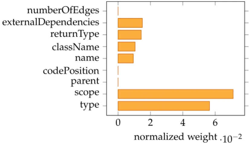
kernels are histogramkernels, which build a histogram over features of the structured datum xand use those as vectorial representationφ(x). Examples include histograms over the lengths of shortest paths in a graph(Borgwardt and Kriegel2005), histograms over subtree types and their position (Aiolli, Martino, and Sperduti2015), and histograms over hidden states of a Markov model trained on the structured datum (Bacciu, Errica, and Micheli2018).

Another approach to explicit kernelsrelies on learning the spatial mappingφ, for example via a neural network (Bacciu, Gallicchio, and Micheli2016; W.-b. Huang et al.

2015; Mehrkanoon and Suykens2018; Yanardag and Vishwanathan2015; Z. Yang et al.

2015). This relateskernelsto the field ofrepresentation learningfor structured data, which has received heightened attention in recent years (Bengio, Courville, and Vincent2013; LeCun, Bengio, and Hinton2015). For example, we can learn vectorial representations of sequential data via recurrent neural networks (Cho et al. 2014; Chung et al. 2015; Hochreiter and Schmidhuber1997; Jaeger and Haas2004; Sutskever, Vinyals, and Q. V. Le

2014), we can learn tree representations via recursive neural networks (Gallicchio and Micheli 2013; Irsoy and Cardie2014; Pollack1990; Socher, Perelygin, et al.2013; Sperduti and Starita 1997), and we can learn graphrepresentations via recurrent, recursive, or convolutional networks on graphs (Bacciu, Errica, and Micheli 2018; Gallicchio and Micheli 2010; Garcia Duran and Niepert2017; Hamilton, Ying, and Leskovec2017).

In terms of implicit kernels, a popular strategy involves representing a structured datum in terms of constituent parts and constructing an overallkernelas a sum over

kernelsbetween the constituents, such as path and walkkernels(Borgwardt and Kriegel

2005; Da San Martino and Sperduti 2010; Feragen et al. 2013) or Weisfeiler-Lehman

kernels(Shervashidze et al.2011). Once a structure kernel has been constructed, it is also possible to combine multiple kernels in linear combinations with non-negative weights, which has been dubbed multiple kernel learning (Aiolli and Donini 2015; Gönen and Alpaydın2011). Alternatively, one can perform an approach similar to metric learning by adjusting the parameters of a kernel to the data at hand, as has been done for biological sequence alignmentkernels(Saigo, Vert, and Akutsu2006).

Note that only fewkernelspermit intuitive interpretation. In particular, the subtree

kernels of Aiolli, Martino, and Sperduti (2015) could be interpreted in terms of the subtrees that are contained in both input trees, and the alignment kernel of Saigo, Vert, and Akutsu (2006) permits to pinpoint the elements that are different and equal in both inputsequences. However, the latter is only possible because the kernel is constructed based on anedit distance. Indeed,edit distanceshave the distinct advantage that they are not only interpretable, but actionable, in the sense that an edit distance tells us precisely what we need to change to reduce theedit distancebetween two structured data. Therefore, we focus onedit distancesin our work.

2.3 e d i t d i s ta n c e s

Anedit distancebetween two structured data ¯xand ¯yis defined as the effort needed to transform ¯x into ¯y. More precisely, anedit distanceis defined as the cost of the cheapest

edit scriptwhich transforms ¯xinto ¯y, and different notions ofedit scriptsyield different kinds ofedit distances. The first works onedit distancesare by Levenshtein (1965) as well as Damerau (1964) who independently devised a simple distance measure to count the number of spelling mistakes in a written sentence by defining it as the number of characters that have to be deleted, inserted, or changed to arrive at the correct version. Later, multiple researchers discovered dynamic programming algorithms to compute these notions of distance efficiently (Navarro2001). T. F. Smith and Waterman (1981) and Gotoh (1982) have later extended this basic work to computeedit distancesbetween RNA, DNA, and protein sequences in terms of their amino acid notation. Further, Tai (1979) and Zhang and Shasha (1989) have provided edit distance versions fortrees. Indeed, orderedtreesand ordered directed acyclic graphs are the most complex data structure for which we can compute theedit distanceefficiently as theedit distancefor unordered

treesand forgraphswith cycles are provably NP-hard (Zhang, Statman, and Shasha1992; Zeng et al.2009).

In this section, we describeedit distanceapproaches forsequences,trees, andgraphs, with a special focus onedit distancesonsequencesandtrees, because these are efficiently computable.

2.3.1 Sequence Edit Distance

We begin our description of sequence edit distancesby formally defining sequences,

editsoversequences,cost functions, and finallyedit distances. While these definitions capture the general intuition behind sequence edit distances, they are insufficient to

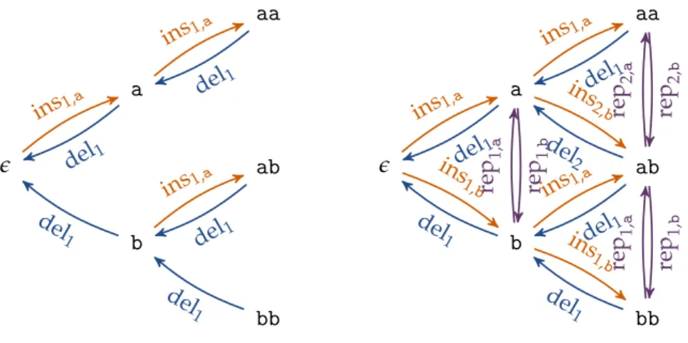
e a b aa ab bb ins1,a ins1,a ins1,a del1 del 1 del1 del1 del 1 e a b aa ab bb ins1,a ins 1,_b ins1,a ins 2,_b ins1,a ins 1,_b del1 del 1 del1 del 2 del1 del 1 rep 1, b rep 1, a rep 2, b rep 2, a rep 1, b rep 1, a

Figure 2.1:Left: A graphical representation of theedit set∆={del1, ins1,a}over thealphabet A = {a,b,c}. All possible sequences overA are nodes of the graph, and twosequences are connected if asequence editin∆exists that transforms the firstsequenceinto the second. Right: A similar graphical representation for theedit setover thesignatureSALI= ({del},{rep},{ins}).

derive efficient algorithms. Therefore, we introduce algebraic dynamic programming

(Giegerich, Meyer, and Steffen2004) as an alternative formalism to describesequence edit distances that is strong enough to yield results regarding metric properties and efficient computations. Note that we go into some detail regarding sequence edit distancesat this point because we later build upon our concepts and notations to learn these edit distancesin Chapter3.

Definition 2.5 (Alphabets, Sequences, Sequence Edits, Edit Sets, Edit Scripts). Let Abe some arbitrary set. We call such a set analphabet. We define asequenceover Aas a finite list of elements ¯x= x1. . .xmfromA. We callmthelengthof ¯x, denoted as|x¯|. We denote

theempty listase. We denote the set of all possiblesequencesoveralphabetAasA∗.

We define asequence editas a functionδ:A∗ → A∗. We call a set∆ofsequence edits

an edit set. We define anedit script over∆as asequenceover∆. We define the application

¯

δ(x¯) of anedit script δ¯ = δ₁. . .δT ∈ ∆∗ to a sequence x¯ as the function composition

δT◦. . .◦δ1(x¯), whereδ◦δ0(x¯):=δ(δ0(x¯)). If ¯δ =e, we define ¯δ(x¯):= x¯.

As an example, consider thealphabetA={a,b,c}. Then,e,a,abc, andaaaare all

sequencesoverA. Now, consider thesequence editdel1 :A∗ → A∗, which we define as del1(x1. . .xm):= x2. . .xm, and del1(e) =e. Applying del1to thesequenceabcresults in del1(abc) = bc. Accordingly, theedit scriptdel1del1 results in del1del1(abc) = c. Con-versely, consider thesequence editins1,a :A∗ → A∗, which we define as ins1,a(x¯) =ax¯. Applying ins1,a thesequenceabcresults in ins1,a(abc) =aabc. The set∆={del1, ins1,a} is anedit set.

We can interpret anedit setover some alphabetAin terms of agraphG = (V,E)by setting the nodes asV =A∗_{and constructing an edge(x¯, ¯y)∈Eif and only if there exists} asequence editδ∈ ∆such that δ(x¯) =y¯. This graphical view is particularly insightful in intelligent tutoring systems, where we can interpret the graphas the space of all possible states a student could visit on their way to a solution of a learning task. We therefore cover this interpretation in more detail in Chapter6(in particular, refer to Definition6.2).

Figure2.1(left) shows an excerpt of thisgraphfor our example above. Thesequence edit distanceis the shortest path distance in thisgraphif we set the length of all edges to the values of acost function, which we define as follows.

Definition 2.6(Cost Function, Sequence Edit Distance). LetAbe analphabetand let∆ be anedit setoverA. Then, we define acost functionover∆as a functionc:∆× A∗ _→R. We callc(δ, ¯x)the costof applyingδ to ¯x. Accordingly, we define the cost of applying an

edit scriptδ¯= δ1. . .δT to ¯x recursively asc(δ, ¯¯ x):=c(δ1, ¯x) +c(δ2. . .δT,δ1(x¯))with the base casec(e, ¯x) =0.

We define theedit distanced_∆,c according to∆andcas the following function.

d_∆,c :A∗× A∗ →R d_∆,c(x¯, ¯y):=min ¯ δ∈∆∗ n c(δ, ¯¯ x) δ¯(x¯) =y¯ o (2.12)

In other words: Theedit distancebetween ¯xand ¯yis the cost of the cheapestedit script

transforming ¯xto ¯y. Consider theedit set∆= {del1, ins1,a}above in combination with thecost function c(δ, ¯x) =1, independent of the input. Then, we obtain d_∆,c(e,a) =1,

d_∆,c(e,aa) =2, andd∆,c(bb,ab) =2.

While conceptually insightful, the definition ofedit distancesvia anedit setand acost functionhas severe practical limitations. First, anedit setneeds to be infinitely large if we wish to address arbitrarily longsequences, which poses a challenge in definition. Second, the concepts of an edit setand a cost function are too general to permit conclusions regarding metric properties. For example, ouredit distanceabove is not metric because it is not symmetric. However, we require certainty about self-equality and symmetry in order to ensure that aedit distanceispseudo-Euclidean. Third, the space of all possible

edit scripts over an infinite edit set is not efficiently searchable, preventing us from computing theedit distancein polynomial time.

As such, we sorely need an alternative formalism to express a subclass of edit distancesthat are efficiently computable, and this subclass needs to be expressive enough to include alledit distancesthat are interesting to us. As it turns out, the framework of

algebraic dynamic programmingis exactly what we need.

2.3.2 Algebraic Dynamic Programming

Algebraic dynamic programming (ADP)has been introduced by Giegerich, Meyer, and Steffen (2004) as adiscipline of dynamic programming over sequence data. In particular, the authors suggest to formalize potential solutions for a problem over sequential data as trees, generated by a regular tree grammar, and to find an optimal solution by essentially parsing the problem input via the grammar (Giegerich, Meyer, and Steffen2004). Note that this approach is highly general and encompasses diverse sequential problems far beyondedit distancecomputation, such as optimal RNA folding, hidden Markov model inference or scoring of phylogenetic trees (Siederdissen, Prohaska, and Stadler2015). In this section, we focus particularly onedit distancesand simplify the generalADPtheory for this purpose. Still, all our definitions follow strictly from the general case as described by Giegerich, Meyer, and Steffen (2004).

Note that we utilize theADPformulation as basis forsequence edit distancelearning later in Chapter 3. We also show metric properties and efficient computability there.

In this section, we focus on definitions. In particular, we introduce three ingredients which suffice to specify any typical sequence edit distance in the literature, namely

signatures, which capture the kinds ofeditsthat can be applied,algebrae, which capture how expensive these kinds ofeditsare, andedit tree grammars, which specify howedits

can be combined intoedit scripts. First, we begin withsignatures.

Definition 2.7 (Signature, Signature Edit Set). We define asignatureS as a triple of finite sets S = (Del, Rep, Ins), which are pairwise disjoint, that is Del∩Rep = Del∩Ins =

Rep∩Ins=∅. We callS non-trivialif neither Del nor Ins are empty.

LetA be an alphabet and S = (Del, Rep, Ins)be a signature. Then, we define for each element del∈Del and each natural numberi∈Nthe function deli :A∗ → A∗ as

deli(x1. . .xm):=x1. . .xi−1xi+1. . .xm ifi≤ m, and deli(x¯):= x¯ ifi>m.

For each element rep∈Rep, each elementy∈ A, and each natural numberi∈N, we define the function rep_i,y: A∗ _{→ A}∗ _{as rep}

i,y(x1. . .xm):= x1. . .xi−1yxi+1. . .xm ifi≤m,

and rep_i,y(x¯):=x¯ ifi> m.

Finally, for each element ins ∈ Ins, each elementy ∈ A, and each natural number i∈ N, we define the function insi,y :A∗ → A∗ as insi,y(x1. . .xm):= x1. . .xi−1yxi. . .xm

if i≤m+1, and insi,y(x¯):=x¯ ifi> m+1.

We define theedit set∆S,Awith respect to thesignatureS = (Del, Rep, Ins), and the alphabetAas follows.

∆S,A ={deli|del∈Del,i∈N}∪ (2.13)

{rep_i,y|rep∈Rep,i∈N,y ∈ A}∪ {insi,y|ins∈ Rep,i∈N,y∈ A}

As an example, consider one of the simplest non-trivialsignatures, ALI = ({del},

{rep},{ins}), which contains one kind of deletion, replacement, and insertion respectively and corresponds to the string edit distance of Levenshtein (1965). An excerpt of the graphical representation of the edit set ∆_ALI,{a,b,c} is shown in Figure2.1(right). Note that, as a user of the framework, we only need to specify a small signatureS, and the infinitely largeedit set∆S,A follows automatically. Also note that we can re-use the same signaturefor arbitraryalphabets, which simplifies specification.

Now that we have specified anedit set, we only need acost function to obtain an

edit distance. Following theADPframework, we generate acost functionbased on the

signaturevia the vehicle of analgebra.

Definition 2.8(Algebra, Algebra Cost Function). LetAbe analphabet, letS = (Del, Rep, Ins)be asignature, let(A →R)denote the set of functions mapping fromAto the real numbers R, and let(A × A →R)denote the set of functions mapping fromA × Ato the real numbersR.

Then, we define analgebraF overS andAas a triple of functionsFS,A= (FDel,FRep,

F_Ins), where F_Del : Del → (A → R),F_Rep : Rep → (A × A → R), and F_Ins : Ins → (A →_R).

As a shorthand, we denote the functionF_Del(del)ascdelfor all del∈Del, we denote

We define the cost functioncF with respect to analgebraF = (FDel,FRep,FIns)as the followingcost functionover ∆S,A.

cF(δ, ¯x):=            c_del(xi) if δ =deli,i≤ |x¯| crep(xi,y) if δ =rep_i,y,i≤ |x¯| cins(y) if δ =insi,y,i≤ |x¯|+1 0 otherwise (2.14)

As a notational shorthand, we denote theedit distanced_∆S,A,cF asdS,F.

As an example, consider the standard stringedit distanceof Levenshtein (1965), which corresponds to thesignatureS_ALI= ({del},{rep},{ins}), and thealgebraF_ALIwith the functions

cdel(x):=cins(x):=1 and crep(x,y):=

(

1 ifx6=y

0 ifx= y ∀x,y∈ A (2.15) An advantage in specifying acost function via analgebrais that we only need to specify the cost of edit types, which then automatically generalizes over the entire, infinitely largeedit set∆S,A.

An issue with the formalism ofedit scripts is that it is highly redundant, that is,edit scriptscan make detours before arriving at their final result. For example, the twoedit scriptsdel1 and ins1,arep_1,bdel2del1have exactly the same output for every possible input

sequence, but the latter makes detours, namely inserting the lettera, replacing it withb, and deleting it again, in addition to performing the actual action, namely deleting the first character in the inputsequence.

To express only those edit scriptsthat avoid such detours, we introduce thescript treeconcept.

Definition 2.9(Script Trees, Yield, Tree Cost). LetAbe analphabetwith $, match /∈ A, and let S = (Del, Rep, Ins) be a signature with $, match /∈ Del∪Rep∪Ins. Then, we define ascript treeδ˜overS andAas one of the following.

˜ δ =$,

˜

δ =match(x, ˜δ0,x) wherex∈ A, and ˜δ0 is ascript tree, ˜

δ =del(x, ˜δ0) where del∈ Del,x∈ A, and ˜δ0 is ascript tree, ˜

δ =rep(x, ˜δ0,y) where rep∈Rep,x,y∈ A, and ˜δ0 is ascript tree, or ˜

δ =ins(δ˜0,y) where ins∈Ins,y∈ A, and ˜δ0 is ascript tree. We define the set of all possiblescript treesoverS andAasT(S,A).

Let ˜δbe ascript treeoverS andA. Then, we define theyieldY(δ˜)∈ A∗× A∗of ˜δ as follows. Y(δ˜):=                (e,e) if δ˜=$ (xx¯,xy¯) if δ˜=match(x, ˜δ0,x) and(x¯, ¯y) =Y(δ˜0) (xx¯, ¯y) if δ˜=del(x, ˜δ0) and(x¯, ¯y) =Y(δ˜0) (xx¯,yy¯) if δ˜=rep(x, ˜δ0,y) and(x¯, ¯y) =Y(δ˜0) (x¯,yy¯) if δ˜=ins(δ˜0,y) and(x¯, ¯y) =Y(δ˜0)

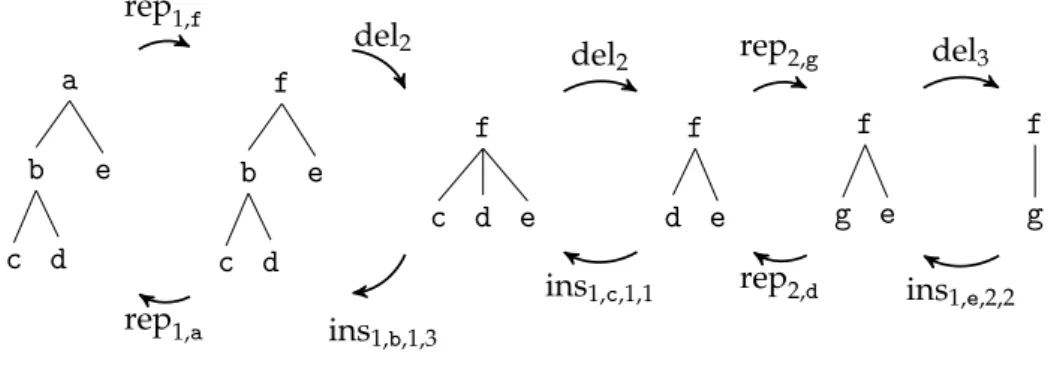
a ca cc c b

ins1,c rep2,c del₁ rep1,b

match a $ a ins c match a $ a ins c rep c $ a rep c $ a rep b $ a

Figure 2.2:An example for the translation of anedit scriptto ascript tree. The top row displays the sequence edits in theedit script which successively convert the sequence x¯ = a into the

sequencey¯=b. The bottom row shows thescript treecorresponding to the partialedit scriptup to the point of thesequenceat the top.

Further, we define thesize|δ˜| ∈N0 of ˜δ as follows.

|δ˜|:=

(

0 if ˜δ= $

1+|δ˜0| if∃δ˜0 : ˜δ∈ {match(x, ˜δ0,x), del(x, ˜δ0), rep(x, ˜δ0,y), ins(δ˜0,y)}

LetF be analgebraoverS andA. Then, we define thecost cF(δ˜)of ˜δ according toF as follows. cF(δ˜):=                0 if δ˜=$ cF(δ˜0) if δ˜=match(x, ˜δ0,x) c_del(x) +cF(δ˜0) if δ˜=del(x, ˜δ0) crep(x,y) +cF(δ˜0) if δ˜=rep(x, ˜δ0,y) cins(y) +cF(δ˜0) if δ˜=ins(δ˜0,y)

As an example, consider thescript treeδ˜=del(a, ins($,b))over thesignatureS_ALI = ({del},{rep},{ins})and thealphabetA={a,b}. Theyield of this tree is

Y(δ˜) = aY1 ins($,b) ,Y2 ins($,b) =aY1($),bY2($) = (a,b).

The size of the tree is |δ˜| = 1+|ins($,b)| = 2+|$| = 2. Finally, the cost of the tree according to algebraF_ALIfrom above is given as

cF(δ˜) =c_del(a) +cF ins($,b)

=c_del(a) +cins(b) +cF($) =cdel(a) +cins(b).

Intuitively, thescript treehas the purpose to jointly represent somesequencex¯, some

edit script δ, and the resulting¯ sequence δ¯(x¯). As mentioned above, however, the relation between edit scripts and script trees is not one-to-one, because script trees represent onlyedit scriptswhich avoid detours - at least extreme detours where we insert symbols that are not present in the targetsequence. Indeed, omitting such detours ensures that for any two sequences x¯ and ¯y the search space of possible script trees δ˜ with the

yieldY(δ˜) = (x¯, ¯y)is guaranteed to be finite, even though the set ofedit scripts which transform ¯x to ¯y may well be infinite. This drastic limitation in the search space also enables us to compute the resultingedit distancesefficiently (refer to Chapter3).

A final limitation of our framework until now is that we can not express additional contraints on theedit distance. Such constraints occur in extensions of the standardedit distance, such as the local alignmentdistanceof T. F. Smith and Waterman (1981), which permits cheaper deletions or insertions at the end of the input sequences, but not before, or the affine alignment distance of Gotoh (1982), which permits cheaper deletions or insertions if they occur in bulk. We can incorporate such constraints in form of anedit tree grammar.

Definition 2.10(Edit Tree Grammar, Tree Language, Grammar Edit Distance). Let S = (Del, Rep, Ins)be asignature with $, match /∈ Del∪Rep∪Ins. Then, we define anedit

tree grammar G as a quartupleG = (Φ,S,R, S), where Φis a finite set, which we call

nonterminal symbols, such that Φ∩(Del∪Rep∪Ins∪ {match, $}) =∅, S∈Φ, andR is

a finite set of so-calledproduction rulesof the form A::= δBor the form A::= $, where A,B∈ Φandδ ∈Del∪Rep∪Ins∪ {match}.

Per convention, we denote multiple production rules A ::= δ1B1, . . ., A ::= δTBT,

A::=$ with the same left-hand side Aas A::= δ1B1|. . .|δTBT|$.

LetAbe analphabet, let A,B∈ Φ,x,y∈ A, del∈Del, rep∈Rep, and ins∈Ins. We say that $ can bederived in one stepfrom Avia G, denoted asA→1

G $, if theproduction rule A::= $ is inR. Similarly, we say that A→1

G match(x,B,x)if A::= matchB∈ R, we say that A →1

G del(x,B) if A ::= delB ∈ R, we say that A →1G rep(x,B,y) if A::=rep(x,B,y)∈ R, and we say that A→1

G ins(B,y)if A::=insB∈ R.

We say that an expression ˜δ can be derived in T+1 steps from A ∈ Φ for T ∈ N, denoted as A→T+1

G δ˜if one of the following cases holds. ˜

δ =match(x, ˜δ0,x) for some expression ˜δ0, and there exists a B ∈ Φ such that A →1_G match(x,B,x), as well asB→T

G δ˜0. ˜

δ =del(x, ˜δ0) for some expression ˜δ0, and there exists aB∈Φsuch that A→1_G del(x,B), as well asB→T

G δ˜0. ˜

δ =rep(x, ˜δ0,y) for some expression ˜δ0, and there exists a B ∈ Φ such that A →1_G rep(x,B,y), as well asB→T

G δ˜0. ˜

δ =ins(δ˜0,y) for some expression ˜δ0, and there exists aB∈ Φsuch that A→1_G ins(B,y), as well asB→T

G δ˜0.

We say that ˜δcan bederived in arbitrarily many steps fromA, denoted as A→∗_G δ, if˜ there exists anyT∈Nsuch that A→T

G δ. We define the˜ tree languageofG with respect toAas follows.

L(G,A):={δ˜∈ T(S,A)|S→∗_G δ˜}

LetF be analgebraoverS andA, and let ¯x, ¯y∈ A∗. Then, we define theedit distance

between ¯xand ¯ywith respect toG andF as follows. dG,F(x¯, ¯y):= min

˜

δ∈L(G,A)

Note that includingedit tree grammarsinto the formalism does not restrict expressiv-ity. For everysignatureS = (Del, Rep, Ins)and everyalphabetAwe can recover the set

T(A,S)as thetree languageof the trivialedit tree grammar

GS = ({S},S,{S ::=$} ∪ {S ::= δS|δ ∈Del∪Rep∪Ins∪ {match}}, S).

As an example, consider thesignatureS_ALI= ({del},{rep},{ins})and the following

edit tree grammar G_ALI.

GALI = ({A},SALI,R, A) where R={A ::=matchA|delA|repA|insA|$} (2.16) For thisedit tree grammarand anyalphabetAit holds:L(G_ALI,A) =T(A,S_ALI).

Now, consider the twosequences x¯ =aand ¯y=bover thealphabetA={a,b}and consider thealgebraF_ALIfrom Equation2.16. To compute theedit distancebetween ¯x and ¯y with respect toG_ALI andF_ALI, we need to consider all script treesδ˜that can be generated via G_ALIand have theyieldY(δ˜) = (x¯, ¯y) = (a,b). These are only thescript treesdel(a, ins($,b)), rep(a, $,b), and ins(del(a, $),b), which can be derived from A as follows.

A→1_G del(a, A)→1_G del(a, ins(A,b))→1_G del(a, ins($,b)),

A→1_G rep(a, A,b)→1_G rep(a, $,b), and A→1_G ins(A,b)→1_G ins(del(a, A),b)→1_G ins(del(a, $),b)

The cheapest of thesescript treesis rep(a, $,b)with a cost of 1, whereas both otherscript treeshave a cost of 2. Therefore, we obtaindG,F(a,b) =1. Note that this is equal to the edit distancedS,F(a,b). This is no coincidence. Indeed, we show in Chapter3that any edit distancedS,F is equivalent to theedit distanceover its trivialedit tree grammardGS,F if the algebraF ensures thatedit scriptswhich make detours can never be cheaper than

edit scriptswhich do not. We also show that any suchedit distance adheres to metric axioms if thealgebradoes as well.

Now, let us return to our original motivation for edit tree grammars, namely to incorporate additional constraints. As an example, consider the local alignment distance of T. F. Smith and Waterman (1981), where the suffices of bothsequences are considered irrelevant if the edit distance between them exceeds a constant. We can model this behavior by introducing new symbols in our signature called skipl, skipl,o, skipr, and skipr,o as follows.

S_LOCAL:= ({del, skipl, skipl,o},{rep},{ins, skipr, skipr,o}) (2.17) We extend theedit tree grammarG_ALIas follows.

G_LOCAL:=({A, S},S_LOCAL,R, A), where

R ={A ::=matchA|repA|delA|insA|$}∪ {A ::=skipl,oS|skipr,oS}∪

{S ::=skiplS|skiprS|$}

To ensure a constant cost for ignoring the suffices of both inputsequences, thealgebra

dGALI,F(aaacac,ccbbb) =6 rep c rep c rep b rep b rep b del $ c a c a a a dGLOCAL,F(aaacac,ccbbb) =6 del del del match c del match c skipr,o b skipr b skipr b $ c a c a a a dGAFFINE,F(aaacac,ccbbb) =5 skipl,o skipl skipl match c del match c skipr,o b skipr b skipr b $ c a c a a a

Figure 2.3:The cheapestscript treesδ˜withyieldY(δ˜) = (aaaacac,ccbbb)according to theedit tree grammarsGALI(left),GLOCAL(middle), andGAFFINE(right), respectively. In all cases, we use

thealgebraFAFFINEin Equation2.19.

If it is possible to use skipl and skiprnot only in the end but at any point during the edit process, we obtain a scheme, which follows the affine gap cost logic of Gotoh (1982).

G_AFFINE:=({A, S},S_LOCAL,R, A), where (2.18)

R={A ::=matchA|repA|delA|insA|$}∪ {A ::=skipl,oS|skipr,oS}∪

{S ::=skiplS|skiprS|matchA|repA|$}

A comparison of G_ALI, G_LOCAl, and G_AFFINE is shown in Figure 2.3 for the example

sequencesx¯ =aaacacand ¯y=ccbbb, using the followingalgebraF_AFFINE.

cdel(x):=c_skipl,o (x):=cins(x):=cr_skip,o (x):=1 ∀x∈ A (2.19) cl_skip(x):=cr_skip(x) =0.5 ∀x∈ A

crep(x,y):=crep(y,x):=

(

1 ifx 6=y

0 ifx =y ∀x,y∈ A

we build upon this ADPrepresentation and show that the edit distances defined via

ADPare indeed pseudo-metrics, and that they are efficiently computable.

Now, that we have coverededit distancesoversequences, we can turn towards more complicated data structures, namelytrees.

2.3.3 Tree Edit Distance

The firstedit distance ontrees has been suggested by Tai (1979) as a straightforward extension of the standard stringedit distance of Levenshtein (1965). In particular, Tai (1979) used the same edit set as the standard string edit distance, namely deletions, insertions, and replacements, and defined the overall edit distancebetween twotrees

˜

x and ˜y as the cost of the cheapestedit scriptδ, which transforms ˜¯ x to ˜y. To compute the tree edit distancebetween twotreesof sizem, Tai (1979) proposed aO(m6)dynamic programming algorithm, which was later improved by Zhang and Shasha (1989) toO(m4_), and by Demaine et al. (2009), Pawlik and Augsten (2011), and Pawlik and Augsten (2016) to O(m3), which is provably optimal for thisedit set(Demaine et al. 2009).

By constraining theedit set, we can further improve the worst-case bound (Bille2005). For example, the tree edit distanceof Selkow (1977) permits only deletions or insertions of entire subtrees, which reduces the computational complexity to O(m2).

In this section, we focus on the classictree edit distanceof Zhang and Shasha (1989) for multiple reasons. First, it provides a proper generalization over the standard string

edit distance, and indeed the algorithm of Zhang and Shasha (1989) gracefully degrades to the algorithm of Levenshtein (1965) for the special case of sequential input. Second, it can be seen as the upper limit of structural complexity that can be handled by polynomial-time algorithms, given that both the extensions to graphs, as well as the extension to unordered treesare provably NP-hard (Zhang, Statman, and Shasha 1992; Zeng et al.

2009). Finally, theedits, namely single-node replacements, deletions, and insertions, are simple enough to be intuitive and actionable to humans, e.g. students in intelligent tutoring systems (Rivers and Koedinger2015; Paaßen, Hammer, et al. 2018). We describe the tree edit distancein detail here because we build upon the notation and concepts introduced in this chapter to learntree edit distanceparameters in Chapter4.

We first introducetreesandforestsas central objects of study for this section, then go on to introduce tree editsand cost functionsfor suchtree edits, and finally define auxiliary concepts ontrees, which will enable us to derive thetree edit distancealgorithm of Zhang and Shasha (1989).

Definition 2.11(Tree, Forest, Pre-Order). LetAbe analphabet. We define atreex˜ over

Arecursively as ˜x =x(x˜1, . . . , ˜xR), wherex∈ Aand ˜x1, . . . , ˜xR is a (possibly empty) list

of treesoverA. We denote the set of alltreesover AasT(A).

We callxthe label of ˜x, also denoted asν(x˜), and we call ˜x1, . . . , ˜xR the children of ˜x,

also denoted as ¯$(x˜). If atreehas no children (i.e. R =0), we call it aleaf. In terms of notation, we will generally omit the brackets for leaves, i.e. xis a notational shorthand for x().

We call a list oftreesX = x˜1, . . . , ˜xR fromT(A)aforestoverA, and we denote the

set of all possibleforestsover AasT(A)∗_{. We denote the emptyforestas e.}

We define thesize |X| of a forestX = x˜1, . . . , ˜xR recursively as |X| = 1+|$¯(x˜1)|+

We define thepre-orderπ(X)of aforest X=x˜1, . . . , ˜xR recursively as the listπ(x˜):= ˜

x1,π($¯(x˜1)),π(x˜2, . . . , ˜xR)if X6=eand asπ(X) =eif X=e. We denote theithtreein the pre-order ofXas ˜xi, and the labelν(x˜i)of ˜xi as xi.

Regarding this definition, note that any tree is a special case of a forest, that the children of atreealso form aforest, and that any single element fromAis a trivial case of atree.

As an example, consider thealphabetA= {a,b}. Some treesoverAarea,b,a(a), a(b),b(a,b), anda(b(a,b),b). An exampleforestover this alphabet is(a,b,b(a,b)). Now, consider the exampletree x˜ = a(b(c,d),e)The label of ˜x isν(x˜) =a, and the children are ¯$(x˜) =b(c,d)ande. The size of ˜xis

|x˜|=1+|b(c,d),e|+|e|

=1+ (1+|c,d|+|e|) +0

=2+ (1+|e|+|d|) + (1+|e|+|e|)

=3+ (1+|e|+|e|) +1

=3+1+1=5.

Intuitively, the pre-order of ˜xis the list of all subtrees of ˜xaccording to depth-first search. Strictly using the definition, we obtain:

π(x˜) =x˜,π(b(c,d),e),π(e)

=x˜,b(c,d),π(c,d),π(e),π(e)

=x˜,b(c,d),c,π(e),π(d),e,π(e),π(e),

=x˜,b(c,d),c,d,π(e),π(e),e,

=x˜,b(c,d),c,d,e.

Next, we define how to manipulate trees via tree edits. Note that tree edits are analogous tosequence editsin Definition2.5.

Definition 2.12(Tree Edits). We define atree editδas a functionδ :T(A)∗ → T(A)∗. We call a set∆oftree editsanedit set. We define anedit scriptover∆as asequenceover∆. We denote the set of all possibleedit scriptsoveredit setas∆∗. We define the application

¯