10
© Global Society of Scientific Research and Researchers http://asrjetsjournal.org/
On the Efficiency of Outlier Generating Mechanisms in
Multivariate Time Series
Olusesan Oluyomi Olufolabo
a*, Olanrewaju Ismail Shittu
b, Kazeem Adesola
Adepoju
ca
Department of Statistics, Yaba College of Technology, Lagos, Nigeria
b,c
Department of Statistics, University of Ibadan, Ibadan, Nigeria
a Email:[email protected] b Email: [email protected] c Email: [email protected] Abstract
In this paper, two new outlier generating mechanisms for the detection of outliers in multivariate time series setting were derived. This is achieved by specifying two-variable vector autoregressive models and assuming additive and convolution effect of outliers on time series data. The magnitude and variance of outlier were derived for the generating models by method of least squares. Also a modified test statistics were developed to detect single outliers both in the response and explanatory variables. In order to establish the validity and efficiency of the derived models, the models were applied to both simulated and existing data. The results from the analysed data were also compared to some existing models and the result showed that the convolution model is best in terms of the number of outliers detected and the residual variance. This result confirms the finding in previous studies of outlier detection in univariate time series.
Keywords: Additive outlier; Convolution outlier; Innovative outlier; Multiplicative outlier; Vector auto regressive.
1. Introduction
The problem of outlier detection in time series has gained much attention in recent times and various methods of detection are available, but in most cases, it is limited to univariate time series.
--- * Corresponding author.
11
It is a known fact, that in time series analysis, outliers can cause biases in parameter estimation as well as inappropriate predictions, resulting in misleading conclusion [28]. The essence of outlier detection is to discover the unusual data; whose behaviour is very exceptional when compared to the rest of the data set. Examining the extraordinary behaviour of outliers
will surely help to uncover the valuable knowledge hidden behind them and to help the decision makers to improve on the quality of data.
Generally, detection methods are divided into two parts: univariate and multivariate methods. In univariate methods, observations are examined individually while in multivariate methods, associations between variables in the same dataset are taken into account.
Several outlier detection methods have been proposed for univariate time series including [11,8,9,26,1,14 and 32]. All the listed works were based on time domain and almost all make use of iterative procedure in the outlier detection process. However, [25] in their work considered the identification of outliers in frequency domain using the spectral method.
On the detection of outlier in multivariate time series, [12] made use of projection pursuit technique while [3] proposed the Independent Component Analysis (ICA) as a tool capable of identifying the locations of multiple outliers in multivariate time series. The authors [10] used meta-heuristic methods to detect additive outliers in multivariate time series. The work of [13] introduced the coefficient of vector autocorrelation, obtained its influence function together with its distribution and used it to test the hypothesis of presence of outliers. [31] in his paper used an efficient two-phase algorithm for detecting outlying samples in multivariate time series datasets. The Bounded Coordinate System metric was used to measure the similarity between two multivariate time series samples, and the outlierness of a sample is measured by average distance to its k nearest neighbours. Then a heuristic and two pruning rules were utilized to quickly remove multivariate time series samples that are not possible outlier candidates, reducing significantly the distance computation among objects.
As a result of outlier masking effect of both Additive and Innovative on the estimates of parameters and the multiplicative effect on parameters estimated, [26] introduced two other types of outliers which are Convolution Outlier (CO) and Multiplicative Outlier (MO) for univariate time series. The work of [26] was extended to multivariate time series by [19] whereby two generating mechanisms; Innovative and Multiplicative were considered. It was concluded that Multiplicative outlier model was more sensitive to outlier with minimum standard error of the estimate.
For this paper, two outliers generating mechanisms; Convolution and Additive will be extended to multivariate time series and their performances in terms of outlier detection will be compared to the existing ones.
2. Methodology
In this section, by assuming that outliers have either Additive or Convolution effect on a series for bivariate time series and specifying two-variable Vector Autoregressive (VAR) models, the estimate of the parameter for the
12
two models will be derived and their corresponding test statistics developed.
2.1 Derivation of Outlier Generating Mechanisms for Additive Outlier (AO) Model
In this subsection outlier generating mechanism for additive outlier model will be derived.
Generally, an additive outlier represents an unexpected change in the value of one of the observations. It can appear as a result of a recording or measurement error or other single effect.
The additive outlier is defined as
) (T t t t
Z
X
=
+
ω
ξ
(1)where
X
t= (𝑥𝑥1𝑡𝑡,𝑥𝑥2𝑡𝑡,… … … . . 𝑥𝑥𝑘𝑘𝑡𝑡) is a k-dimensional time series, Zt is an outlier free time series that isassumed to follow the Autoregressive Moving Average of Order (p,q) i.e. ARMA (p,q),
) (T t
ξ
is a time indictor such thatξ
t(T)=
1
for all0
) (
=
=
T tand
T
t
ξ
otherwise, and 𝜔𝜔 = �ω
1, … ,ω
k�′ is the size or the magnitude of outlier.Now, given vector models
X
1tandX
2t such thatX
1tcontains outlier andX
2tis outlier free, the magnitude of such outlier and its corresponding variance can be obtained by specifying the two variable VAR(2) as:1 11 1 1 12 2 1 1 2 21 2 1 22 1 1 2 (2) t t t t t t t t X X X a X X X a ϕ ϕ ϕ ϕ − − − − = + + = + + (3)
where,
X
1tandX
1 1t− are the current and lag values of the response variable respectively,X
2tandX
2t−1 are current and lag values of the explanatory variable respectively.Now considering equation (3)
𝑋𝑋2𝑡𝑡= ∅21𝑋𝑋2𝑡𝑡−1+ ∅22𝑋𝑋1𝑡𝑡−1+ 𝑎𝑎1𝑡𝑡
When 𝑋𝑋2𝑡𝑡−1 is contaminated and assumed additive model, we have
𝑋𝑋2𝑡𝑡= ∅21�𝑍𝑍𝑡𝑡−1+ 𝜔𝜔𝜉𝜉𝑡𝑡−1(𝑇𝑇)� + ∅22𝑋𝑋1𝑡𝑡−1+ 𝑎𝑎1𝑡𝑡 (4)
13
𝑋𝑋2𝑡𝑡= ∅22 𝑋𝑋1𝑡𝑡−1+ 𝜙𝜙21 𝑍𝑍𝑡𝑡−1+ 𝜙𝜙21 𝜔𝜔𝜉𝜉𝑡𝑡−1(𝑇𝑇)
𝑋𝑋2𝑡𝑡= ∅22 𝑋𝑋1𝑡𝑡−1+ 𝜙𝜙21 𝜑𝜑(𝛽𝛽)𝜉𝜉𝑡𝑡−1+ 𝜙𝜙21 𝜔𝜔𝜉𝜉𝑡𝑡−1
𝑋𝑋2𝑡𝑡= ∅22 𝑋𝑋1𝑡𝑡−1+ 𝜙𝜙21 𝜉𝜉𝑡𝑡−1�𝜔𝜔 + 𝜑𝜑(𝛽𝛽)� Therefore, the general the additive model is given as
𝐴𝐴𝐴𝐴𝐴𝐴𝐴𝐴𝐴𝐴𝐴𝐴𝐴𝐴𝐴𝐴𝐴𝐴𝐴𝐴𝐴𝐴𝐴𝐴𝐴𝐴: 𝑋𝑋𝐴𝐴𝐴𝐴𝑡𝑡= 𝜙𝜙𝐴𝐴𝐴𝐴𝑋𝑋𝑗𝑗𝑡𝑡−1+ ∅𝐴𝐴𝑗𝑗𝜖𝜖𝑡𝑡−1 �𝜔𝜔 + 𝜑𝜑(𝛽𝛽)� (5)
2.1.1 Derivation of the Magnitude of Outlier for AO
With
X
1t=
ϕ
11X
1 1t−+
ϕ
12X
2 1t−+
a
1tas defined in equation (2)
Then,(
)
( )
( )
( )
( )
( )
( ) ( ) 11 12 2 1 1 ( ) ( ) 11 12 1(6)
T T t t t t t t T T t t t t t
Z
Z
X
a
a
a
ωξ
ϕ
ωξ
ϕ
θ β
ωξ
ϕ
θ β
ωξ
ϕ φ β
ϕ β
ϕ β
−+
=
+
+
+
+
=
+
+
+
l
( )
( )
( )
( )
12( )
( ) ) ( 111
tT t tT ta
ω
φ
ϕ
β
ωξ
β
φ
β
θ
φ
β
φ
β
θ
−
+
∈
+
=
−
( )
( )
( )
( )
( )
1
) ( 12 ) ( 11−
−
+
+
=
β
θ
β
φ
ωξ
β
ϕ
φ
ωξ
β
θ
β
φ
φ
T t t T t ta
(7)Summing the square of equation (1.9) over n we have
( )
( )
( )
( )
( )
∑
∑
= =
−
−
+
+
=
n t n t T t t T t ta
1 1 ) ( 12 ) ( 11 21
β
θ
β
φ
ωξ
β
ϕ
φ
ωξ
β
θ
β
φ
φ
(8)Differentiating equation (1.7) with respect to
ω
and setting to zero, we obtain the magnitude of outlier in the model as14
( )
( )
( )
( )
( )
0
1
2
ˆ
) ( 12 ) ( 1 11 2 2=
−
+
+
−
=
∂
∂
∑
= T t t T t n t A ta
ωξ
φ
ϕ
β
ωξ
β
θ
β
φ
φ
β
θ
β
φ
ω
l
(9)( )
( )
∑
( )
∑
∑
= = ==
−
+
+
n t n t t n t 1 1 12 1 11θ
β
ω
φ
ϕ
β
ω
0
β
φ
φ
( )
( )
( )
(
)
( )
( )
( )
t t
β
ϕ
φ
β
φ
β
θ
φ
φ
ω
ω
β
ϕ
φ
ω
φ
β
θ
β
φ
φ
12 11 11 12 11 111
0
+
=
−
=
−
+
+
( )
( )
( )
11 12 111
ˆ
φ
β
ϕ
φ
β
φ
β
θ
φ
ω
−
+
=
t A
( )(
)
11 121
1
ˆ
φ
φ
β
ϕ
ω
−
+
=
t A
(10)Therefore, the estimate of the variance is
( )
(
)
2 2 2 12 2 11ˆ
1
a AV
φ β ϕ σ
ω
ϕ
=
−
2 2 2 12 111
aϕ
φ β σ
ϕ
=
−
(11)With the estimates of mean and variance of the magnitude of AO derived, the test statistic for testing the presence of outlier for additive model is constructed as follows:
(
)
12 11 11 12 12 121
1
.
1
1
(12)
t i a t i aϕ
ϕ
λ
ϕ
ϕ σ
ϕ
λ
ϕ σ
+
−
=
−
+
=
l
l
15
2.2 Derivation of Outlier Generating Mechanisms for Convolution Outlier (MO) Model
The outlier effect on a given series may be either additive or innovative and the effect may be a combination of the two [26].
By this, we propose the convolution of the additive and innovative outliers for the multivariate setting as follows:
The innovative and additive models are defined respectively as follows:
( )
model
additive
for
model
innovative
for
) (T t t tA T t t tI
Z
X
Z
X
ωξ
ωξ
β
ϕ
+
=
+
=
The convolution involved adding both innovative and additive models [26]. This gives
( )
(
ϕ
β
)
ωξ
+
+
=
2
t tT1
tCZ
X
(13)For the general case of CO, now considering,
𝑋𝑋2𝑡𝑡= ∅21𝑋𝑋2𝑡𝑡−1+ ∅22𝑋𝑋1𝑡𝑡−1+ 𝑎𝑎1𝑡𝑡 as defined in equation (2) Assuming 𝑋𝑋2𝑡𝑡−1 is contaminated, we have
𝑋𝑋2𝑡𝑡= ∅21�2𝑍𝑍𝑡𝑡−1+ 𝜔𝜔𝜉𝜉𝑡𝑡(𝑇𝑇)(1 +𝜑𝜑(𝛽𝛽))� + ∅22𝑋𝑋1𝑡𝑡−1+ 𝑎𝑎1𝑡𝑡 (14) 𝑋𝑋2𝑡𝑡= 2∅21𝑍𝑍𝑡𝑡−1+ ∅21𝜔𝜔𝜉𝜉𝑡𝑡(𝑇𝑇)(1 +𝜑𝜑(𝛽𝛽)) + ∅22𝑋𝑋1𝑡𝑡−1+ 𝑎𝑎1𝑡𝑡 where 𝑍𝑍𝑡𝑡= 𝜑𝜑(𝛽𝛽)𝜉𝜉𝑡𝑡(𝑇𝑇)and 𝑍𝑍𝑡𝑡−1= 𝜑𝜑(𝛽𝛽)𝜉𝜉𝑡𝑡(𝑇𝑇) we then have 𝑋𝑋2𝑡𝑡= 2∅21𝜑𝜑(𝛽𝛽)𝜉𝜉𝑡𝑡(𝑇𝑇)+ ∅21𝜔𝜔𝜉𝜉𝑡𝑡(𝑇𝑇)(1 +𝜑𝜑(𝛽𝛽)) + ∅22𝑋𝑋1𝑡𝑡−1+ 𝑎𝑎1𝑡𝑡 (15) 𝑋𝑋2𝑡𝑡= 2∅21𝜑𝜑(𝛽𝛽)𝜉𝜉𝑡𝑡(𝑇𝑇)+ ∅21𝜔𝜔𝜉𝜉𝑡𝑡−1+ ∅21𝜔𝜔𝜉𝜉𝑡𝑡(𝑇𝑇)𝜑𝜑(𝛽𝛽) + ∅22𝑋𝑋1𝑡𝑡−1+ 𝑎𝑎1𝑡𝑡 𝑋𝑋2𝑡𝑡= ∅22𝑋𝑋1 𝑡𝑡−1+ 2∅21𝜑𝜑(𝛽𝛽)𝜉𝜉𝑡𝑡(𝑇𝑇)+ ∅21𝜔𝜔𝜉𝜉𝑡𝑡(𝑇𝑇)+ ∅21𝜔𝜔𝜉𝜉𝑡𝑡(𝑇𝑇)𝜑𝜑(𝛽𝛽) 𝑋𝑋2𝑡𝑡= ∅22𝑋𝑋1 𝑡𝑡−1+ 2∅21𝜑𝜑(𝛽𝛽)𝜉𝜉𝑡𝑡(𝑇𝑇)+ ∅21𝜔𝜔𝜉𝜉𝑡𝑡(𝑇𝑇)�1 + 𝜑𝜑(𝛽𝛽)� 𝑋𝑋2𝑡𝑡= ∅22𝑋𝑋1 𝑡𝑡−1+ ∅21𝜉𝜉𝑡𝑡(𝑇𝑇)[2𝜑𝜑(𝛽𝛽) + 𝜔𝜔(1 + 𝛽𝛽)] (16)
16 Therefore, in general, the CO generating mechanism is
𝐶𝐶𝐴𝐴𝐶𝐶𝐴𝐴𝐴𝐴𝐴𝐴𝐶𝐶𝐴𝐴𝐴𝐴𝐴𝐴𝐶𝐶𝐴𝐴𝐴𝐴𝐴𝐴𝐴𝐴𝐴𝐴: 𝑋𝑋𝐶𝐶𝐴𝐴𝑡𝑡= 𝜙𝜙𝐴𝐴𝐴𝐴𝑋𝑋𝑗𝑗𝑡𝑡−1+ ∅𝐴𝐴𝑗𝑗𝜉𝜉𝑡𝑡−1𝑇𝑇 [2𝜑𝜑(𝛽𝛽) + 𝜔𝜔(1 + 𝛽𝛽)] (17)
2.1.2 Derivation of Magnitude of Outlier for CO
Now, specifying
X
1t=
φ
11X
1t−1+
φ
12X
2t−1+
a
1t(18)
and substituting
X
tC in equation (18) gives( )
(
)
(
(
( )
)
)
t t T t t T t tZ
X
a
Z
( )1
112
1 ( )1
12 2 1 12
+
ωξ
+
ϕ
β
=
φ
−+
ωξ
+
ϕ
β
+
φ
−+
(19)( )
(
( )
)
[
( )
(
( )
)
]
( )
t t T t t T t ta
a
a
( )1
112
11
12 1 12
ϕ
β
+
ωξ
+
ϕ
β
=
φ
ϕ
β
−+
ωξ
+
ϕ
β
+
φ
ϕ
β
−+
( )
β
φ
ϕ
( )
β
φ
ϕ
( )
β
ωξ
(
ϕ
( )
β
)
φ
ωξ
(
ϕ
( )
β
)
ϕ
−
2
−−
= −−
1
+
+
1
+
2
a
t 11a
t 1a
1t 12
t 1 t(T) 11 t(T)( )
( )
[
2
ϕ
β
−
2
ϕ
β
φ
11−
1
]
=
φ
12ϕ
( )
β
t−1−
ωξ
t(T)(
1
+
ϕ
( )
β
)
+
φ
11ωξ
t(T)(
1
+
ϕ
( )
β
)
ta
(20)Summing and squaring equation (20) gives
( )
(
( )
)
(
( )
)
[
]
( )
( )
[
]
∑
∑
= = −−
−
−
+
+
−
=
n t n t T t T t t ta
1 2 11 1 2 11 1 12 21
2
2
1
1
φ
β
ϕ
β
ϕ
β
ϕ
ωξ
φ
β
ϕ
ωξ
β
ϕ
φ
(21)Differentiating equation (21) with respect to
ω
and equating to 0 we have( )
(
)
(
( )
)
( )
( )
[
2
2
1
]
0
1
1
2
2 11 11 2=
−
−
+
+
+
=
∂
∑
∂
φ
β
ϕ
β
ϕ
β
ϕ
φ
β
ϕ
ω
ta
` (22)( )
(
( )
)
(
( )
)
[
1
1
]
0
1 11 1 12−
+
+
+
=
∑
= − n t tω
ϕ
β
φ
ω
ϕ
β
β
ϕ
φ
( )
1(
1
( )
)
11(
1
( )
)
0
12ϕ
β
−−
ω
+
ϕ
β
+
φ
ω
+
ϕ
β
=
φ
t( )
(
1
+
ϕ
β
)
−
φ
11ωω
(
1
+
ϕ
( )
β
)
=
φ
12ϕ
( )
β
t−1ω
17
( )
(
)
(
( )
)
[
1
+
ϕ
β
−
φ
111
+
ϕ
β
]
=
φ
12ϕ
( )
β
t−1ω
( )
(
φ
)
(
ϕ
( )
β
)
β
ϕ
φ
ω
−
−
=
−1
1
ˆ
11 1 12 t C
(23)The corresponding variance is
( )
(
)
(
( )
)
2 2 12 2 2 11ˆ
V(
)
1
1
a Cϕ φ β σ
ω
ϕ
φ β
=
−
−
(24)Therefore, the test statistic is
( )
C C ie
S
ω
ω
λ
ˆ
.
ˆ
=
( )
(
)
(
( )
)
(
)
2(
( )
)
2 11 2 2 2 12 11 1 111
1
1
1
/
β
ϕ
φ
σ
β
ϕ
φ
β
ϕ
φ
β
ϕ
φ
λ
+
−
+
−
=
− a t i
(25)( )
(
)
(
( )
)
(
)
(
( )
( )
a)
tσ
β
ϕ
φ
β
ϕ
φ
β
ϕ
φ
β
ϕ
φ
12 11 11 1 121
1
*
1
1
+
−
+
−
=
− a t iσ
λ
1−
=
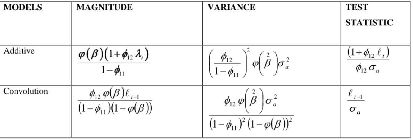
(26)Table 1: Summary of Estimates and Test Statistic for the two models when
X
1tcontains outlierMODELS MAGNITUDE VARIANCE TEST
STATISTIC Additive
( )
(
)
12 111
1
tϕ β
φ λ
φ
+
−
2 2 2 11 121
φ
ϕ
β
σ
aφ
−
(
)
a tσ
φ
φ
12 121
+
Convolution( )
(
φ
)
(
ϕ
( )
β
)
β
ϕ
φ
−
−
−1
1
11 1 12
t(
)
2(
( )
)
2 11 2 2 121
1
φ
ϕ
β
σ
β
ϕ
φ
−
−
a a tσ
1 −
18
3. Application
In this section, analysis of both simulated and real data sets will be used to test the validity and efficiency of the derived outliers generating mechanisms. In other to compare the performance of the two newly derived models with the existing ones, Data on Nigerian Bank Deposits and Loans from Annual Statistical Bulletin of the Central Bank of Nigeria, 2011 were made used of.
From the derived outlier generating mechanisms in section 2 and with the estimation of the magnitudes of outliers and their variances, the test statistics constructed will be used to detect the existence of outliers in both the generated series and real data.
For the simulated data, a uniform distribution is assumed with contaminated observation with varying sizes of 10, 50, and 100. The data were analysed with the R-package of version 3.0.1.
3.1 Analysis of Simulated Data when X1t Contains an Outlier
The results of the models on simulated data assuming a uniform distribution in terms of their outlier detection performance are tabulated below.
The sample sizes considered are 10, 50 and 100.
Table2: Summary of Result on Detection Rate of the Models on Simulated Data when
X
1t contains outlierN=10 N=50 N=100 Model Type No of outliers injected No of outliers detected % of outliers detected No of outliers injected No of outliers detected % of outliers detected No of outliers injected No of outliers detected % of outliers detected Additive 2 1 50 5 4 80 8 6 75 Convolution 2 2 100 5 5 100 8 8 100 Innovative* 2 0 0 5 2 40 8 2 25 Multiplicative* 2 2 100 5 4 80 8 5 80 Source* [19]
The Convolution model from the summary in Table2 had 100% outlier detection compared to Additive model as the sample size increases.
When compared with existing models, the Convolution model is most sensitive to outlying observations.
19
In order to investigate the performance of the proposed models, a pair of data on Deposit and Loan was used. The data was extracted from the Annual Statistical Bulletin of the Central Bank of Nigeria, 2011.
3.2.1. Assumed Model of Deposits and Loans
Here two cases are considered. The first case is when loan is contaminated.
The vector autoregressive model is given as
𝑋𝑋1𝑡𝑡= ∅11𝑋𝑋1𝑡𝑡−1+ ∅12𝑋𝑋2𝑡𝑡−1+ ℓ𝑡𝑡 (27) where 𝑋𝑋1𝑡𝑡 is the current value of deposit, 𝑋𝑋1𝑡𝑡−1 is the immediate past value of deposit, and 𝑋𝑋2𝑡𝑡−1 is the immediate past value of loan.
The estimated VAR model via the use of statistical package R is as follows
X1t = 0.4826 X1t-1 –– 0.1579 X2t-1 (28)
s.e (0.1836) (0.1561)
t (2.628) (–1.012)
P-value (0.0142) (0.3210)
When deposit is contaminated, the vector autoregressive model is:
𝑋𝑋2𝑡𝑡= ∅21𝑋𝑋2𝑡𝑡−1+ ∅22𝑋𝑋1𝑡𝑡−1+ ℓ𝑡𝑡 (29)
where 𝑋𝑋2𝑡𝑡 is the current value of loan,𝑋𝑋2𝑡𝑡−1 is the immediate past value of loan and 𝑋𝑋1𝑡𝑡−1 is the immediate past value of deposit.
The estimated VAR model via the use of statistical package R is as follows
X2t = 0.9605 X2t-1 –– 0.3339 X1t-1 (30)
S.e (0.1712) (0.2015)
t (5.610) (–1.657)
P (6.78e.06) (0.1095)
The detection performance of both Additive and Convolution models on the real data are shown on tables 3 and 4 below.
20
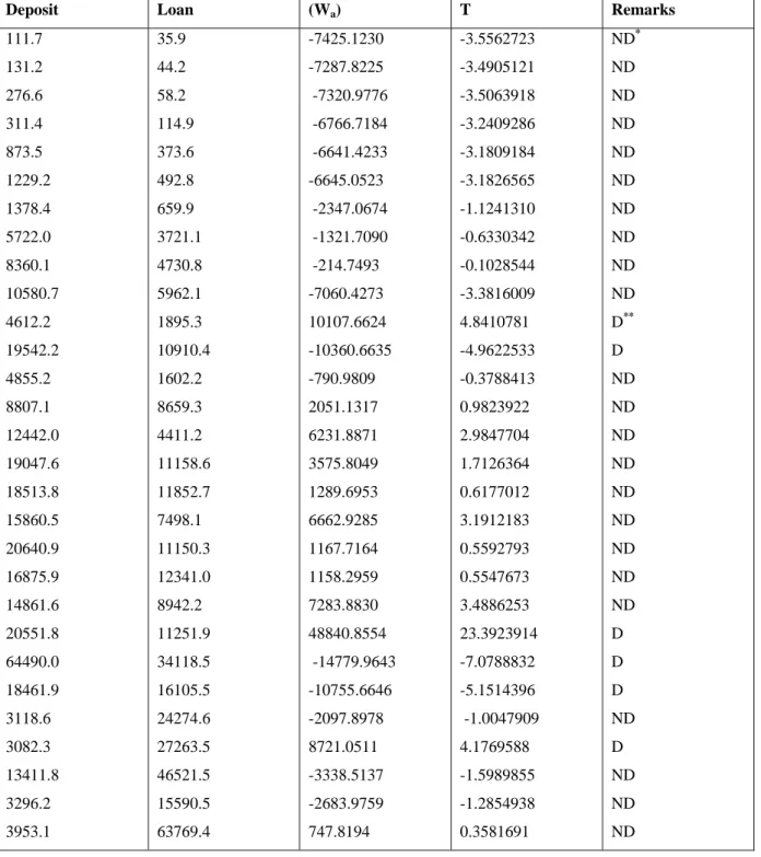
Table 3: Detection Performance of Additive Model on Deposit and Loan Data
Deposit Loan (Wa) T Remarks
111.7 131.2 276.6 311.4 873.5 1229.2 1378.4 5722.0 8360.1 10580.7 4612.2 19542.2 4855.2 8807.1 12442.0 19047.6 18513.8 15860.5 20640.9 16875.9 14861.6 20551.8 64490.0 18461.9 3118.6 3082.3 13411.8 3296.2 3953.1 35.9 44.2 58.2 114.9 373.6 492.8 659.9 3721.1 4730.8 5962.1 1895.3 10910.4 1602.2 8659.3 4411.2 11158.6 11852.7 7498.1 11150.3 12341.0 8942.2 11251.9 34118.5 16105.5 24274.6 27263.5 46521.5 15590.5 63769.4 -7425.1230 -7287.8225 -7320.9776 -6766.7184 -6641.4233 -6645.0523 -2347.0674 -1321.7090 -214.7493 -7060.4273 10107.6624 -10360.6635 -790.9809 2051.1317 6231.8871 3575.8049 1289.6953 6662.9285 1167.7164 1158.2959 7283.8830 48840.8554 -14779.9643 -10755.6646 -2097.8978 8721.0511 -3338.5137 -2683.9759 747.8194 -3.5562723 -3.4905121 -3.5063918 -3.2409286 -3.1809184 -3.1826565 -1.1241310 -0.6330342 -0.1028544 -3.3816009 4.8410781 -4.9622533 -0.3788413 0.9823922 2.9847704 1.7126364 0.6177012 3.1912183 0.5592793 0.5547673 3.4886253 23.3923914 -7.0788832 -5.1514396 -1.0047909 4.1769588 -1.5989855 -1.2854938 0.3581691 ND* ND ND ND ND ND ND ND ND ND D** D ND ND ND ND ND ND ND ND ND D D D ND D ND ND ND D** = Outlier detected ND* = No outlier detected
21
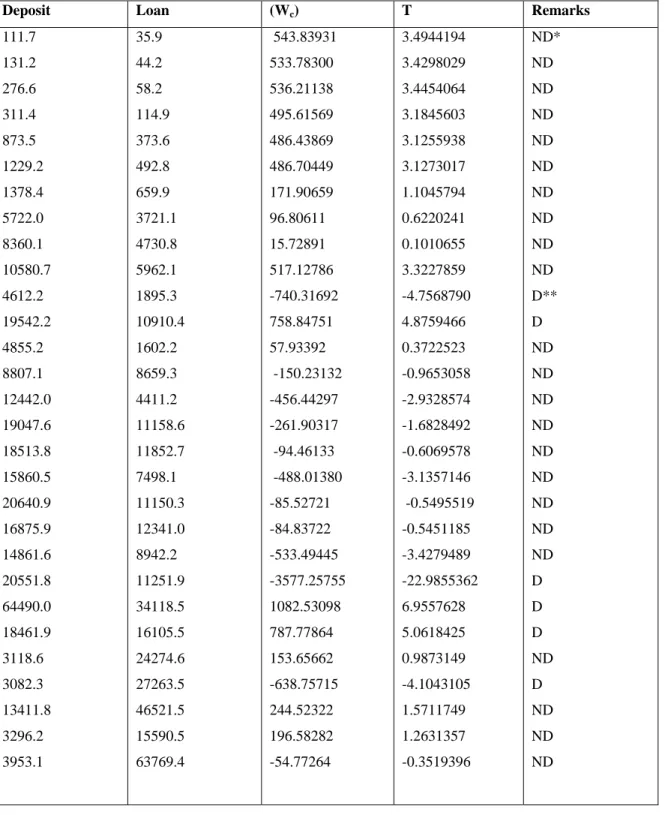
Table 4: Detection Performance of Convolution Model on Deposit and Loan Data
Deposit Loan (Wc) T Remarks
111.7 131.2 276.6 311.4 873.5 1229.2 1378.4 5722.0 8360.1 10580.7 4612.2 19542.2 4855.2 8807.1 12442.0 19047.6 18513.8 15860.5 20640.9 16875.9 14861.6 20551.8 64490.0 18461.9 3118.6 3082.3 13411.8 3296.2 3953.1 35.9 44.2 58.2 114.9 373.6 492.8 659.9 3721.1 4730.8 5962.1 1895.3 10910.4 1602.2 8659.3 4411.2 11158.6 11852.7 7498.1 11150.3 12341.0 8942.2 11251.9 34118.5 16105.5 24274.6 27263.5 46521.5 15590.5 63769.4 543.83931 533.78300 536.21138 495.61569 486.43869 486.70449 171.90659 96.80611 15.72891 517.12786 -740.31692 758.84751 57.93392 -150.23132 -456.44297 -261.90317 -94.46133 -488.01380 -85.52721 -84.83722 -533.49445 -3577.25755 1082.53098 787.77864 153.65662 -638.75715 244.52322 196.58282 -54.77264 3.4944194 3.4298029 3.4454064 3.1845603 3.1255938 3.1273017 1.1045794 0.6220241 0.1010655 3.3227859 -4.7568790 4.8759466 0.3722523 -0.9653058 -2.9328574 -1.6828492 -0.6069578 -3.1357146 -0.5495519 -0.5451185 -3.4279489 -22.9855362 6.9557628 5.0618425 0.9873149 -4.1043105 1.5711749 1.2631357 -0.3519396 ND* ND ND ND ND ND ND ND ND ND D** D ND ND ND ND ND ND ND ND ND D D D ND D ND ND ND D** = Outlier detected ND* = No outlier detected
22
Table 5: Summary of Outlier Detection of the Two Models on Deposits and Loan Data
Model No of outliers detected Convolution 6 Additive 6 **Innovation 5 **Multiplicative Nil **Source: [19] 4. Discussion of Results
From the analyzed simulated data with varying sample sizes of 10, 50, and100, the average percentage rates of outlier detection for AO and CO are 68% and 100% respectively of the injected outliers. From the result, CO was consistent in outlier detection as the sample size increases. Comparing the performance of these two newly derived models with the existing models, the CO outperformed both Multiplicative and Innovative models that have average detection rate of 86.7% and 21.7% respectively for the simulated data.
For the real data set of Deposit and Loan, 6 outliers were equally detected by the two models when we consider the case of deposit depending on loan. The two derived outlier-generating mechanisms were able to detect potential outlier independently in multivariate time series. However, comparing the performance of these models with the existing ones, AO and CO detected 6 outliers while Innovative model was able to detect 5 but Multiplicative model detected no outlier as a result of non-multiplicative nature of data. [19].
In summary, CO was found to be most sensitive to outliers for the simulated data sets as the sample increases and also for the real data. When compared also with the existing models, CO has been found to be most efficient with minimum standard error of the estimate and is therefore recommended for outlier detection in multivariate time series data.
5. Conclusion
This work was undertaken to develop test statistic for detecting outliers assuming two different outliers generating mechanisms in multivariate time series models. In line with the main objective of this paper, the test statistics were derived for each generating mechanism namely; the Additive and Convolution models. The model with greatest detective power in terms of their sensitivity to the number of outliers detected by applying the models to both simulated and a pair of real data were determined. All these were achieved using theoretical and analytical methods. The convolution model was found to be most sensitive to outlier detection when compared with existing models, it is therefore recommended for outlier detection in multivariate time series.
23
References
[1] Z. Azami, A. Ibrahim and S. Mohd. “Detection Procedure for a Single Additive Outlier in Bilinear Model.” Journal of Pak. Stat. Oper. Res. Vol. No 1 PP. 1-5, 2007.
[2] R. Baragona and F. Battaglia. “Outlier Detection in Multivariate Time Series by Independent Component Analysis.” Neutral Computation, 19:1962-1984.
[3] R. Baragona, F. Battaglia and C. Alzini. “Genetic Algorithms for the Identification of Additive and Innovational Outliers in Time Series” Computational Statistics and Data Analysis. 30,147,2001.
[4] V. Barnett. “The study of outliers: Purpose and Model.” Applied Statistics, 27(3), 242–250,1978.
[5] V. Barnett and T. Lewis. Outlier in Statistical Data. John Wiley & Sons U. K. 1994.
[6] G.E.P. Box, G.M. Jenkins and G. Reinsel. Time Series Analysis: Forecasting and Control,3rd Ed., New Jersey: Prentice-Hall,1994.
[7] K. Chaloner and R. Brant. “A Bayesian Approach to Outlier Detection and Residual Analysis.” Biometrika, 25, 651 – 660,1988.
[8] I. Chang, et. al. “Estimation of Time Series Parameters in the Presence of Outliers” Technometrics, 3, 193.204,1988.
[9] C. Chen and L.M. Liu. “Joint Estimation of Model Parameters and Outlier effects in Time Series.” Journal of the American Statistical Association, 88, 284 – 297,1993.
[10] D. Cucina, A.Di Salvatore and M. Protopapas. ‘’Meta-heuristic Methods for Outliers Detection in Multivariate Time Series.’’ Comisef working paper series, 003,270,2008
[11] A.J. Fox. “Outliers in Time Series.” Journal of the Royal Statistical Society. B34: 350 – 363,1972
[12] P. Galeano, D. Pena and R.S. Tsay. “Outlier Detection in Multivariate Time Series via Projection Pursuit.” Working paper 0-42. Statistics and Econometrics Series II, Dept. De Estadistica, Universidad Carlos III de Madrid,2004
[13] J. Helbling and R. Cleroux. “On Outlier Detection in Multivariate Time Series.” Mathematical Volume 34, Number 1, pp. 19-26,2009.
[14] A. Kaya. “Modelling Outlier Factors in Data Analysis.” Advances in Information Systems, LNCS 3261, 88 – 95,2010.
24
Statistics – Theory and Methods, 16(12): 3701 – 3714,1987.
[16] G.M. Ljung. “On Outlier Detection in Time Series.” J. R. Statist. Soc. B. 55 No. 2, 559 -567,1993.
[17] C.R. Nelson, and C.L. Plosser. “Trends and Random Walks in Macroeconomic Time Series.” Journal of Monetary Economics, 10, 139 – 162,1982.
[18] D. Olivier and C. Amelie. “The Impact of Outliers on Transitory and Permanent Components in macroeconomic Series.” Economic Bulleting, Vol. 3, No 60 PP 1 – 9,2008.
[19] O. Olufolabo, O.I. Shittu and K.A. Adepoju. “Performance of Two Generating Mechanisms in Detection of Outliers in Multivariate Time Series.” American Journal of Theoretical and Applied Statistics.5(3), 115-122,2016.
[20] A. Pankratz. Forecasting with Univariate Box-Jenkins Models: Concepts and Cases, New York: John Wiley and Sins,1983.
[21] A. Pankratz. “Detecting and Treating Outliers in Dynamic Regression Models.” Biometrika,80, 47-54,1993.
[22] D. Pena and G.E.P. Box. “Identifying a Simplifying Structure in Time Series.” Journal of the American Statistical Association, 82, 836-843,1987.
[23] S. Ruey and R.S. Tsay. “Outliers, Level Shifts, and Variance Changes in Time Series.” Journal of Forecasting, Vol. 7, I-20 Department of Statistics, Carnegie Mellon University, U. S.A,1988.
[24] D.K. Shangodoyin. “On the Specification of time series Models in the Presence of Aberrant Observations”. Ph.D. Thesis in the Dept. of Statistics, Univ. of Ibadan,1994.
[25] I.O. Shittu and D.K. Shangodoyin. ‘’Detection of Outliers in Time Series Data: A Frequency Domain Approach.’’ Asian Journal of Scientific Research 1, (2) 130-137,2008.
[26] I. O. Shittu. “On Performance of Some Generating Models in Detection of Outliers Under Classical Rule.’’ M.Phil. Thesis. Dept. of Statistics, Univ. of Ibadan,2000.
[27] C. Sims. “Macroeconomics and Reality.” Econometricsa 48 (1), 11-46, JSTOR 112017,1980.
[28] R.S. Tsay. “Time Series Model specification in the Presence of Outlier.” Jour. Amer. Stat. Asso. 81, 132 – 141,1986.
[29] R.S. Tsay. “Outliers, Level Shifts and Variance Changes in Time Series.” Journal of Forecasting, 7, 1-20,1988.
25
[30] R.S. Tsay, D. Pena and A.E. Pankratz. “Outliers in multivariate time series.” Biometrika, 87, 789-804,2000.
[31] X.Wang. “Two-Phase Outlier Detection in Multivariate Time series.” Fuzzy Systems and Knowledge Discovery, Eighth International Conference. Vol.3,2011.
[32] Ji. Yanjie et al. (2013). “Detection of Outliers in a Time Series of Available Parking Spaces.” Mathematical Problems in Engineering, Volume 2013: 1-12,2013.