University of Nebraska - Lincoln University of Nebraska - Lincoln
DigitalCommons@University of Nebraska - Lincoln
DigitalCommons@University of Nebraska - Lincoln
Presentations, Working Papers, and Gray
Literature: Agricultural Economics Agricultural Economics Department October 2008
2007 Farm Bill Forums: Issues and Options
2007 Farm Bill Forums: Issues and Options
Bradley Lubben
University of Nebraska-Lincoln, [email protected] Samuel Funk
Kansas State University Troy J. Dumler
Kansas State University
Follow this and additional works at: https://digitalcommons.unl.edu/ageconworkpap
Part of the Agricultural and Resource Economics Commons
Lubben, Bradley; Funk, Samuel; and Dumler, Troy J., "2007 Farm Bill Forums: Issues and Options" (2008). Presentations, Working Papers, and Gray Literature: Agricultural Economics. 24.
https://digitalcommons.unl.edu/ageconworkpap/24
2007 Farm Bill Forums
2007 Farm Bill Forums
Issues and Options
Issues and Options
A Series of Farm Bill Educational Meetings for
Producers and Interested Policy Stakeholders
in Kansas and Nebraska
Kansas
Sabetha -- February 20
Emporia -- February 21
Hays -- February 22
Nebraska
Scottsbluff -- February 26
Cozad -- February 27
Hastings -- February 28
Columbus -- March 2
Several policy experts from both the Univer-sity of Nebraska-Lincoln and Kansas State University will be involved in the meeting series:
• Paul Burgener
Ag Economics Research Analyst Panhandle Research and Extension Center
University of Nebraska-Lincoln P: 308.632.1241
• Troy Dumler
Extension Agricultural Economist Kansas State University
Southwest Research and Extension Center
P: 620.275.9164 E: [email protected]
• Sam Funk
Agricultural Policy Specialist
Department of Agricultural Economics Kansas State University
P: 785.532.1506
• Brad Lubben
Extension Public Policy Specialist Department of Agricultural Economics University of Nebraska-Lincoln
P: 402.472.2235 E: [email protected]
Agenda
9:30 a.m. Registration
9:45 a.m. Introductions and Com-ments
10:00 a.m. Setting the Stage for the Farm Bill Debate
Exploring the Rationale for Farm Programs Understanding the Alter-natives for the Farm Bill Alternative I: Existing Commodity Programs and Potential Adjust-ments
12:00 noon Lunch
1:00 p.m. Alternative II: Revenue Safety Net
Alternative III: Green Pro-grams for Conservation and Bioenergy
2:00 p.m. Group Discussions Wrap-up Discussion/ Panel Discussion with Presenters
University of Nebraska-Lincoln Extension is a Division of the Institute of Agriculture and Natural Resources at the University of Ne-braska-Lincoln cooperating with the Counties and the United State Department of Agriculture.
1
The 2007 Farm Bill: Drivers of the Debate
Bradley D. Lubben Extension Public Policy Specialist
University of Nebraska-Lincoln
Samuel M. Funk Agricultural Policy Specialist
Kansas State University
Troy J. Dumler
Extension Agricultural Economist Kansas State University
The debate on the 2007 Farm Bill has begun in earnest in Washington. The new Congress has already convened several hearings on farm policy issues, including energy and conservation. The Administration has just released its policy recommendations for the new farm bill, opening up further discussion that will grow over the coming months. The current farm bill, passed in 2002, runs through September 2007 and includes programs covering the 2007-2008 crop year. Before it expires, Congress will need to reconcile the current discussion and debate and either pass a new farm bill or an extension of the current one. While the discussion and development of the new farm bill will be played out over the coming months, it is important to remember several fundamental factors that drive the debate. Drawing from an old adage, “farm bills are always a product of their times.” While the exact setting changes from farm bill to farm bill, the same key factors continue to drive the debate. The economic setting, the budget setting, the trade arena, and the political climate all influence the development of each farm bill. Understanding each of these drivers is a fundamental part of understanding the potential new farm bill.
Economics
The economic setting heading into the 2007 Farm Bill is clearly different than it was in 2001 when the 2002 Farm Bill was developed. In the four years leading up to the 2002 Farm Bill, U.S. net farm income less government payments averaged just over $30 billion (see Figure 1) and was supplemented with nearly $20 billion annually in government payments, including emergency assistance from Congress. The 2002 Farm Bill debate focused in part on the size of the farm income safety net and the calls to formalize the emergency assistance into a basic part of the safety net. At the time, the counter-cyclical payment program was advertised as exactly that.
In early 2007, the economic setting is very different. Coming off of record farm income levels in 2004 and 2005 above $70 billion (see Figure 1), farm income levels moderated in 2006 to $61 billion. There have also been concerns about higher energy costs taking several billion dollars additional dollars out of net farm income. But, the higher energy prices have also supported the rapidly-developing biofuels industry, creating new demand for agricultural commodities, particularly corn. The resultant increase in the price of corn and other commodities has sparked a surge in crop profitability and the first forecast of 2007 net farm income just released from USDA projects a rebound in U.S. net farm income to nearly $67 billion. If the projections hold, the 2004-2007 period will represent the strongest U.S farm income performance on record (in nominal terms). While government payments continue to be a significant share of farm income
$0 $10 $20 $30 $40 $50 $60 $70 $80 $90 1970 1975 1980 1985 1990 1995 2000 2005 B illions
Net Farm Income (Less Govt Pay) Government Payments
at an estimated $16.5 billion annually over the same time period, the strength of the farm economy changes the debate from one about the size of the safety net to one about the shape of the safety net. Already, the current higher grain price and economic outlook for the U.S. agricultural sector has variously led to calls 1) to end farm income support programs as unnecessary, 2) to strengthen programs and raise the level of the safety net under current higher prices, 3) to shift the program from one based on prices to one based on revenue, or 4) to simply extend the current safety net as a cost-saving option in light of other concerns in the budget and trade arena.
Budget
The budget setting is also very different now than it was in 2001. In 2001, the debate was about how to allocate an additional $70 billion in baseline spending for agriculture out of a growing federal budget surplus. Since then, the focus has shifted to the size of the federal budget deficit (see Figure 2) and the possible spending cuts to reduce the deficit. The deficit of $248 billion in fiscal year 2006 (matched up in the graph as the lead-in year of the 2007 Farm Bill debate) is the largest ever amidst a farm bill debate. In this budget climate, the President
has proposed agricultural spending cuts in each of his past three budget requests, including the fiscal year 2008 budget request just released in early February. The Deficit Reduction Act of 2005 did make several cuts in farm program spending, including cuts to conservation, rural development, and research and delayed part of the direct (fixed) payments to producers.
While these initial cuts signal continued pressure on farm program spending, there are several caveats to temper the budget concerns. First, farm bills almost always have been debated in times of federal budget deficits. Only two farm bills in the last 40-plus years (1970 and 2002) were debated in the presence of a budget surplus. In addition, the current deficit represents only 1.9 percent of the nation’s GDP (right axis in graph in Figure 2) and is much lower in real terms (constant dollars) than the deficit at the time of most farm bill debates since the mid-1970s.
Another point of emphasis is that current farm programs are actually costing less than expected. Due to higher crop prices and future price projections, spending on farm commodity programs is several billion below original budgeted levels. In the new baseline budget estimates released in January by the
Congressional Budget Office (CBO), 10-year spending projections for mandatory farm support programs are $35 billion less than the 10-year projections issued in January 2006. This reduced spending does not technically count as savings to be allocated elsewhere, but it does change the political climate in which federal budget decisions will be made.
These budget decisions will in fact represent the first test of future policy directions. While the agricultural committees have jurisdiction over the authorization of new farm bill, the budget committees will determine the dollar limit to put on that authority. The baseline spending projections in March 2007 will represent the starting point for discussions. While the higher prices and reduced spending projections may suggest the possibility of additional baseline allocations for agriculture, Congress must also deal with the “Pay-As-You-Go” (PAYGO) budget rule adopted in the U.S. House of Representatives. These rules stipulate that any
-500 -400 -300 -200 -100 0 100 200 1965 1970 1973 1977 1981 1985 1990 1996 2002 2007
Farm Bill Cycle Year
$ B illio n -5 -4 -3 -2 -1 0 1 2 % of GD P
Budget Balance - $ Billion (left) Budget Balance - % of GDP (right) Figure 2. Federal Budget Projections (CBO)
3
bill that offers provisions increasing spending from CBO budget baseline estimates be offset by spending cuts (or tax increases) in other provisions.
The budget setting presents a difficult outlook for programs looking for increased funding in the 2007 Farm Bill. The deficit and the PAYGO rules both suggest a difficult challenge for any proposed increases in baseline funding for new or existing programs. At the same time, the reduced baseline projections for spending under the commodity programs means the overall size of the farm program pie could be smaller than most groups expected, leaving less opportunity for political and budget tradeoffs of one program for another.
Trade
The trade setting is dominated at present by two key questions. Will the WTO Doha Round negotiations break out of its current stalemate and move toward an agreement? Will the U.S. be subjected to repeated challenges of its farm programs under the conflict resolution process of the existing trade agreement? Both of these questions may point toward necessary reforms in U.S. farm programs.
The WTO Doha Round negotiations have been a slow, complex process since they officially began in 2001. In a framework agreement in July 2004, WTO member nations agreed to do three things in regard to agriculture: 1) increase market access (i.e. reduce tariffs and barriers that discourage imports), 2) reduce trade-distorting domestic subsidies, and 3) eliminate export subsidies. The difficulty in reaching agreement revolves around how these framework objectives are to be met. How much will tariffs and domestic subsidies be reduced? What is the time frame for these reductions? The goal was to work these details out at a WTO summit in Hong Kong in December 2005. When that meeting failed to reach
consensus, the talks stretched into 2006 and continued until July, when the WTO Director-General Pascal Lamy suspended the negotiations, calling for a period of “time-out” to allow WTO members to reassess their negotiating positions.
Table 1. World Trade Organization Negotiations and Agricultural Issues Post Hong Kong.
Export Competition Domestic Supports Market Access
(direct subsidies on exports) (domestic subsidies with effects on production and trade)
(domestic barriers restricting imports)
Agreement to phase out export subsidies by 2013
-includes direct export subsidies -includes subsidy portions of export credit programs
Agreement to eliminate cotton export subsidies in 2006
Disciplines on food assistance and establishment of “safe box” for bona fide food aid
Reduction of aggregate measures of support (AMS) across three bands (“Amber Box” and “Blue Box” programs) -higher cuts for higher bands of current spending
-Europe likely in highest band -Japan and U.S. likely in second band
-Bands, cuts, and schedule for cuts not yet developed
No disciplines discussed on “Green Box” programs
Elimination of 97 percent of existing tariff lines on imported products from least-developed countries
Reduction in tariff rates across four bands
-higher cuts for higher bands of current tariff rates
Flexible terms for “sensitive” products
-limited number of “sensitive products” not confirmed
Since July 2006, informal discussions have continued at various venues, but to date, no breakthrough compromise agreements have been announced. While the U.S. Trade Representatives have offered proposals to reduce trade-distorting domestic farm program payments to secure progress from the European Union (EU) and other in opening markets, the EU and numerous developing countries have insisted that the United States must improve its offer to reduce domestic subsidies before they will increase market access. At the same time, various U.S. policymakers and interest groups have argued that it is the EU and the other counties that need to make a better offer of market access in the WTO. While the WTO negotiations could continue almost indefinitely with little progress, the calendar does present two issues in the United States to prod the negotiations forward. The first is the President’s trade promotion authority (TPA). This authority to negotiate trade agreements that are subject to ratification by Congress without amendment expires in July 2007. If TPA expires and is not renewed, as seems likely in the current Congress, then the President’s ability to negotiate any trade agreement is severely restricted. TPA requires any trade agreement to be voted on as is without amendments. Not having TPA would mean Congress might add several amendments to the implementation of any WTO agreement, essentially scuttling the agreement as written and eliminating the President’s ability to negotiate in good faith.
The above discussion notes that a WTO agreement could demand changes in U.S. farm programs. At the same time, the failure of a WTO agreement could also lead to changes in U.S. farm programs. The United States has already been found in violation of WTO rules as agreed to in the previous round of trade negotiations, the “Uruguay Round Agreement on Agriculture.” Under that agreement the United States and other countries subsidizing agriculture made commitments on reducing the amount of subsidies and limiting the total spending on trade-distorting programs. Based on the rules of that agreement, Brazil filed suit against the United States in the WTO, claiming that total subsidies on U.S. cotton exceeded the allowed limits set forth in the Uruguay Round. The WTO found in favor of Brazil and ruled that the United States must change certain cotton programs, or face retaliatory damages of several billion dollars. There are some important implications of the Brazilian cotton case for U.S. farm programs. First, it was determined by the WTO that the U.S. direct payment program is not a “green box” (minimally trade distorting and unlimited) program. Rather, it is an “amber box” (trade distorting and limited) program that has more significant trade distorting aspects because of a restriction on planting fruits and vegetables on contract acres receiving a direct payment. This issue will have to be addressed by Congress should they determine it important to make direct payments a “green box” program.
Second, the United States has thus far made some policy changes for cotton, including the elimination of the Step 2 program and the elimination of violating portions of the export credit programs. But, the United States has not made any adjustments to the marketing loan and counter-cyclical payment programs also found to be in violation of support limits. As a result, Brazil has filed a follow-up complaint arguing that the United States has only partially implemented policy changes required to comply with the ruling and demanding either compliance or the right to enact retaliatory measures. Congress will have to address these issues as well within the scope of the farm bill deliberations.
Third, the model of the Brazilian cotton case can be readily translated to other program commodities, given the same set of farm policy tools. At the moment, Canada has initiated consultations with the WTO in complaint of U.S. corn subsidies, with several other countries joining the consultations. If a new WTO agreement is not achieved, these disputes and others could become more commonplace and result in piecemeal challenges and changes in U.S. farm programs over time.
Between the trade negotiations on a new agreement that would demand farm spending reforms and the potential piecemeal changes that could occur in response to WTO complaints in the absence of a new agreement, it appears that changes are coming. However, the changes do not necessarily dictate the end of farm programs. They simply demand at least some shift to programs that are more acceptable in the
5 Politics
Finally, one cannot prepare for the next farm bill debate without noting the role of politics. An often-used saying is that “politics always trumps economics” and that is certainly true with the farm bill. Although the economics of farm income, federal budgets, and trade agreements will certainly push some of the debate, the farm bill will eventually largely be a product of the political environment in which it is created. And that environment has changed substantially since the last farm bill was completed in 2002.
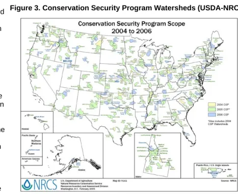
With the November 2006 elections, Democrats regained control of both the Senate and the House of Representatives, meaning new committee chairs assumed leadership in January, just in time to develop the new farm bill. The shift from two Republican committee chairs to two Democratic committee chairs may bring with it a larger focus on certain specific policy issues such as the Conservation Security Program and the role of payment limits, two issues that have the interest of Senator Tom Harkin of Iowa, the new Senate agricultural committee chair.
However, it is worth remembering another old saying that “farm bills are generally more parochial than they are partisan.” With Representative Collin Peterson leading the House agriculture committee, the new Congress has two agriculture committee chairs from the Upper Midwest whereas the previous Congress had two chairs from the South. Regional differences in farm program spending, basic commodity issues, and conservation targets could lead to challenging committee work that is more split along regional lines than political lines.
While the formal change in Congress is significant, it is also important to recognize the emerging presence of several farm bill interest groups outside the traditional farm, commodity, and agribusiness sector. For more than 30 years, the development of each farm bill has been a comprehensive, coalition-supported process. And yet, the traditional groups within production agriculture clearly played the role of lead partner. Increasingly, that model has been challenged by other interest groups.
Conservation programs have grown substantially in recent years. In fact, the 2002 Farm Bill has been widely reported as the “greenest” farm bill to date, with nearly $3 billion in annual conservation program spending for programs like the Conservation Reserve Program (CRP), the Environmental Quality Incentives Program (EQIP), and the new Conservation Security Program (CSP). And yet, conservation spending has also been a regular target for Congress when spending cuts have been required to offset disaster payments or satisfy budget reconciliation requirements.
Conservation and environmental groups have placed an increased emphasis on securing additional funding for conservation programs. One group, the Environmental Working Group, utilized the public availability of program payment data and published a widely-referenced database of government payments. This database has substantially shifted the debate over conservation spending from “How much money for conservation?” to “Why so much money for commodities?”
Similar strategies are appearing in other special interest areas as well. Food nutrition and assistance groups have historically been the “urban” partner to the “rural” production agriculture sector in building political support for a comprehensive farm bill. But, groups in this area are looking more to their own programs, questioning why the United States is subsidizing the production of food and feed grains and not “more nutritious” fruits and vegetables. And in the rural development area, groups are looking at the role of bioenergy as a new driver of economic activity across the rural United States.
While the other interests groups have been honing their message and increasing their efforts, the farm, commodity, and agribusiness interests are still central to the debate. The political battle has largely been played out thus far as other interests fighting for a larger piece of the total farm bill spending pie, each hoping to take some of the current share going to traditional commodity programs. With the early expectations of cuts for trade or budget reasons, coupled with potential savings from payment limit changes, there were hopes for substantial funds to be freed up for other programs.
However, there are some limits to that political strategy. First, as noted in the budget setting, the current projections for higher prices mean the baseline spending projections for existing commodity programs are down substantially. This simultaneously means that there is less baseline to potentially reallocate to other programs and that maintaining the existing commodity programs is suddenly more feasible in terms of both trade and budget constraints. Another political factor to consider is that the farm commodity programs remain a core part of the farm bill. If the core agricultural interests are diminished in the farm bill process, the overall driving force to pass a farm bill could be diminished as well. Shifting the major focus of the farm bill away from production agriculture could just as easily lead to no farm bill and no major reauthorization as it could to an increased role for the other program areas.
Conclusion
Reflecting on the four factors driving the debate - economics, budget, trade, politics - the farm bill
development will continue to be a complex and challenging process. The various competing interests have yet to battle over budget allocations and only then will they be able to fully engage in the battle over program alternatives. The real farm bill debate is only now getting started, with Congressional hearings underway and the Secretary’s farm bill recommendations now out. Congress has already hosted the Secretary for testimony on the Administration’s farm bill recommendations and will likely convene several more hearings to receive testimony and recommendations. Then Congress will begin the work of
developing farm bill language in the agricultural committees and moving it toward final passage. Discussions in committee and on the floor of Congress could well last through the summer of 2007 or beyond, making for an interesting several months ahead.
Historical Rationale for Farm Programs
Troy J. Dumler
Extension Agricultural Economist K-State Research and Extension
Supporters of U.S. farm programs offer many justifications for the current and future use of farm programs. The most common of these justifications include: saving the family farm, supporting rural communities, providing a cheap food supply, maintaining the environment, and competing with large agribusinesses and subsidizing countries. A recent survey on preferences for the 2007 Farm Bill indicates that U.S. producers still value these justifications for farm subsidies (Farm Foundation). Oftentimes these
justifications are cited by supporters and treated as fact. But are they fact? Following is a discussion of the primary historical arguments for farm subsidies.
Saving the Family Farm
The rational for saving the family farm through farm subsidies is both emotional and economic. The emotional aspect has its roots in the founding of the United States. At the time of its independence from Great Britain, the United States was essentially a nation of farmers. Prominent founding fathers like George Washington and Thomas Jefferson were farmers themselves. Jefferson’s vision for the United States, later termed the Jeffersonian democracy, was “a nation of landowning farmers living under as little government as possible.” (Worldbook.com) As the nation expanded westward, so did agriculture— fulfilling Jefferson’s vision, at least in part.
The image of a nation of small farmers still resonates. Certainly, small farm advocacy groups promote such a system. The fact that 42% of the 2.1 million farms in the U.S. are residential or lifestyle farms (Hoppe and Banker, p.11), indicates that many people still value aspects of the agricultural lifestyle. Likewise, the fact that U.S. taxpayers have been willing to subsidize farmers at an average rate of $17 billion over the last 10 years
(USDA-ERS, 2006a) suggests that they, at least to a certain extent, value Jefferson’s vision as well.
Farm and Non-farm Household Income
Current farm subsidies originated in Franklin Roosevelt’s New Deal legislative package in 1933. At that time, average farm household income was about half of that of non-farm households (Jones, et al.). Also, in 1930, 21.5% of the U.S. workforce was employed in production agriculture that contributed 7.7% of the total U.S. GDP. With a large
workforce earning income half that of their non-farm counterparts, the federal
government felt compelled to provide assistance to farmers in the form of price supports and supply management.
Today, the situation in agriculture is much different. In 2000, only 1.9% of the U.S. workforce was employed in production agriculture, and agriculture contributed only 0.7%
of U.S. GDP in 2002 (Dimitri, et al.). Moreover, farm households now routinely earn more than non-farm households. Figure 1 shows farm and non-farm household income in the U.S. from 1960-2004. After reaching a level basically on par with non-farm income in the 1960s, farm household income was 33% higher than non-farm income in 2004 (Jones, et al). Based on these numbers alone, it would be hard to justify subsidizing farms on the basis of disparities in income as was originally the case when farm programs were first instituted in 1933.
U.S. Farm and Nonfarm Household Income
0 20,000 40,000 60,000 80,000 100,000 1960 1970 1980 1990 2000 $/ H o u se h ol d
Farm Household Inc Nonfarm Household Inc
Figure 1
Supporters of farm subsidies may make the argument that farm income would not be greater than or equal to non-farm income without subsidies. If one considers that
government payments contributed 30.6% of net farm income from 2000-06 (USDA-ERS, 2006a), that argument would seem to have some merit. However, one must also
remember that not all government payments go to farmers. Since commodity program payments are tied to land, landowners benefit as well.
Farm subsidy proponents will also often point out that the majority of farm household income comes from non-farm sources. That is certainly true when household income is averaged across all farms. However, when broken out by USDA farm typology class, not all farms receive the majority of household income from non-farm sources. Table 1 shows household income from farm and non-farm sources by USDA farm typology group in 2004. Rural residence farms, which include limited-resource,
residential/lifestyle, and retirement farms, had an average household annual income of $75,316. Non-farm sources were responsible for 100% of total household income for these farms. Because 42% of all farms are residential/lifestyle farms, which claim a primary occupation other than farming, it is not surprising that the average farm would earn a high percentage of household income from non-farm sources. But as table 1 also indicates, commercial farms (i.e., farms with sales over $250,000) earn over 75% of household income from farm sources. Basically this leads to the warning that people should be careful not to draw too strong of conclusions when comparing farm household income to non-farm household income.
3
Table 1. Household Income from Farm and Non-farm Sources by USDA Farm Typology. Farm Typology Group No. of Farms Total Farm Household Income Income from Farm Sources Income from Non-farm Sources % from Farm Sources Rural Residence 1,373,956 $75,316 $-76 $75,391 -0.1 Intermediate 529,071 $64,789 $12,240 $52,549 18.9 Commercial 157,795 $191,115 $145,080 $46,035 75.9 All 2,060,822 $81,480 $14,201 $67,279 17.4 Source: USDA-ERS, Agricultural Resource Management Survey, 2004.
Equity of Farm Income Support
While the goal of saving the family farm may be noble from a social standpoint, there are questions as to whether the current farm income support programs are meeting that objective from an economic standpoint. These questions revolve around two primary issues. First, are government payments distributed equitably across the farm sector? Second, is profitability enhanced for farms that receive government payments?
According to data from USDA, only 39% of U.S. farms received government payments in 2003 (Hoppe and Banker, p. 25). Of those farms that received farm subsidies, 66% of total payments went to five commodities: corn, cotton, wheat, soybeans, and rice (USDA, CCC Net Outlays by Commodity and Function). Because medium, large and very large farms (those farms with annual sales greater than $100,000) have a higher percentage of farms that specialize in cash grains and other field crops that receive subsidies, they receive a higher percentage of payments (figure 2). This, in turn leads to criticisms that “large farms get all the payments”. However, the fact that large commercial farms receive the bulk of government payments has less to do with large farms abusing subsidy
programs to the detriment of small farms (as some try to make the case), than it does with the structure of the farm programs themselves. If the goal of U.S. farm income support is to save the family farm, and between 35 to 41 percent of small farms (limited-resource,
Share of farms, value of production, and government payments by farm typology group, 2003
0 10 20 30 40 50 Ltd. Reso urce Retir e-men t Lifes tyle Small -low sales Small -med ium sa les Larg e Very larg e No n-family P e rc en t Farms VOP Govt Pmt Figure 2
retirement, residential/lifestyle, and farming-occupation/low sales farms) produce beef, should beef producers not receive income supports as well? Given the current structure of farm programs and the equity issue created from tying farm program payments to specific commodities, the argument that farm subsidies help save the family farm is debatable.
Nevertheless, government payments have contributed a significant portion of net farm income over the last two and one half decades (figure 3). But as previously mentioned, not all the benefits of government payments go to farmers, as a portion of those benefits gets capitalized into land values. This reality has two ramifications. First, it demonstrates that family farms are not the only beneficiaries of farm subsidies. Second, it indicates that as farm income would decline from a reduction or elimination of government payments, farm asset and equity values would also decline.
A study by Kastens and Dhuyvetter estimated that average cropland values by state would fall by 2.3% to 40.8% if government payments were eliminated. Certainly, a reduction in land values of that magnitude could have a devastating effect on the financial viability of many farms. The estimated decline in land values, however, assumes that 100% of government payments are capitalized into land. In reality, government payments are not likely to be fully capitalized into land values.
The greatest challenge facing most commercial farms in the U.S. is variability of income. Figure 3 shows U.S. aggregate net farm income (NFI) and direct government payments from 1997-2006. Over that timeframe, NFI averaged $57.2 billion per year, with a range from $40.2 billion in 2002 to $85.4 billion in 2004. Government payments, as previously noted average $17 billion during those same years, accounting for 31% of NFI. Certainly, farm income is variable and government payments have contributed a significant share of income over the last 10 years. However, the aggregate U.S. data actually mask income variability and the importance of government payments associated with some regions and commodities. Even though not all farms will become unprofitable if government
payments are eliminated, it is also important to realize that in some years, in some regions, government payments contribute a large portion of NFI. Undoubtedly, an
U.S. Net Farm Income and Direct Government Payments
0 20 40 60 80 100 1996 1997 1998 1999 2000 2001 2002 2003 2004 2005 B illio n $ 0 10 20 30 40 50 P e rc en t GP NFI GP % of NFI Figure 3
5
immediate elimination of farm programs would have severe consequences for farmers and rural communities historically dependant on those programs. How farms manage the variability of income, especially if farm programs were to be reduced or eliminated, will be a big factor in determining the long-term success of a farm. Because the U.S. has chosen to help some farmers manage risk through farm supports does not imply that there are not other means to manage financial risk.
Supporting Rural Communities
Oftentimes the words “farm” and “rural” are used interchangeably. In the past, such use may have been reasonable. Today, however, that likely will not be accurate. According to information in USDA’s 2007 Farm Bill Theme Paper on Rural Development, “less than 10 percent of rural people currently live on a farm and only 6.5 percent of the rural workforce is directly employed in farm production.” That compares to 40 % of the rural population living on farms, with 33 percent of the rural workforce directly employed in agriculture in 1950. Although only 10% of the rural population currently lives on farms, 20% of rural counties are classified as farm-dependant (greater than 20% of county personal earnings come from farming). Of those counties, 78% had a population loss from 2000-2005. The poor economic performance of these farm-dependant counties and subsequent population losses have led to subsidies being viewed as a remedy for rural America.
By supporting farm income through farm programs, proponents of farm subsidies argue that these programs help save rural communities as well. The logic of this argument is straightforward. If farmers make more money, that money will then be spent in the community—stimulating economic growth. In other words, if farmers are doing well, then rural communities will do well. If one follows the logical progression of this argument then one would expect rural communities that receive high amounts of farm subsidies to perform well economically. However, a recent study by the Center for the Study of Rural America of the Federal Reserve Bank of Kansas City suggests that such an argument may not hold. Instead of growing, U.S. counties that were most dependent on farm payments relative to the local economy actually experienced job and population growth rates lower than counties less dependent on payments. As the article points out though, it is possible that economic performance would have been even worse without the payments.
The question that naturally comes to mind when seeing such results is: Why do most counties that are most dependent on farm payments perform worse than other rural counties? There are several possible explanations. First, the government payments themselves may have a negative impact. Programs such as the marketing loan program encourage production above market clearing levels. That, in turn, keeps prices lower than they would otherwise be without the loan program. In such a scenario, the low cost producer will be most profitable. Moreover, low cost producers have advantages over their high cost counterparts in lowering costs. Low cost producers can afford to outbid other producers in acquiring land, which enables them to get larger and spread fixed assets such as machinery over more output. This process encourages farms to get larger in order to be profitable. Since there is a limited amount of farmland available, not all
farms can expand to remain profitable. Consequently, farms go out of business and the economic viability of communities suffers.
A paper by McGranahan and Beale offers some other possible explanations for rural population loss. Although poverty rates declined in 85% of rural counties in the 1990s, many farm-dependent counties continued to experience population loss. However, it is not necessarily the economic viability of agriculture in farm-dependent counties that is causing population loss. As McGranahan and Beale state:
“what distinguishes farm-dependent counties from other rural counties is less the presence of farming than the absence of nonfarm activities. Farm-dependent counties are more likely to be remote from metro areas, to have low population density, and to lack natural amenities. These characteristics, which discourage other types of development, account for much of the population loss in farm-dependent counties.”
Because rural residence and intermediate family farms are dependent on nonfarm income (table 2), Browne, et al. suggest in Sacred Cows and Hot Potatoes (p. 35) that rural communities may be better served by “programs which facilitate the development of rural nonfarm economies.” In other words, if the goal is to strengthen the economic viability of rural communities in the U.S., that goal may be more efficiently accomplished by
devoting resources to nonfarm endeavors than continuing to rely on commodity programs to drive economic activity in rural communities.
Cheap Food Supply
One of the most popular justifications farm subsidy advocates offer for the need to
continue to subsidize agriculture is that U.S. consumers spend less on food than any other nation. Since peaking at a high of 25.2% in 1933, figure 4 shows the percentage of
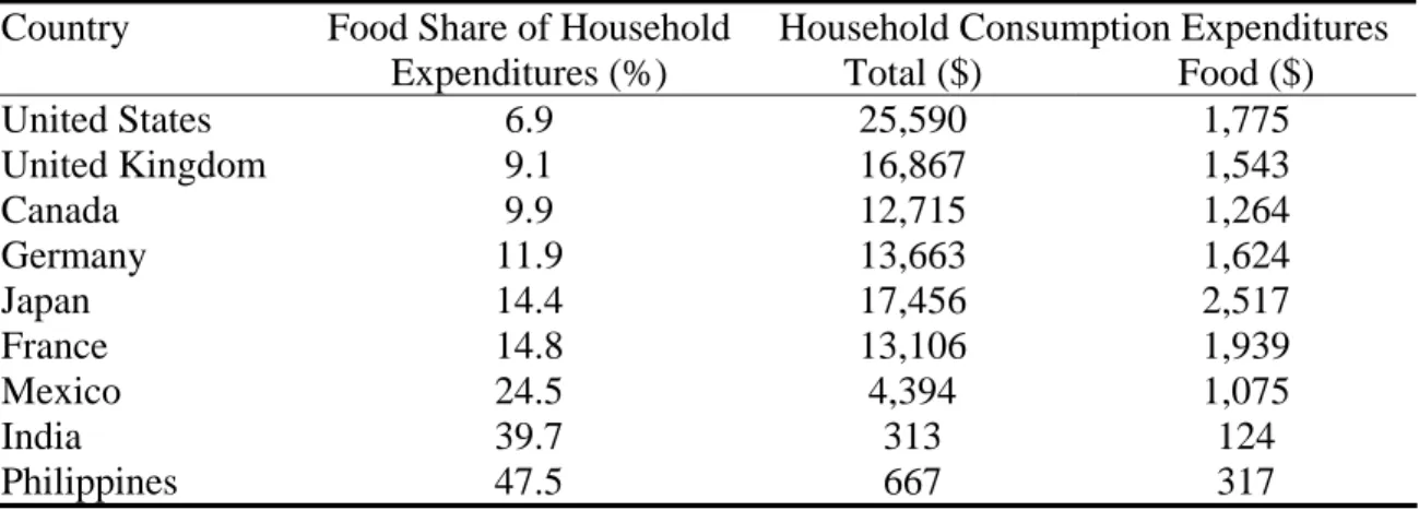
disposable personal income spent on food in the U.S. has steadily dropped to 9.5% in 2004 (USDA-ERS, 2006b). Over that period of time, real disposable personal income has experienced a 14.3 fold increase while the amount of money spent on food has increased only 4.7 times. When compared to other countries in terms of the amount of money spent on food as a percentage of all household expenditures, U.S. consumers easily spend the lowest amount (table 2). Although U.S. consumers spend a smaller share of all household expenditures on food, it must be noted that total household expenditures are significantly higher in the U.S. than the other countries listed in table 2.
Are farm subsidies responsible for the fact that U.S. consumers spend relatively less on food than other countries? A recent paper addresses that question. Miller and Coble evaluated the impact that U.S. farm subsidies had on the proportion of disposable income spent on food. The study concluded that from 1960-1999, government payments to farmers were not statistically significant in determining the percentage of disposable income spent of food. Rather, disposable income, productivity, and the farm-to-retail spread of food commodities had a statistically significant impact on the proportion of disposable income spent on food.
7
Pe rce ntage of Disposable Income Spe nt on Food in U.S.
0 5 10 15 20 25 30 1929 1939 1949 1959 1969 1979 1989 1999 P e rc en t
Away from home At home
Figure 4
Table 2. Share of Household Final Consumption Expenditures Spent on Food by Selected Countries, 2002.
Household Consumption Expenditures Country Food Share of Household
Expenditures (%) Total ($) Food ($) United States 6.9 25,590 1,775 United Kingdom 9.1 16,867 1,543 Canada 9.9 12,715 1,264 Germany 11.9 13,663 1,624 Japan 14.4 17,456 2,517 France 14.8 13,106 1,939 Mexico 24.5 4,394 1,075 India 39.7 313 124 Philippines 47.5 667 317 Source: USDA-ERS, 2005.
The argument that farm subsidies provide a cheap food supply to U.S. consumers does not withstand scrutiny. The argument is especially misplaced with commodities such as milk and sugar that are beneficiaries of price supports and supply controls that keep the prices U.S. consumers pay above world equilibrium prices. Such policies are especially burdensome on the poor, who spend a higher portion of their disposable income on food.
Maintain the Environment
Another popular justification for farm programs in general is that they help farmers maintain the environment. The argument made by farm program supporters is that in agricultural production, there are costs in terms of environmental degradation that are not covered by the market. Consequently, government policies are needed to compensate farmers for environmental practices that are not supported by the market. Environmental degradation in agricultural production can take place in two forms. The first type is environmental loss that occurs exclusively on the land being farmed. An example of this form of loss would be cropland that diminishes in productivity due to soil erosion. In
such a situation, the relevant question is, Do the costs of maintaining the soil outweigh the benefits to the farmer? If the costs are higher than the benefits, then the argument could be made that society may be well served by implementing policies that would encourage soil conservation practices (through subsidies, incentives, and/or regulations). However, even in this case, as long as land is transferable, there is a market incentive for the farmer to maintain the soil. If the market benefits from soil conservation outweigh the costs, then there are sufficient incentives for farmers to adopt conservation practices, without government intervention.
The second form of environmental loss is externalities that affect not the farmer, but others. Examples of externalities from agricultural production include soil sediments in rivers and other bodies of water, contamination of groundwater from chemicals and fertilizers, blowing dust, and odors from confined livestock operations. Unlike
environmental losses exclusive to the farmer, the market may not address these external costs. Once again, if that is the case, then society may benefit from government
intervention.
If government intervention is deemed appropriate for reducing externalities in agriculture, the next logical question is, What type of program(s) is best suited to accomplish that goal? Supporters of income support programs may argue that these programs would help provide market incentives for conservation practices. Certainly, income support programs may provide increased income, but they also result in higher costs in terms of land rents. Therefore, whether income support programs provide sufficient incentives for farmers to implement conservation practices is debatable.
There is little debate, however, that income support programs can result in some unintended environmental consequences. Notably, income supports such as marketing loans, counter-cyclical payments, and direct payments provide incentives for farmers to produce crops on environmentally sensitive (and likely less profitable) land that
otherwise may not be cropped. Likewise, these programs encourage the use of fertilizers and chemicals above market equilibrium levels. Excessive use of fertilizers and
chemicals can have significant negative environment consequences. Based on these consequences, it is questionable whether income support programs provide a net benefit to the agricultural environment.
Compete with Subsidizing Countries and Large Agribusinesses
A final justification offered for farm subsidies relates to the ability of U.S. farmers to compete with large domestic agribusinesses and subsidized foreign farmers. In terms of the domestic agribusiness justification, the basic argument is that given the market structure of general commodity production, farmers are pinched between a few large input suppliers and a few large commodity purchasers. In other words, large input suppliers have the advantage of market power on the cost side of farming while large grain and livestock processing companies have the advantage of market power on the revenue side of farming. Consequently, the “typical” farmer has little to no market power.
9
Another reason given for the need for farm subsidies is to compete with other countries that subsidize their producers. Ultimately these subsidies would reduce world prices, causing the prices U.S. farmers receive to drop as well. Subsidies are then needed in the U.S. to make up for the lower prices farmers are receiving. Another reason given for U.S. subsidies is that U.S. producers are priced out of foreign markets by export
subsidies, price support programs, and/or import restrictions enacted by other countries.
Agribusiness Competition
As previously mentioned, large agribusinesses are frequently accused of exercising market power to the detriment of small farmers. Given this accusation, two relevant questions come to mind. First, is there evidence that large agribusinesses routinely exercise market power at the expense of small farmers? Second, if market power is exercised, does it warrant subsidies to U.S. farmers.
A number of economic studies have been conducted over the last couple of decades to determine whether large agribusinesses systematically exert market power against U.S. farmers. A summary of these studies is discussed in Tweeten and Thompson (p. 128-138). The general conclusion that can be drawn from these studies is that agribusiness markets “are imperfectly competitive, but cost efficiencies resulting from greater concentration exceed losses from market power distortions” (p.142). More specifically, U.S. farmers are not hurt by the application of market power of agribusinesses, and consumers gain from lower costs brought forth from economies of scale. Actually, the concentration of agribusinesses on the input supply side of farming may benefit farmers through gains in research and development and production efficiencies that would not be possible if production were diffused among more numerous, smaller companies.
Likewise, farmers may also benefit from advertising campaigns used by large processing and retail agribusinesses that increase the demand for food. Therefore, the strongest conclusion that may be drawn from this discussion is that justifying farm programs on the basis of competition with large agribusinesses is, at best, a weak argument.
Foreign Subsidies and Trade Barriers
Trade between countries occurs when it is mutually beneficial to the buyer (importer) and seller (exporter). After instituting protectionist trade policies in the 1930s, U.S.
agricultural exports did not recover their share of farm marketings until the late 1970s (Pasour p. 160). In recent years, exports have been crucial to many agricultural commodities.
Compared to the high level of agricultural exports in the early 1980s, exports as a share of production have risen for some commodities and fallen for others. Whether exports as a share of production have risen or fallen over the last two decades, they are very
important for many commodities in the U.S. For example, nearly 47% of food grains and 57% of cotton/tobacco were exported in 2002 (USDA, 2003). Obviously, exports are critical to U.S. agriculture. So policies, both domestic and foreign, that are conducive to trade are generally beneficial to U.S. farmers. However, global trade is extremely complex as it is influenced by many factors outside the control of the interested
participants. These factors include macroeconomic issues such as exchange and interest rates, other trade policies, such as trade barriers on other products or commodities, and foreign policy actions. Because of the impact that these factors may have on U.S. farms, producers call for farm subsidies.
The relevant question then becomes: Do farm subsidies benefit U.S. farmers in light of other countries’ subsidies and protectionism? Because trade is complex, the answer to the posed question is complex. Certainly, farmers in the U.S. are affected by the farm and trade policies of other countries. A typical result of those actions is to lower the price that U.S. farmers receive for their goods—whether those actions are by subsidies or trade barriers. A typical response in the U.S. is to institute subsidies or trade barriers. That response has economic implications as well.
If the U.S. implements price supports or import restrictions, U.S. producers will likely experience higher prices. But those higher prices will have implications beyond what the producer will receive. First, higher U.S. prices cost U.S. consumers of those products—a fact that is often overlooked and contrary to the “cheap food supply” justification of farm subsidies. That additional cost will also reduce the quantity demanded by U.S.
consumers, putting downward pressure on U.S. domestic prices. Second, U.S. actions will affect our ability to export. To the extent that the U.S. institutes price support or pseudo price support (i.e. marketing loan) programs that ultimately result in increased production and reduced market prices, it can be expected that exporting countries
affected U.S. actions will respond with subsidies or protectionist measures of their own.
Although it may be known that subsidies or trade barriers may be harmful to the overall economy, it may not be politically expedient to stand by while a domestic industry suffers because of the actions of another country. This is why trade negotiations are so difficult. A recent report from the Organization for Economic Cooperation and
Development (OECD) estimated that $44 billion in welfare gains would be generated if subsidies and trade barriers throughout the world were halved. Another study by the International Food Policy Research Institute (IFPRI) estimates that there would be $200 billion in income gains in the global economy if trade was fully liberalized (Bouet, et al.). Those who had the highest support and protection would gain the most from the reforms. However, local political interests often outweigh larger economic benefits, (as evidenced by the recent suspended WTO trade negotiations) making reductions in subsidies and trade barriers difficult to achieve.
Summary
This paper discusses five of the most common economic justifications for farm subsidies. When analyzed in depth, those justifications are not always as valid as they may seem at first. Certainly, there are challenges facing U.S. farmers. Problems of variability of income are real to many farmers and rural communities. From the 1930s onward, the reaction of the U.S. government to these challenges has been to subsidize selected farm commodities. Those subsidies, however, often have unintended consequences that mitigate their intended purposes. Likewise, as time goes by, programs can become outdated and ineffective. So while the goal of farm subsidies may be noble, their actual
11
effect may be limited. Therefore, the question rising out of this discussion may not be, Should we eliminate farm subsidies? Rather, the question may be, Are there farm policy options that would better serve U.S. agriculture, taxpayers, and consumers?
Resources
Banker, D.E. and J.M. MacDonald, Eds. 2005 Structural and Financial Characteristics of U.S. Farms: 2004 Family Farm Report. Agriculture Information Bulletin No. 797. USDA-ERS.
Bouet, A., S. Mevel, and D. Orden. 2006. Two Opportunities to Deliver on the Doha Development Pledge. International Food Policy Research Institute. Research Brief No. 6, July 2006.
Browne, W.P., J.R. Skees, L.E. Swanson, P.B. Thompson, and L.J. Unnevehr. 1992.
Sacred Cows and Hot Potatoes: Agrarian Myths in Agricultural Policy. Westview Press.
Dimitri, C., A. Effland, and N. Conklin. 2005. The 20th Century Transformation of U.S. Agriculture and Farm Policy. Economic Information Bulletin No. 3. USDA-ERS.
Drabenstott, M. 2005. Do Farm Payments Promote Rural Economic Growth? Center for the Study of Rural America. Federal Reserve Bank of Kansas City.
Farm Foundation—National Public Policy Education Committee. 2006. The 2007 Farm Bill: U.S. Producer Preferences for Agricultural, Food, and Public Policy. Publication No. 2006-01.
Hoppe, R.A. and D.E. Banker. 2006. Structural and Finances of U.S. Farms: 2005 Family Farm Report. Economic Information Bulletin No. 12. USDA-ERS.
Jones, C.A., H. El-Osta, and R. Green. 2006. Economic Well-Being of Farm Households. Economic Brief No. 7. USDA-ERS.
Kastens, T. and K. Dhuyvetter. Government Program Payments and Non-agricultural Returns Affect Land Values.www.agmanager.info. September, 2006.
McGranahan, D.A. and C.L. Beale. 2002. Understanding Rural Population Loss. Rural America. Vol. 17, Issue 4. USDA-ERS.
Miller, J.C. and K.H. Coble. 2005. Cheap Food Policy: Fact or Rhetoric? Selected paper at AAEA Annual Meeting. Providence, RI. July, 2005.
OECD. 2006. Agricultural Policy and Trade Reform: Potential Effects at Global, National, and Household Levels. http://www.oecd.org.
Pasour, Jr., E.C. 1990. Agriculture and the State: Market Processes and Bureaucracy. The Independent Institute.
Tweeten, L. and S.R. Thompson, Eds. 2002. Agricultural Policy for the 21st Century. Iowa State Press.
USDA. 2006. Rural Development. 2007 Farm Bill Theme Papers.
USDA-ERS. 2003. Amber Waves. Indicators, p. 47. Nov. 2003.
USDA-ERS. 2005. Expenditures on Food, by Selected Countries, 2002. http://www.ers.usda.gov/Briefing/CPIFoodAndExpenditures/Data/table97.htm
USDA-ERS. 2006a. Farm Income and Balance Sheet Indicators, 1929-2006. http://www.ers.usda.gov/Briefing/FarmIncome/Data/Constant-dollar-table.XLS
USDA-ERS. 2006b. Food Expenditures by Families and Individuals as a Share of Personal Disposable Income.
http://www.ers.usda.gov/Briefing/CPIFoodAndExpenditures/Data/table7.htm
1
The 2007 Farm Bill: Status Quo With Adjustments
Bradley D. Lubben Extension Public Policy Specialist
University of Nebraska-Lincoln
Troy J. Dumler
Extension Agricultural Economist Kansas State University
In the policy world of options and consequences, one option is always to maintain the status quo. For federal farm programs, that implies re-authorizing or extending the basic three-part farm income safety net established in the 2002 Farm Bill.
Three-Part Safety Net Program
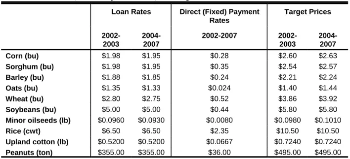
That safety net includes marketing assistance loans, direct payments, and counter-cyclical payments that work together in an integrated net to provide protection based on a target price level for the various program commodities. The original rates implemented in the 2002 Farm Bill are listed in Table 1.
Table 1. Loan Rates, Direct Payment Rates, and Target Prices for Covered Commodities Loan Rates Direct (Fixed) Payment
Rates Target Prices 2002-2003 2004-2007 2002-2007 2002-2003 2004-2007 Corn (bu) $1.98 $1.95 $0.28 $2.60 $2.63 Sorghum (bu) $1.98 $1.95 $0.35 $2.54 $2.57 Barley (bu) $1.88 $1.85 $0.24 $2.21 $2.24 Oats (bu) $1.35 $1.33 $0.024 $1.40 $1.44 Wheat (bu) $2.80 $2.75 $0.52 $3.86 $3.92 Soybeans (bu) $5.00 $5.00 $0.44 $5.80 $5.80 Minor oilseeds (lb) $0.0960 $0.0930 $0.0080 $0.0980 $0.1010 Rice (cwt) $6.50 $6.50 $2.35 $10.50 $10.50 Upland cotton (lb) $0.5200 $0.5200 $0.0667 $0.7240 $0.7240 Peanuts (ton) $355.00 $355.00 $36.00 $495.00 $495.00
The three-part safety net starts with the marketing assistance loan program, which provides income support based on the national average loan rates as listed in Table 1 for each program commodity. This support comes as loan proceeds in the amount of the loan rate for each unit of commodity pledged under the loan program. The loan program has changed over the years to become a marketing loan, meaning that the program allows for the loan to be repaid by the producer at a rate based on the market price. If market prices are below the loan rate, the loan can be repaid at the lower of the posted county price, which reflects the local market prices, or the loan rate plus interest. When the loan is repaid at a posted county price below the loan rate, the difference between the loan rate and the repayment rate is called a marketing loan gain (MLG) and represents a benefit to the producer. Alternatively, a producer can request a loan deficiency payment (LDP) in lieu of a loan. The LDP is equal to the same difference between the loan rate and the relevant posted county price. The marketing loan program benefits in the form of MLGs or LDPs are subject to a $75,000 per person payment limit or a $150,000 limit under the three-entity rule with current farm program rules, although other features of the marketing loan program allow for loan repayment with certificates or through forfeitures that effectively preclude the impact of these payment limits for most producers.
The direct payment is the second part of the current safety net. It first appeared in the 1996 Farm Bill and guarantees a fixed payment to producers based on the producer’s base acreage and program yield history multiplied by a fixed payment rate and then multiplied by 85 percent. The direct payment insures a
payment to producers regardless of production or market price and also allows producers almost unlimited flexibility to grow any crop, except for fruits and vegetables, on the direct payment acre. Direct payments are subject to a $40,000 per person payment limit, or $80,000 under the full effect of the three-entity rule. Counter-cyclical payments are the third part of the safety net established in the 2002 Farm Bill. They provide a payment based on the difference between the target price as listed in Table 1 and the effective market price for the commodity. That rate is then multiplied by the producer’s based acreage and program yield history multiplied by 85 percent. The effective market price is equal to the direct payment rate plus the higher of the marketing loan rate or the actual national average market price. Counter-cyclical
payments are subject to a $65,000 per person payment limit, or $135,000 under the full effect of the three-entity rule.
2007 Farm Bill Proposals
There have been several calls for maintaining the basic elements of the 2002 Farm Bill in the new legislation. In USDA’s farm bill proposals released in late January, the basic structure of the three-part safety net was retained, although the counter-cyclical payment would shift from a price-based payment to a revenue-based payment. USDA also proposed some adjustments in the basic rates of the marketing loan and direct payments as shown in Table 2.
Table 2. USDA Farm Bill Recommendations for Marketing Loan Rates and Direct Payments
Loan Rates Direct (Fixed) Payment Rates Current Average of Proposed Rates, 2008-2012 Proposed Maximum Current Proposed 2008-2009, 2013-17 Proposed 2010-2012 Corn (bu) $1.95 $1.89 $1.89 $0.28 $0.28 $0.30 Sorghum (bu) $1.95 $1.89 $1.89 $0.35 $0.35 $0.37 Barley (bu) $1.85 $1.70 $1.70 $0.24 $0.25 $0.26 Oats (bu) $1.33 $1.21 $1.21 $0.02 $0.02 $0.03 Wheat (bu) $2.75 $2.58 $2.58 $0.52 $0.52 $0.56 Soybeans (bu) $5.00 $4.92 $4.92 $0.44 $0.47 $0.50 Minor oilseeds (lb) $0.0930 $0.0870 $0.0870 $0.0080 $0.0080 $0.00857 Rice (cwt) $6.50 $6.50 $6.50 $2.35 $2.35 $2.52 Upland cotton (lb) $0.5200 $0.4570 $0.5192 $0.0667 $0.1108 $0.1108 Peanuts (ton) $355.00 $336.00 $336.00 $36.00 $36.00 $38.61
USDA specifically proposes to establish the marketing loan rates at 85 percent of the five-year Olympic average market price (eliminating the high and low years), subject to a maximum loan rate as established in the U.S. House of Representatives version of the 2002 Farm Bill. The change in maximum rates would mean lower loan rates for most commodities, particularly for upland cotton. USDA also proposes direct payments that are predominantly in keeping with the existing direct payment rates for the first two years of the new farm bill before increasing slightly over the last three years of a presumed five-year farm bill before reverting to the former rates at the end of the next farm bill.
3
calculation and the posted county price for purposes of the LDP would apply to the day beneficial interest is lost, removing the flexibility to establish the LDP or loan repayment rate separately from the time of cash marketing.
The marketing loan program and the direct payments as proposed by USDA represent only part of the proposed safety net. The third leg of USDA’s proposal shifts the counter-cyclical payment based on price to one based on revenue as discussed in the revenue safety net paper.
Several other groups have offered support for the existing safety net. The National Association of Wheat Growers and the American Soybean Association have both offered formal recommendations to retain the basic elements of the existing safety net. The wheat growers have argued for increases in direct payments and target prices and the soybean growers have proposed higher loan rates and target prices.
Five-Part Safety Net Issues
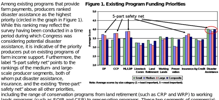
While the existing farm legislation focuses on the existing three-part safety net from the 2002 Farm Bill, the debate encompasses a much larger discussion of several programs that represent a mix of price, production, and revenue tools. On top of the three-part safety net, producers have also benefitted from insurance programs that have become more innovative and more attractive in terms of protection and premium subsidies. And, producers have often seen and expected disaster assistance in recent years, even though it is neither formally authorized nor budgeted. In a recent nationwide survey conducted at the University of Nebraska-Lincoln in conjunction with 26 other states, thousands of agricultural producers were queried on their policy preferences heading into the new farm bill (for more information on the survey, see the national report on the web at www.farmfoundation.org or at
www.agecon.unl.edu/pub/2007farmbill.pdf). In response to a question about existing program priorities, producers ranked several programs on a scale of 1 (least important) to 5 (most important). The results, broken down by the size group of the producer respondents, show this broad support for the basic farm income safety net (Figure 1).
Among existing programs that provide farm payments, producers ranked disaster assistance as the highest priority (circled in the graph in Figure 1). While this ranking may reflect the survey having been conducted in a time period during which Congress was considering potential disaster
assistance, it is indicative of the priority producers put on existing programs of farm income support. Furthermore, the label “5-part safety net” points to the rankings of the medium- and large-scale producer segments, both of whom put disaster assistance,
insurance, and the existing “three-part” safety net” above all other priorities,
including the range of conservation programs from land retirement (such as CRP and WRP) to working lands programs (such as EQIP and CSP) to preservation programs. These two segments of commercial-size agricultural producers clearly place the safety net as a high priority in the farm bill debate.
Related Issues
Beyond the basic structure of the commodity programs and the farm income safety net, there are some policy issues that will be addressed in any re-authorization of the status quo. Three issues likely to be
2.0 2.5 3.0 3.5 4.0 4.5 5.0 DP CCP ML/LDP Livestock Comm Land Retirement Working Lands Preser-vation
Insurance Ag Credit Disaster Assistance A ver ag e S c o re
Small Medium Large Composite
5-part safety net
Note: Average scores by size category (1 = least important, 5 = most important). 2.0 2.5 3.0 3.5 4.0 4.5 5.0 DP CCP ML/LDP Livestock Comm Land Retirement Working Lands Preser-vation
Insurance Ag Credit Disaster Assistance A ver ag e S c o re
Small Medium Large Composite
5-part safety net 5-part safety net
Note: Average scores by size category (1 = least important, 5 = most important).
discussed as potential adjustments to the status quo include payment limits, fruit and vegetable planting restrictions, and permanent authority for disaster assistance.
Payment limits have been a topic of debate for some time and are likely to again be part of the primary debate on the farm bill. Current payment limit rules set individual payment limits per person at $40,000 for DPs, $65,000 for CCPs, and $75,000 for ML/LDP benefits. In addition, a person can qualify for full payments in one entity, plus up to half the payments in a second and third entity. This three-entity rule means that the individual combined limit of $180,000 could equal up to $360,000 per person, if all individual categories are maximized. In addition, the marketing loan program includes language allowing repayment of commodity loans with certificates such that the loan gains would not count against the limit. All three of these issues - the individual payment limits, the three-entity rule, and the unlimited certificate loan gains - are likely to be debated.
Potential changes could lower the overall limits and reduce payments to some program participants, theoretically reducing program spending. USDA’s proposed farm bill recommendations would attribute payments directly to individuals, eliminate the three-entity rule, and make modifications to the overall payment limits for each part of the program. More significantly, USDA proposes a change in the program eligibility rules for adjusted gross income. The current eligibility rules state that to be eligible for farm programs, individuals must have an average adjusted gross income of $2.5 million or less or have at least 75 percent of the adjusted gross income from agricultural activities. The proposed rules would shift the cap to $200,000 and eliminate the 75-percent exclusion.
Alternatively, such changes may push producers to simply adjust their business structure to legally comply with any changed rules without leaving potential program payments unclaimed. Regardless of any
changes, this issue will likely continue to be a primary focal point for debate.
The fruit and vegetable planting restriction is also due to be addressed within the scope of existing
commodity programs and could particularly impact dry bean producers in Nebraska and other Great Plains regions. Under current program rules, producers cannot enroll in the DP and CCP program and also plant fruits and vegetables on the enrolled acreage. This planting restriction dates back several years. As producers were given more flexibility to make cropping decisions without giving up program payments, this restriction prevented them from shifting acres to fruit and vegetable production and directly competing with specialty crop growers who did not received direct crop support payments. The planting restriction became an issue in the WTO cotton case filed against the United States by Brazil. Since the planting restriction was interpreted to be affecting production decisions, the DPs, which were thought to be decoupled from production and thus, trade-legal, were found to not be fully decoupled and thus counted against U.S. spending limits.
In the aftermath of the WTO dispute, it has been widely expected that the restriction would be removed to eliminate the trade impact. However, that brings the fruit and vegetable industry to the table with major concerns over farm programs and spending. If the planting restriction disappears, the specialty crop sector has argued that they need part of the farm program spending pie. They have also argued that the value of fruit, vegetable, and other specialty crop production is fully half of the nation’s value of crop production in 2006 (USDA-ERS) and thus, are deserving of program support in the billions of dollars on par with program commodities, perhaps as much as 50 percent, or $4.7 billion of the estimated $9.4 billion in spending on direct and counter-cyclical payments to program crop producers in 2006 (USDA-ERS). Conversely, the potential economic impact on fruit and vegetable growers of eliminating the planting restriction might be estimated by the value of government payments a producer would have to give up to make the switch in production. Using the $9.4 billion estimate from 2006 spread over approximately 350 million crop acres enrolled in the federal farm program (USDA-FSA), the average government payment was approximately $27 per program base acre. If that amount were budgeted over the approximately 12 million acres nationwide of fruits, vegetables, dry beans, and potatoes (2002 Census of Agriculture), the
5
do with fruits and vegetables is far from decided. The simple calculations above potentially put boundaries on the debate, but the range of just over $300 million to more than $4 billion is hardly concise. USDA’s proposed farm bill recommendations include the elimination of the planting restriction and the proposed addition of more than $500 million per year for fruit, vegetable, and specialty crop programs on market development, food program purchases, and production research.
Finally, the role of agricultural disaster assistance, its regular implementation over the past several years, and its political support among producers have led to some calls to make it permanent. Currently, disaster assistance has been ad hoc authority developed by Congress to address production and/or economic losses in agriculture from year to year. In regularly passing some form of assistance on an ad hoc basis, Congress is often challenged to declare it emergency spending or to find funding by cutting spending in other areas. The two recent disaster assistance packages passed in 2003 for 2001 and 2002 losses and in 2004 for 2003 and 2004 losses both were funded in part by cutting spending projections for
conservation programs. This continual fight for funding is part of the reason any potential assistance for losses from the 2005 crop year is still unresolved. Making disaster assistance permanent would simply add the authority for the program to be carried out each year as needed. Of course, making it permanent would also add several billion in expected spending levels to the farm program at a time when budget, trade, and political constraints may not allow it.