Multilevel Approximate Robust Principal Component Analysis
Vahan Hovhannisyan
Yannis Panagakis
Stefanos Zafeiriou
Panos Parpas
Imperial College London, UK
{v.hovhannisyan13, i.panagakis, s.zafeiriou, p.parpas}@imperial.ac.uk
Abstract
Robust principal component analysis (RPCA) is cur-rently the method of choice for recovering a low-rank ma-trix from sparse corruptions that are of unknown value and support by decomposing the observation matrix into low-rank and sparse matrices. RPCA has many applications including background subtraction, learning of robust sub-spaces from visual data, etc. Nevertheless, the application of SVD in each iteration of optimisation methods renders the application of RPCA challenging in cases when data is large. In this paper, we propose the first, to the best of our knowledge, multilevel approach for solving convex and non-convex RPCA models. The basic idea is to construct lower dimensional models and perform SVD on them in-stead of the original high dimensional problem. We show that the proposed approach gives a good approximate solu-tion to the original problem for both convex and non-convex formulations, while being many times faster than original RPCA methods in several real world datasets.
1. Introduction
Low-rank matrix recovery is a cornerstone in data analy-sis and dimensionality reduction, with the principal compo-nent analysis (PCA) [12] being the most widely employed method for this task. Even though the PCA is easy to do by means of eigen-decomposition, it is fragile to the prence of gross, non-Gaussian noise and outliers and the es-timated low-rank subspace may be arbitrarily away from the true one; even when a small fraction of the data is cor-rupted [14]. To alleviate this, robust PCA (RPCA) models have been proposed [6]. The RPCA aims to recover a low-rank matrix from sparse corruptions that are of unknown value and support by decomposing the observation matrix (D) into two terms: a low-rank matrix (L) and a sparse
one (S) , accounting for sparse noise and outliers, namely D=L+S. This model has profound impact in visual data
analysis and computer vision applications such as image de-noising [6], background substraction, image alignment [25],
texture recovery [30], deformable models [26], face frontal-ization [27], structure from motion [2], to mention but a few examples.
A natural approach to estimate the low-rank plus sparse decomposition of the RPCA is to minimize the rank ofL
and the number on non-zero entries of S , measured by ℓ0quasi norm [6]. Unfortunately, both rank andℓ0-norm minimization is NP-hard [29,21]. The nuclear- and theℓ1 -norms are typically adopted as convex surrogates to rank and ℓ0- norm, respectively yielding a convex relaxation, which can be provably solved under some natural condi-tions on the low rank and sparse components. Common solvers for the convex RPCA include: Iterative Threshold-ing (IT) [8], Accelerated Proximal Gradient (APG) [24], Augmented Lagrange Multipliers (ALM) and Augmented Lagrangian Alternating Direction method [16]. However, the above mentioned solvers exhibit significant computa-tional drawbacks. In particular, the convex RPCA model can be solved with at mostO(1/ǫ)iterations, whereǫis the solution accuracy, each iteration requires a singular value decomposition (SVD), which can be computationally ex-pensive even when only a few singular values are calculated. Moreover, theO(1/ǫ)convergence rate is much slower that theO(log(1/ǫ))rate of the classical PCA.
Recent advances in non-convex optimization enable the development of algorithms that partially alleviate the com-putational burden of convex RPCA. Concretely, Netrapalli et al [22] proposed to solve a non-convex problem of finding a low rank plus sparse matrix decomposition, by means of alternating projections onto non-convex sets. Surprisingly, the method provably converges to a unique minimiser with linear rateO(log(1/ǫ)), which is much faster that the sub-linear rate of convex methods. However, for large problems (even partial SVDs) can require unacceptably long time to solve the problem. There have been several attempts to re-duce the computational time of large nuclear norm regu-larized optimization problems. Namely, [17] proposed to reduce the problem dimension by writing the large solution matrix as a product of a small orthogonal and another ma-trix. They solved the resulting non-convex problem via an
augmented Lagrangian alternating direction method. An-other very popular approach for reducing large problem di-mensions is to create smaller sub-problems using various randomized techniques [18,23,9,19,1].
In this paper, motivated by the recent advances in mul-tilevel optimization algorithms [20,13] we propose a sim-ple, yet quite generic and very effective approach for signif-icantly reducing computational costs for many problems re-quiring low rank matrix approximations, including convex and non-convex robust PCA models. We exploit the fact that many problems arising from computer vision and ma-chine learning applications can be modelled using various degrees of fidelity. For instance, video frames from a fixed camera or facial images taken with varying illuminations are highly correlated and therefore their linear combina-tions maintain the model’s underlying information. The ba-sic idea is to construct and solve lower dimensional (coarse) models for each subproblem and then prolong its solution to the original problem dimension. We show that using special restriction and prolongation operators ensure good low rank approximations. Then we demonstrate our proposed multi-level low rank approximation technique within both convex and non-convex models. As several video background ex-traction and facial shadow removal experiments show, our multilevel approach can speed up its original method by several times.
Notations.Throughout the paper, scalars are denoted by case letters, vectors (matrices) are denoted by lower-case (upper-lower-case) boldface letters, e.g. x(X). Idenotes
the identity matrix with appropriate dimension. Theℓ1and
ℓ2 norms of a vectorxare defined askxk1 =Pi|xi|and
kxk2 =pP
ix2i, respectively. The matrixℓ1norm is
de-fined askXk1 = P
i
P
j|xij|, where| · |denotes the
ab-solute value operator. The Frobenius norm is defined as
kXkF = qP
i
P
jx2ij, and the nuclear norm ofX (i.e.,
the sum of singular values of a matrix) is denoted bykXk∗.
Thel-th largest (in absolute value) singular value of matrix
Xis denoted asσl(X). In algorithm pseudocodes we use X(k)(uk) to denote the value of matrixX(scalaru) at iter-ationk.
2. RPCA Methods
In this section, we present the state of the art methods for solving the convex and non-convex robust PCA problems. Note that for both methods, the computational bottleneck are the SVDs requiringO(rmn)operations each, wherer
is the number of required singular values.
2.1. Inexact ALM for RPCA
The problem of representing an input data matrixD ∈
Rm×nas a sum of a low rank matrixL⋆and a sparse matrix S⋆can be exactly solved via the following convex
optimiza-tion problem: min
L,Sk
Lk∗+λkSk1, subject to D=L+S, (1)
whereλ >0is a weighting parameter. A classical approach for solving (1) is by minimizing its augmented Lagrangian defined as L(L,S,Y, µ) =kLk∗+λkSk1 +hY,D−L−Si +µ 2kD−L−Sk 2 F, (2)
whereY ∈ Rm×n is the Lagrangian variable andµ > 0
is a penalty parameter. (2) can be solved via alternating directions method, aka solve the problem for each variable separately at each iteration [16]. In this case each resulting subproblem has a closed form solution so that the algorithm iterates as follows:
1. Solve (2) forSwith fixedLandY. This is done by
element-wise soft thresholding the appropriate inter-mediate matrix, i.e. S(k+1) = S
λµ−1[D−L(k)+
µ−1Y(k)], where S
τ[M] is the soft thresholding
op-erator defined element-wise [8]:
Sτ[x] = (|x| −τ)+sgn(x). (3) 2. Solve (2) for L with fixed Sand Y or equivalently
solve min L {k Lk∗+µ 2kM−Lk 2 F}, (4)
whereM = D−Sk+µ−1Y(k). This in turn, can be done in closed form using the singular value thresh-olding operatorDτ[M][5], i.e. L(k+1) =Dµ−1[D− S(k+1)+µ−1Y(k)], where
Dτ[M] =USτ[Σ]V⊤, (5)
whereM=UΣV⊤is the SVD ofM.
3. Update Lagrange variablesYand penalty coefficients µ.
This procedure was dubbed Inexact ALM (IALM) in [16] and is formally given here in Algorithm1. Note that for practical efficiency only a few singular values are computed as suggested in [16].
2.2. Non-convex RPCA
In a recent paper Netrapalli et al proposed a new method for recovering a low-rank matrix from sparse corruptions [22]. Its main idea is to perform alternating projects onto low rank and sparse matrix spaces. Although these sets are not convex, projections onto them can be done efficiently
Algorithm 1Inexact ALM (IALM) Input: D∈Rm×n
1: fork←1to...do
2: // Solvearg min
S L(L(k+1),S,Y(k), µk) 3: S(k+1)← S λµ−1 k [ D−L(k+1)+µ−1 k Y (k)]
4: // Solvearg min
L L(L,S(k+1),Y(k), µk) 5: M←D−S(k+1)+µ−1 k Y (k) 6: (U,Σ,V)←SVD(M) 7: L(k+1)←US µ−1k [Σ]V ⊤
8: // Update the Lagrangian variable
9: Y(k+1)←Y(k)+µk(D−L(k+1)−S(k+1))
10: Updateµk←µk+1
11: end forreturn(L(k+1),S(k+1))
using the hard thresholding operator Hζ[x], which is
ap-plied on vectors and matrices element-wise, i.e.Hζ[X]i,j= Xi,j if|Xi,j| ≥ζ and0otherwise. Specifically, solve the
following non-convex problem of finding a low rank plus sparse matrix decomposition:
min
L k
D−Lk0, subject to rank(L)≤r, (6)
wherer is a given upper bound on the rank of low rank componentL⋆. Although the problem in (6) is not convex,
it can provably be solved in linear time under mild condi-tions. The main steps of the method are given in Algorithm
2, which alternatively solves two sub-problems at each iter-ation by fixing one variable and solving for the other. The main difference here is that the arising sub-problems are constrained with the corresponding non-convex sets, there-fore hard thresholding is used instead of soft thesholding.
Here SVD(M, l)returns the firstl singular values with
corresponding singular vectors. Although Algorithm2 re-quires only l singular values at stage l = 1, . . . , r, SVD operations are still the computational bottleneck.
3. Multilevel Approximate SVD
In this section, we present a simple and yet efficient method for calculating SVD of a matrixM ∈ Rm×n
in-spired from multilevel optimization algorithms [20, 13]. The main idea is to first create a lower dimensional coarse matrix and then calculate its SVD, which is then used for low rank approximations.
As in multilevel optimisation algorithms our method too uses so-called ”restriction” operators to construct coarse models. We denote the restriction operator asR and
as-sume that it has linearly independent columns.
Algorithm 2Alternating Projections (AltProj) Input: D∈Rm×n, target rankr
1: InitializeL(0)=0andS(0)=Hζ0(D−L(0)) 2: forStagel←1tordo
3: forIterationk←0toT do
4: // Solve arg min
L:rank(L)≤l kD−L−S(k)k2 2 5: M←D−S(k) 6: (U,Σ,V)←SVD(M, l) 7: L(k+1)←UHl[Σ]V⊤ 8: // Solvearg min
S:kSk0≤ζ kD−L(k+1)−Sk2 2 9: Update thresholdζas in [22] 10: S(k+1)← Hζ[D−L(k+1)] 11: ifσl+1(L(k+1))< ǫthen 12: return(L(T),S(T)) 13: else 14: S(0)←S(T) 15: end if 16: end for 17: end for 18: return(L(T),S(T)) Specifically, forR∈Rn×n 2 we use Rn=1 4 α 0 0 . . . 0 0 4−2α 0 0 . . . 0 0 α α 0 . . . 0 0 0 4−2α 0 . . . 0 0 0 α α . . . 0 0 . . . 0 0 0 . . . α α 0 0 0 . . . 0 4−2α 0 0 0 . . . 0 α (7)
for some0≤α≤1acting as a smoothing parameter. For instance, whenα= 1,Rnis the standard interpolation
op-erator [4], and whenα= 0,Rnsimply selects every other
column ofM.
Often in practice we use more than 2 levels of coarse models. Specifically, we use a restriction operator R = RnRn 2 . . . Rn H ∈R m×nH, whereRk∈Rk×k 2 is given as
in (7). For all experiments we used up to the deepest possi-ble levels, so thatnH > r, whereris the number of singular
values required by the overlying algorithm. Clearly,Rhas
linearly independent columns and thus is full rank, more-over, without loss of generality we can assume thatRhas
normalized columns so thatkRk2≤1.
Next, we use the restriction operatorR to present our
proposed CoarseSVD method for efficiently calculating ap-proximate SVDs in Algorithm3. The basic idea here is to first apply the restriction operator onMand then perform
Algorithm 3CoarseSVD Input: M∈Rm×n,R∈Rn×nH
1: MH←MR
2: (UH,ΣH,VH)←SVD(MH) 3: return(UH,ΣH,VH)
Then after finding a low rank approximation forM, we
”lift” it to the original fine problem dimension. As in mul-tilevel literature, this is done using the transpose of the re-striction operator. Proposition1characterizes the approxi-mate SVD after prolongation.
Proposition 1. The prolongationVH = V
HR⊤ of right
singular vectors satisfies 1. VH⊤VH=RRT
2. kVHVH⊤k=kR⊤Rk 3. kUHΣHV⊤
HR
⊤−Mk ≤δkMk,
for a constantδ >0and eitherk · k2andk · kF norms.
Proof. The first two results follow directly from the or-thogonality of VH. The third one is due to the fact that kM(RR⊤−I)k ≤δkMk, for
δ:=kRR⊤−Ik ≤1. (8)
4. Multilevel Algorithms via Coarse SVD
While both Inexact ALM and Alternating Projections algorithms are guaranteed to converge to the global op-tima with strong convergence rates, in practice performing SVDs still remains a computational bottleneck, especially for larger problems. To overcome this major obstacle we propose to instead construct lower dimensional counterparts for the computationally expensive parts of each algorithm and use their solutions for finding approximate solutions for the original fine level problems. In other words, we use the multilevel low rank approximation technique to accelerate both convex and non-convex robust PCA algorithms.4.1. Multilevel Inexact ALM
We begin this subsection by introducing the multilevel singular value thresholding (ML-SVT) operator defined as
DHτ[M] =UHSτ[ΣH]V⊤HR⊤, (9)
whereMR=UHΣHV⊤
His the SVD of the coarse model MH =MR. Note that the ML-SVT operator (9) requires
a SVD on am×nHmatrix - significantly cheaper than the m×nfor (5). The next theorem shows that the proposed ML-SVT operator gives a good approximate solution for problem (4).
Theorem 1. Assuming thatkRk2 ≤1and0< τ ≤σH,1, the ML-SVT operatorDH
τ [M]gives a
σH,1
τ2 (σ1+σH,1−τ
)-approximate solution to the problem (4), whereσH,1is the largest singular value ofMR.
Proof. The proof follows the steps of the proof of Theorem 2.1 of [5] and is given in the Appendix.
Then we can use the proposed ML-SVT operator to solve the corresponding subproblems of Algorithm (1) resulting the Multilevel Inexact ALM (ML-IALM) method given be-low as Algorithm4.
Algorithm 4Multilevel Inexact ALM (ML-IALM) Input: D,S(0),YH,(0) ∈Rm×n;µ0 1: fork←1to...do 2: S(k+1)← Sλµ−1 k [ D−LH(k+1)+µ−1 k Y(k)]
3: // Approx solvearg min
L L(L,S(k+1),Y(k), µk) 4: MH←(D−S(k+1)+µ−k1Y (k))R 5: (UH,ΣH,VH)←SVD(MH) 6: LH ←UHSµ−1[Σ H]V⊤H 7: LH(k+1)←L HR⊤ 8: // Continue as in Algorithm1 9: Y(k+1)←Y(k)+µk(D−LH(k+1)−S(k+1)) 10: Updateµk ←µk+1 11: end for
We finish this subsection with a remark that the same approach can be used to extend the Inexact ALM method for the more general matrix completion problem (Algorithm 6 in [16]). In this case the only difference is that instead of soft-thresholding, projection onto a simple convex spaceΩ is used to updateS(k+1), whereas updates forL(k+1)are the same and therefore multilevel SVD can be used.
4.2. Multilevel Alternating Projections
We apply the multilevel low rank approximation method of Algorithm3also within the non-convex alternating pro-jections algorithm. In this case we create coarse models for subproblems of finding low rank approximations for inter-mediate matricesM=D−S(k), solve these subproblems and lift their solutions to the original fine dimension.
Each iteration of the Alternating Projections algorithm requires solving
min
L∈Rm×nk
D−L−Sk2 s.t. rank(L)≤l, (10)
which has a closed form solution given by the hard thresh-olding operator as follows
ˆ
where Hl[x] is the hard thresholding operator and is
de-fined element-wise for vectors and matrices. Therefore, for this setting we use the hard thresholding operator on the coarse model to construct an approximate solution for prob-lem (10) as follows:
LH =UHHl[ΣH]V⊤
HR
⊤,
(12) whereMR=MH =UHΣHV⊤ is a SVD of the coarse
model. Notice that the multilevel operator computes SVDs on much smaller problems than the original algorithm in this case as well. Then in Theorem2we show that theLH
defined in (12) gives a good approximate solution for prob-lem (10).
Theorem 2. The multilevel low rank approximation proce-dure of (12) gives a(σ1+σH,1)-approximate solution of the problem (10), whereσH,1 is the largest singular value ofMH=MR.
Proof. The proof follows the proof of Eckhard-Young-Mirsky theorem [11] and is given in the Appendix.
Then we can use (12) inside Algorithm2 to efficiently solve the corresponding subproblem. The resulting method is presented in Algorithm5.
Algorithm 5 Multilevel Alternating Projections (ML-AltProj)
Input: D∈Rm×n, target rankr 1: InitializeLH(0)=0andS(0)=H
ζ0(D−L
H(0))
2: forStagel←1tordo
3: forIterationk←0toTdo
4: // Approx solve arg min
L:rank(L)≤l kD−L−S(k)k 2 5: MH←(D−S(k))R 6: (UH,ΣH,VH)←SVD(MH, l) 7: LH←UHHl[ΣH]V⊤ H 8: LH(k+1)←L HR⊤ 9: // Continue as in Algorithm2 10: Update thresholdζas in[22] 11: S(k+1)← H ζ[D−LH (k+1) ] 12: ifσl+1(LH (k+1) )< ǫthen 13: return(LH(T),S(T)) 14: else 15: S(0)←S(T) 16: end if 17: end for 18: end for 19: return(LH(T),S(T))
5. Experiments
To test the practical efficiency of the proposed methods we compare them with the standard Inexact ALM [16]and Alternating Projections [22] algorithms on several real life video background extraction and facial shadow removal problems. For the standard Inexact ALM and Alternat-ing Projections algorithms we used the provided Matlab code. Then for each multilevel variant we replaced the standard low rank approximation parts of respective algo-rithms with corresponding multilevel low rank approxima-tion code, keeping the rest of the algorithms unchanged. Particularly, we used the same optimality criteria, so that the comparisons are fair. All methods were tested in Matlab R2015a on a standard desktop machine with Intel Core i7 processor and 32GB RAM.
5.1. Video Background Extraction
First, we test the algorithms on real surveillance videos. Assume we are given a surveillance video from a fixed cam-era and the task is to separate the constant background from moving objects. This problem can be modeled as (convex or non-convex) RPCA [3]. We first stack each frame of the video as a column vector creating a data matrixD. Then,
since the fixed background remains (approximately) con-stant in each frame and the moving objects take a relatively small portion of each frame, they can respectively represent the low rank and sparse components of the RPCA decom-position. We tested all algorithms on 4 surveillance videos described below:
• highway:48×64×400; run2seconds
• copy machine:48×72×3400; run50seconds
• walk:240×320×794; run50seconds [28]
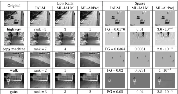
• gates:240×320×1895; run200seconds [28] The results are reported in Figure1. Each row represents a tested video. The first column contains sample frames from each corresponding video, then each of the following column triplets contains corresponding low rank and sparse components as returned from IALM and ML-IALM and ML-AltProj algorithms. We run IALM and ML-IALM for the same fixed time and ML-IALM until convergence with 10−7 error for reference. Below each frame we also re-port the corresponding achieved rank and the feasibility gap (FG) i.e.kD−L⋆−S⋆kF/kDkF. As the results indicate,
all algorithms produce similar results for all videos, except copymachine, for which ML-IALM produces significantly clearer separation of background than IALM. This is be-causecopy machinehas largest number of frames relative to the frame dimension.
We do not present frame samples from AltProj since it returns visually similar values to ML-AltProj. In this case,
Original Low Rank Sparse
IALM ML-IALM ML-AltProj IALM ML-IALM ML-AltProj
highway rank =5 3 1 FG =0.0176 0.01 3.6·10−4
copy machine rank =7 4 1 FG =0.0364 0.0031 2.8·10−4
walk rank =2 1 1 FG =0.02 0.0231 4·10−4
gates rank =3 3 2 FG =0.05 0.04 2.8·10−4
Figure 1: Examples from solving video background extraction problems via IALM, ML-IALM and ML-AltProj methods. IALM and ML-IALM run for a fixed CPU seconds, while ML-AltProj is given for reference and runs until convergence error 10−7. Each row corresponds respectively to highway(48×64×400), copy machine (48×72×3,400), walk (240×320×794) andgates(240×320×1,895) videos from top to bottom. With each frame we also report the respective rank of the low rank component and the feasibility gap (FG):kD−L−SkF/kDkF.
Problem AltProj ML-AltProj
highway 7 3 (2 levels) copy machine 54 12 (8 levels)
walk 467 261 (6 levels)
gates 744 354 (8 levels)
Table 1: CPU times (in seconds) after solving video back-ground removal problems up to tolerance 10−7 using the standard non-convex alternating projections algorithm and its multilevel variant.
we ran each algorithm until the same optimality error and report CPU times (in seconds) in Table 1. In all experi-ments we used up to 4-7 levels of coarse models (more for larger problems). In this case as well, the multilevel vari-ant largely outperforms the original algorithm. In fact, the larger the original problem, the bigger relative speed up can be achieved using the multilevel approach, since for larger
nwe can use deeper levels.
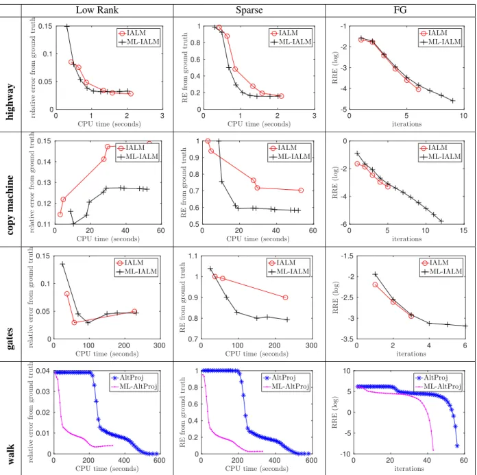
For further investigation of the convergence properties of IALM and AltProj algorithms compared to their multi-level variants, we measure the relative error of the current iterates compared to the ground truth(L0,S0)and FGs
dur-ing the iterations of both standard and multilevel algorithms through the same time interval. We report those relative
er-rors against CPU time (seconds) and iteration numbers in Figure2.
The plots suggest that ML-IALM performs only slightly faster than IALM on the smaller highwayexample, how-ever, as expected it is significantly faster on the largercopy machineandgatesproblems. As we could anticipate from the theory, at each iteration ML-IALM achieves a very good approximation as measured by the reconstruction er-ror, and since its iterations are significantly cheaper, it per-forms more iterations during the same time interval than IALM. We also report the results of running AltProj and ML-AltProj methods on thewalkproblem. The results are very similar to those observed in the convex model. ML-AltProj decreases the relative errors much earlier during the iterations and has significantly cheaper per iteration com-plexity.
5.2. Shadow Removal from Facial Images
Here we have a set of facial images from one or more individuals under various illuminations and the task is to re-move shadow/light noises from images. We used images of individuals from the Yale B facial extended database [10]. It contains (96×84) facial images of39subjects taken un-der various poses and illuminations each, with total2,414 images.
Low Rank Sparse FG
highway
CPU time (seconds)
0 1 2 3 re la ti v e er ro r fr o m g ro u n d tr u th 0 0.05 0.1 0.15 IALM ML-IALM
CPU time (seconds)
0 1 2 3 R E fr o m g ro u n d tr u th 0 0.2 0.4 0.6 0.8 1 IALM ML-IALM iterations 0 5 10 R R E (l o g ) -5 -4 -3 -2 -1 IALM ML-IALM copy machine
CPU time (seconds)
0 20 40 60 re la ti v e er ro r fr o m g ro u n d tr u th 0.11 0.12 0.13 0.14 0.15 IALM ML-IALM
CPU time (seconds)
0 20 40 60 R E fr o m g ro u n d tr u th 0.5 0.6 0.7 0.8 0.9 1 IALM ML-IALM iterations 0 5 10 15 R R E (l o g ) -6 -4 -2 0 IALM ML-IALM gates
CPU time (seconds)
0 100 200 300 re la ti v e er ro r fr o m g ro u n d tr u th 0 0.05 0.1 0.15 IALM ML-IALM
CPU time (seconds)
0 100 200 300 R E fr o m g ro u n d tr u th 0.7 0.8 0.9 1 1.1 IALM ML-IALM iterations 0 2 4 6 R R E (l o g ) -3.5 -3 -2.5 -2 -1.5 IALM ML-IALM walk
CPU time (seconds)
0 200 400 600 re la ti v e er ro r fr o m g ro u n d tr u th 0 0.01 0.02 0.03 0.04 AltProj ML-AltProj
CPU time (seconds)
0 200 400 600 R E fr o m g ro u n d tr u th 0 0.2 0.4 0.6 0.8 1 AltProj ML-AltProj iterations 0 20 40 60 R R E (l o g ) -10 -5 0 5 10 AltProj ML-AltProj
Figure 2: Comparing the relative errors during IALM, ML-IALM, AltProj and ML-AltProj iterations. The first two columns give relative errors compared to the ground truth (L0,S0), and the third column gives FGs during iterations. Each row
corresponds respectively tohighway(48×64×400),copy machine(48×72×3,400),walk(240×320×794) andgates (240×320×1,895) videos from top to bottom.
For this setting as well we test the multilevel SVD plugged into both IALM and AltProj methods. We ran both IALM and ML-IALM algorithms for5second and compare the returned results. While AltProj and ML-AltProj run un-til convergence with 10−7 error. The results are reported in Figure 3. Here as well each row represents a particu-lar database (individual). The first column contains sam-ple frames from each corresponding facial database, then
each of the following four columns contains correspond-ingly low rank and sparse components as returned from Inexact IALM, ML-IALM, AltProj and ML-AltProj algo-rithms. With each image we also report the corresponding achieved rank of the low rank component and the FG.
In order to compare the multilevel approach for the non-convex problem, we report the results after running AltProj and ML-AltProj algorithms until achieving convergence
er-Original Low Rank Sparse
IALM ML-IALM AltProj ML-AltProj IALM ML-IALM AltProj ML-AltProj
Yale B01 rank =5 10 10 10 FG =0.24 0.05 4·10−4 10−4
Yale B02 rank =5 10 10 10 FG =0.24 0.05 4·10−4 10−4
Yale B10 rank =3 10 10 10 FG =0.24 0.05 4·10−4 10−4
Figure 3: Examples from solving facial shadow removal problems via IALM, ML-IALM, AltProj and ML-AltProj algorithms on croppedYale Bdatabase (96×84×2414). We run both IALM and ML-IALM for fixed five seconds, while AltProj and ML-AltProj run until convergence with 10−7 error. With each image we also report the respective rank of the low rank component and the feasibility gap (FG):kD−L−SkF/kDkF.
Problem AltProj Ml-AltProj Yale B01 38.8 15.3 Yale B02 39.1 15.2 Yale B10 37.4 16.8
Table 2: CPU times (in seconds) after solving shadow re-moval problems up to a fixed tolerance using the standard non-convex alternating projections algorithm and its multi-level variant. For all experiments we used 2 multi-levels for the multilevel algorithm.
ror10−7 and record CPU times (seconds). The results are reported in Table 2. In all experiments we used up to3 levels of coarse models. In all experiments the multilevel algorithm is more than twice faster than its standard coun-terpart.
6. Discussion
In this paper we presented an approximate multilevel di-mension reduction method for efficient SVD calculations. We showed that the multilevel algorithms are theoretically good approximations to the original problem, and more-over, in practice they are significantly faster as demon-strated within convex and non-convex RPCA models. Fi-nally, its applications can be extended further to other SVD based methods, such as RASL [25] and matrix comple-tion [7]. More interesting applicacomple-tion of multilevel methods would be their application to tensor decomposition prob-lems (see [15] and references therein).
References
[1] Z. Allen-Zhu and Y. Li. Even faster svd decomposition yet without agonizing pain. InAdvances in Neural Information Processing Systems, pages 974–982, 2016.2
[2] R. Angst, C. Zach, and M. Pollefeys. The generalized trace-norm and its application to structure-from-motion problems. In2011 International Conference on Computer Vision, pages 2502–2509. IEEE, 2011.1
[3] T. Bouwmans, A. Sobral, S. Javed, S. K. Jung, and E.-H. Zahzah. Decomposition into low-rank plus additive matri-ces for background/foreground separation: A review for a comparative evaluation with a large-scale dataset.Computer Science Review, 2016.5
[4] W. L. Briggs, S. F. McCormick, et al. A multigrid tutorial. Siam, 2000.3
[5] J.-F. Cai, E. J. Cand`es, and Z. Shen. A singular value thresh-olding algorithm for matrix completion. SIAM Journal on Optimization, 20(4):1956–1982, 2010.2,4
[6] E. J. Cand`es, X. Li, Y. Ma, and J. Wright. Robust principal component analysis? Journal of the ACM (JACM), 58(3):11, 2011.1
[7] E. J. Cand`es and B. Recht. Exact matrix completion via con-vex optimization.Foundations of Computational mathemat-ics, 9(6):717–772, 2009.8
[8] I. Daubechies, M. Defrise, and C. De Mol. An iterative thresholding algorithm for linear inverse problems with a sparsity constraint. Communications on pure and applied mathematics, 57(11):1413–1457, 2004.1,2
[9] P. Drineas, R. Kannan, and M. W. Mahoney. Fast monte carlo algorithms for matrices ii: Computing a low-rank approxi-mation to a matrix.SIAM Journal on computing, 36(1):158– 183, 2006.2
[10] A. Georghiades, P. Belhumeur, and D. Kriegman. From few to many: Illumination cone models for face recognition un-der variable lighting and pose. IEEE Trans. Pattern Anal. Mach. Intelligence, 23(6):643–660, 2001.6
[11] G. H. Golub and C. F. Van Loan. Matrix computations, vol-ume 3. JHU Press, 2012.5
[12] H. Hotelling. Analysis of a complex of statistical variables into principal components. Journal of educational psychol-ogy, 24(6):417, 1933.1
[13] V. Hovhannisyan, P. Parpas, and S. Zafeiriou. Magma: Multilevel accelerated gradient mirror descent algorithm for large-scale convex composite minimization. SIAM Journal on Imaging Sciences, 9(4):1829–1857, 2016.2,3
[14] P. J. Huber.Robust statistics. Springer, 2011.1
[15] J. Kossaifi, Y. Panagakis, and M. Pantic. Tensorly: Tensor learning in python. InNIPS Tensor-Learn Workshop, 2016.
8
[16] Z. Lin, M. Chen, and Y. Ma. The augmented lagrange mul-tiplier method for exact recovery of corrupted low-rank ma-trices.arXiv preprint arXiv:1009.5055, 2010.1,2,4,5
[17] G. Liu and S. Yan. Active subspace: Toward scalable low-rank learning. Neural computation, 24(12):3371–3394, 2012.1
[18] R. Liu, Z. Lin, Z. Su, and J. Gao. Linear time principal com-ponent pursuit and its extensions using l1 filtering. Neuro-computing, 142:529–541, 2014.2
[19] C. Musco and C. Musco. Randomized block krylov meth-ods for stronger and faster approximate singular value de-composition. InAdvances in Neural Information Processing Systems, pages 1396–1404, 2015.2
[20] S. Nash. A multigrid approach to discretized optimization problems. Optimization Methods and Software, 14(1-2):99– 116, 2000.2,3
[21] B. K. Natarajan. Sparse approximate solutions to linear sys-tems.SIAM journal on computing, 24(2):227–234, 1995.1
[22] P. Netrapalli, U. Niranjan, S. Sanghavi, A. Anandkumar, and P. Jain. Non-convex robust pca. InAdvances in Neural In-formation Processing Systems, pages 1107–1115, 2014. 1,
2,3,5
[23] T.-H. Oh, Y. Matsushita, Y.-W. Tai, and I. So Kweon. Fast randomized singular value thresholding for nuclear norm minimization. In Proceedings of the IEEE Conference on Computer Vision and Pattern Recognition, pages 4484– 4493, 2015.2
[24] N. Parikh and S. Boyd. Proximal algorithms. Foundations and Trends in optimization, 1(3):123–231, 2013.1
[25] Y. Peng, A. Ganesh, J. Wright, W. Xu, and Y. Ma. RASL: Robust alignment by sparse and low-rank decomposition for linearly correlated images.Pattern Analysis and Machine In-telligence, IEEE Transactions on, 34(11):2233–2246, 2012.
1,8
[26] C. Sagonas, Y. Panagakis, S. Zafeiriou, and M. Pantic. Raps: Robust and efficient automatic construction of person-specific deformable models. In 2014 IEEE Conference on Computer Vision and Pattern Recognition, pages 1789– 1796. IEEE, 2014.1
[27] C. Sagonas, Y. Panagakis, S. Zafeiriou, and M. Pantic. Ro-bust statistical frontalization of human and animal faces. In-ternational Journal of Computer Vision, pages 1–22, 2016.
1
[28] A. Vacavant, T. Chateau, A. Wilhelm, and L. Lequi`evre. A benchmark dataset for outdoor foreground/background ex-traction. In Asian Conference on Computer Vision, pages 291–300. Springer, 2012.5
[29] L. Vandenberghe and S. Boyd. Semidefinite programming. SIAM review, 38(1):49–95, 1996.1
[30] Z. Zhang, A. Ganesh, X. Liang, and Y. Ma. Tilt: Transform invariant low-rank textures. International Journal of Com-puter Vision, 99(1):1–24, 2012. 1