Stabilizing corn supplies by storage

Stabilizing corn supplies by storage

Geoffrey Shepherd

Iowa State College

Walter W. Wilcox

Iowa State College

Follow this and additional works at:

http://lib.dr.iastate.edu/bulletin

Part of the

Agricultural Economics Commons

This Article is brought to you for free and open access by the Extension and Experiment Station Publications at Iowa State University Digital Repository. It has been accepted for inclusion in Bulletin by an authorized editor of Iowa State University Digital Repository. For more information, please [email protected].

Recommended Citation

Shepherd, Geoffrey and Wilcox, Walter W. (2017) "Stabilizing corn supplies by storage,"Bulletin: Vol. 32 : No. 368 , Article 1. Available at:http://lib.dr.iastate.edu/bulletin/vol32/iss368/1

tabilizing Cor

Supplies

Storagi

Ge o f f r e y Sh e p h e r d Wa l t e r W . Wi l c o x AGRICULTURAL, E X P E R IM E N T S TA TIO N I O W A S TA TE CO LLEG E OF A G R IC U LT U R E A N D M E C H A N IC ARTS R. E. Bu c h a n a n, Director

Page

Summary ... -...---...-—- 295

The nature o f fluctuations in the size o f the corn crop... 300

Georgraphical differences in corn crop fluctuations — ... 304

Importance o f corn as a feed crop.... ... 305

Individual storage in the past... -...-... -... 3 0/ Costs o f storing corn... ... —... 309

Farm storage space... -... 311

Crib cost ...-... - r... ... 313

Interest cost— ... -... ... - 314

Total storage costs...-... -... -... 314

Effect o f size o f corn crop upon hog supplies... -... 315

Effect o f size o f hog crop upon hog prices... 318

E ffect o f size o f hog crop upon the total value o f the crop— 320 Fluctuations depress average incomes... 322

Effect o f a corn storage program upon cash corn... 323

W ou ld a corn storage program stabilize corn prices?.... «... 326

H o g production costs are increasing by fluctuating corn supplies — — ... —... —-... ... - 327

Effect o f fixed costs...—... —-... —- 329

H og weights affect feed-converting efficiency...— ... 330

Fluctuations in the production o f other kinds o f livestock— 332 Costs and benefits summarized... ——...-... -... 334

Appendix A ... ... — ... — — ...— ...- 336

Factors determining hog prices.-— ... ... -...—— 336

Appendix B — — ... —... — — — ...-,...- —— ,... 339

Factors determining corn prices...

i

... -... — . 339

Appendix C - , ... -... ...——... — 343

SUMMARY

Farmers, acting as individuals, ordinarily carry over some o f their surplus corn from big crop years to small crop years. This storage has had the effect o f reducing fluctuations in corn sup­ plies, on the average, by one-fifth.

The best place to store the surplus corn from big crops is right on the farm where it was grown; The costs o f this storage aver­ age about 3 cents per bushel per year.

EFFECT OF FLUCTUATIONS IN THE SIZE OF THE CORN CROP

Fluctuations in corn production directly cause corresponding fluctuations in hog production between 1 and 2 years later. A large corn crop soon shows up as a large hog crop, and a small corn crop soon shows up as a small hog crop. The change in the hog crop is about the same size as the change in the corn crop that caused it. A 10 percent change in the corn crop, fo r ex­ ample, causes about a 10 percent change in the hog crop.

A change in corn supplies causes a greater change in the opposite direction in corn prices. The same thing is true o f hogs. A large crop o f corn is therefore worth less than a small cro p ; so is a large crop o f hogs. The sequence o f causation, then, is ( 1 ) a large corn crop causes ( 2 ) a large hog crop which ( 3 ) sells fo r less money than a small crop. A large corn crop, how­ ever bountiful and beneficial it appears at the time, soon shows • up in reduced total income from hogs.

This means that when the corn crop is large, and corn prices and total incomes from corn are low, farmers as a group do not escape the effect o f these low corn prices and incomes by feeding the corn to livestock more heavily; they merely translate it into lower hog prices and incomes a year or tw o later. T he decrease in hog prices and total incomes is approximately equal to the de­ crease in corn prices and incomes.

BENEFITS FROM STABILIZATION

Stabilizing corn supplies, therefore, would stabilize hog (and other livestock) supplies, prices and total incomes and would slightly raise total incomes as well. Smoothing out livestock

pro-duction would also reduce livestock propro-duction, marketing and processing costs.

It is difficult to measure these two benefits accurately (the slight increase in total income and the decrease in costs) but pre­ liminary calculations indicate that the benefits would be several times greater than the storage costs.

Stabilizing Corn Supplies by Storage1

B y Geo ffrey Sh e p h e r d a n d Wa lt e r W . Wil c o x

Farmers have always been troubled by instability. Crops, prices, incomes— all o f them are uncertain, fluctuating, unpre­ dictable. “ Farming’s a gamble.” The farmer who plants 80 acres o f corn in the spring may harvest 6,000 bushels, 3,000 bushels or perhaps no bushels at all in the fall. The hog producer who breeds his sows in December when hogs are selling at $8.00 per 100 pounds may sell the crop a year later at $6.00 or at $10.00. The cattle feeder who fills his pens when prospects are bright, may sell his cattle after they are finished fo r less per 100 pounds than he paid for them, or he may unexpectedly cash in large profits.

This instability results from fluctuations in two different things— in the supply o f farm products and in the demand for them. Changes in demand have been all too evident during the past few years; they constitute one o f the most important and difficult economic problems o f our times. Changes in supply constitute a more definitely limited agricultural problem. This bulletin deals only with changes in supply and is furthermore re­ stricted to the one supply area, the Corn Belt.

Changes in the supply o f corn from one year to another are primarily the result o f changes in the weather. Corn acreagè remains relatively constant, close around 100 million acres. It was changes in the weather, not in acreage, that gave us the ex­ tremely short crops o f 1934 and 1936 and the relatively large crop o f 1937. These fluctuations in the corn crop concern Corn Belt farmers in their" capacity o f livestock producers as well as in their role o f corn growers, for fluctuations in corn produc­ tion and prices set up repercussions in the livestock industry that reverberate back upon corn production and prices later on, just as ocean waves breaking against a rocky shore are reflected back upon fresh incoming waves to cause double confusion.

I f the primary cause o f instability in Corn Belt agriculture is the weather, can anything be done about it? Nothing much

can be done about the weather. But corn is a relatively durable crop, and something can be done about the effects o f the weather. The surplus resulting from good crop years can be stored over to short crop years and the effective market supplies leveled out, even though production continues to fluctuate.

This is such an obvious answer that the question arises at once— if it is advantageous to stabilize the market supplies o f corn in some such manner as this, why has it not been done b efore? I f the benefits from carrying over surplus corn from big crops and selling it in short crop years are greater than the costs, why has it not been’ done by independent, individual farmer action in the past?

There are tw o possible answers to this question. Either ( 1 ) farmers have been carrying surplus corn over after big crop years to such an extent that price fluctuations have been reduced to the point where they are only just sufficient to cover storage costs (in this case increasing storage operations further would reduce price fluctuations to the point where they would not cover costs, and this would result in a net loss) ; or ( 2 ) farmers do too little storing, because o f lack o f forecasting ability, insuf­ ficient equipment and financial power to carry grain long enough or insecurity o f tenure which might result in their having to move before their storage operations were complete or some combina­ tion o f these.

The answer to this question requires that a full examination be made , o f the nature o f fluctuations in corn production in the past, their effect upon the livestock enterprise, the amount o f storage done by individual farmers, the benefits that could be expected to follow upon concerted storage action and the costs involved. The whole field o f investigation covers much more territory than corn supplies and prices; indeed, since more than 85 percent o f the corn produced is fed to livestock, the direct effects o f storage upon cash corn are comparatively unimportant. B y all odds, the most important effects o f stabilizing corn sup­ plies are those which show up in livestock production, prices and total income. M ajor attention, therefore, will be given to live­ stock.

* Nov. 1,1937 Es+i m a t e

THE NATURE OF FLUCTUATIONS IN THE SIZE

OF THE CORN CROP

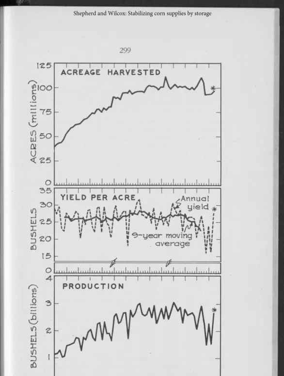
The way in which the acreage, yield and production o f corn has fluctuated from year to year since 1870 is shown in fig. 1.

The top section o f the chart shows that corn acreage does not change greatly from year to year. The greatest changes from one year to the next occurred in 1917 when, as a result o f heavy winter killing o f wheat, corn acreage rose 10 percent over the previous year, and in 1934 when, as a result o f extreme drouth and the A A A program, the acreage o f corn harvested fell 13 percent below the previous year. These years were excep­ tional. Ordinarily, corn acreage remains fairly constant.

The second section o f fig. 1 shows that the chief reason for fluctuations in the size o f the corn crop is changes in yield per acre. The effect o f these rather violent changes in yield, and o f the moderate changes in acreage, upon the total production o f corn is shown in the lower part o f the chart.

It is evident from fig. 1 that corn production fluctuates irregu­ larly and unpredictably from year to year, the average produc­ tion since 1900 being about 2.5 billion bushels. It is also evident that this fluctuation is not symmetrical above and below the aver­ age. The largest crops that have occurred since 1910 (when corn acreage stabilized out at about 100 million acres) have been about 3 billion bushels in size; this is 20 percent larger than average. O n the other hand, the smallest crops (the 1934 and 1936 crops) have been about 1.5 billion bushels in size; this is 40 percent smaller than average. That is to say, the size o f the crop fluctuates downward twice as far as it fluctuates upward. The largest crops run as much as 20 percent oversize, but the smallest crops run as much (o r should we say, little) as 40 per­ cent undersize.

W e have confined this statement to the period since 1910, be­ cause o f the complication introduced by the rising trend o f acreage before 1910. But the observation holds in a general way fo r the years before 1910 as well as after 1910. The smallest crops fall farther below the average than the largest crops ex­ ceed it. The very large crops are more numerous than the very small crops.

N

U

M

B

E

R

O

F

C

R

O

P

S

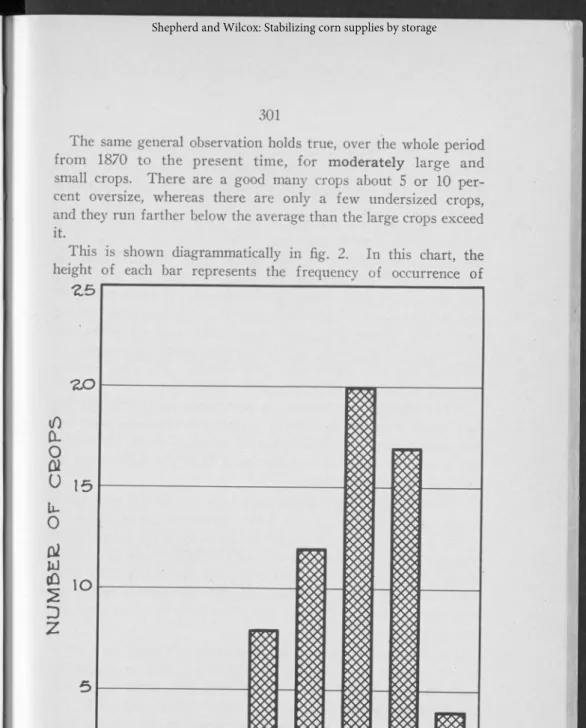
The same general observation holds true, over the whole period from 1870 to the present tim e, for m oderately large and small crops. There are a good many crops about 5 or 10 per­ cent oversize, whereas there are only a few undersized crops, and they run farther below the average than the large crops exceed it.

This is shown diagrammatically in fig. 2. In this chart, the height o f each bar represents the frequency o f occurrence o f

1 6 -

1 8 -

e o -

Z.7L- 'ZA-— 'ZQ>- Z Q -

3 0

-17.9 19.9 et.e *23.02.5.9 27.929 .9 3 1 . 9

AVERAGE YIELD OF CORN PER A C R E .

.UNITED S T A T E S

different sized corn crops. The size o f the corn crop is repre­ sented by the yield, since using yields frees the presentation from the complication resulting from the rising trend in acreage before 1910.

The average yield fo r the periods from 1870 to 1937 as a whole was 26 bushels per acre. The tallest bar in the chart shows that during this 68 year period there were 20 years in which the yield fell between 26 and 27.9 bushels per acre. The next bar to the right shows that there were 17 years when the yield fell between 28 and 29.9 bushels. The next bar to the right again shows that there were only 4 years when the yield was as high as 30 to 31.9 bushels, while there were no yields in any year higher than 31.9 bushels. The total number o f crops above average in size was 41.

In the other direction from the tallest bar, to the left, are the bars which show the number o f years when the crops were be­ low average in size. There were 27 o f these crops. The bars string out farther to the left than they do to the right, down to yields as low as 16 bushels.

This shows that the distribution o f the size o f the corn crops is not symmetrical above and below the mean but is “ skewed” to one side. That is to say, there are more large crops than small crops, in fact, 50 percent m ore; but the large crops exceed the average size less than the small crops fall short o f it. W e have numerous large crops, but they are only moderately large; we have only a few small crops, but when they do come they are very small.

It is also clear from the chart that large and small corn crops do not come in any simple or regular order, such as alternately from one year to the next. A big crop is as likely to be fol- ‘ lowed by another big crop as it is by a medium or small crop and vice versa. Corn crops come like heads or tails when a coin is flipped— sometimes alternately, sometimes two together, some­ times more than tw o in a string.

These characteristics o f corn crop fluctuations will be dis­ cussed in some detail at a later point in this bulletin, since they affect the way storage operations would work out in actual practice. But they are presented here merely as a part o f a pre­ liminary factual background approach.

X Z60

\f)

D 0 |_zoo, k. 1 0 Q) ISO 3 <0 5 IOO NEBRASKA I

f

vihLmk

f -

/

)lv T r

JJ..I.1 J * * * * * * * * * * * * * * * I 1 1 1 1 ...

4

1900 1906 19IZ 1906 191Z 19Z*4 1930 1936 500 4SO O , C 400 £ i 350 6 300 OHio

\ y

t»v

v\

hzkrh

-Ll.l, 1,1 ***** 1.11 II — i ***** L *1 1 * f \ ***** 1930 1936

GEOGRAPHICAL DIFFERENCES IN CORN

CROP FLUCTUATIONS

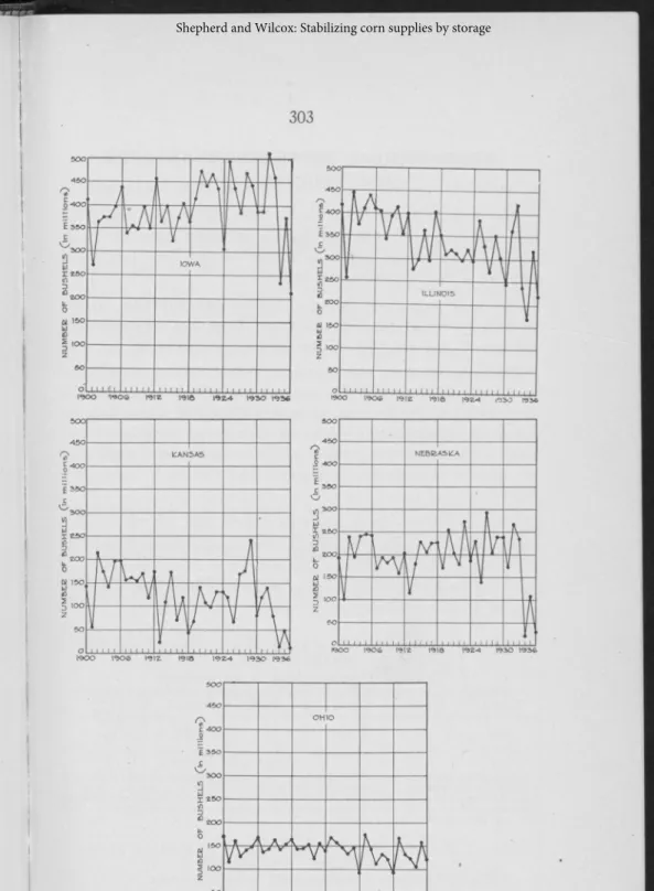
The greatest benefit from stabilization o f supplies would be realized in the areas where production fluctuates the most. These areas can be located by study o f the annual co m production data fo r a few representative states.2

The corn production data for Kansas and Nebraska on the western border o f the Corn Belt, fo r Iowa and Illinois in the heart o f it and fo r Ohio farther east are shown in fig. 3.3

These figures show that the most violent fluctuations in corn production are found in the states on the western margin o f the Corn Belt. In the central and eastern Corn Belt states the crop size is considerably more stable. A corn storage program, there­ fore, would have the greatest effect in stabilizing supplies in the western part o f the Corn Belt.4

2It would make a more sharply defined picture if type-of-farming areas were used here rather than states. But for preliminary purposes, states will suffice.

3Fig. 3 shows the extent of the fluctuations in each state, but it does not provide for very accurate comparisons. The differences in production levels and in trends up or dawn are confusing. The amount of fluctuations, however, can he summarized in a single figure for each state, and direct comparisons can be made by comparing these figures. These Summary figures are shown in table 1. They are the standard devia­ tions of the first differences between the data for successive years (which removes tne influence of trends) divided by the mean of the original production data (which con­ verts the figures to comparable percentage terms).

T A B L E 1. F L U C T U A T IO N S IN CORN P R O D U C T IO N IN V A R IO U S STATES, 1900-1936

(Coefficients of variation based on first differences)

Kansas Nebraska Iowa Illinois Ohio United_States

31.2 23.8 13.6 14.1 13.3 10.5

4Corn prices would be expected to fluctuate most in the- marginal statesi (where crop fluctuations are greatest). Summarizing the price fluctuations in a manner similar to table 1 shows, however, that they do not differ very greatly by states and that tne differences are not in all cases directly related to differences in crop fluctuations, lh e data are given in table 2.

T A B L E 2. F L U C T U A T IO N S IN CORN P R ICE S IN V A R IO U S STATES, 1908-1928, O M IT T IN G 1916-1919

(Coefficients of variation, based on first differences)

Kansas Nebraska Iowa Illinois Ohio United_States

m il l io n f e e d u n i t s

IMPORTANCE OF CORN AS A FEED CROP

H ow much would a stabilized supply o f corn contribute to stability in the total supply o f feed grains in the Corn Belt? In Iowa it is well known that corn is the most important crop, but it is not generally realized how important it is; in actuality, corn accounts fo r 70 percent o f all the feed (other than pasture) produced in Iowa. The great importance o f corn is shown in fig. 4 where total feed grain production (the solid line) fluctu­ ates sharply from year to year. The dotted line, showing the fluctuations in total feed grain production with corn production stabilized (at its trend value for each year) is much more stable. Computations show that over the past 36 years 75 percent o f the fluctuation in the total feed supply, including hay, in Iowa has been caused by fluctuations in corn production. T o put it the other way round— stabilizing corn supplies would remove 75 percent o f the fluctuation in total feed supplies.

The picture is similar in the North Central states.® Since . / T h i s is the name given to the western two-thirds or so of the Corn Belt plus ?£veivr fuato S outside the northwestern border of the Corn Belt. Specificallv N-?rth CAe/? tral include Ohio, Indiana, Illinois, Michigan, Wisconsin, Minne­ sota, Iowa, Missouri, North Dakota, South Dakota, Nebraska and Kansas

P E E C E N T A B O V E 4 & E L O W A V E B A G E

1900 there have been 14 years when the total feed grain pro­ duction was 10 percent or more either above or below average. This is shown in fig. 5. But with corn production stabilized at its average there is only one year, 1934, in the whole 37 year period when the fluctuation was as much as 10 percent above or below average.

Including hay along with the feed grains gives similar re­ sults. The fluctuations in total feed production including hay fo r the North Central states are shown in fig. 6. It is apparent that by stabilizing corn at its average all o f the extreme fluctua­ tions are greatly moderated. In evaluating the importance o f fluctuations in the feed supply in the Corn Belt which result from changes in hay production it should be kept in mind that total forage supplies are stabilized through the utilization o f more or less corn fodder, silage and straw. F or this reason fluctua­ tions in hay production are probably less important than they otherwise would be.

It is apparent that if corn could be stabilized through a stor­ age program great progress would be made not only toward

level-P E E C E N T A B O V E 4 B E L O W A V E E A G E 307

m g out the supply o f feed grains going to meat animals but also the total feed supplies going to all livestock in the Corn Belt.

INDIVIDUAL STORAGE IN THE PAST

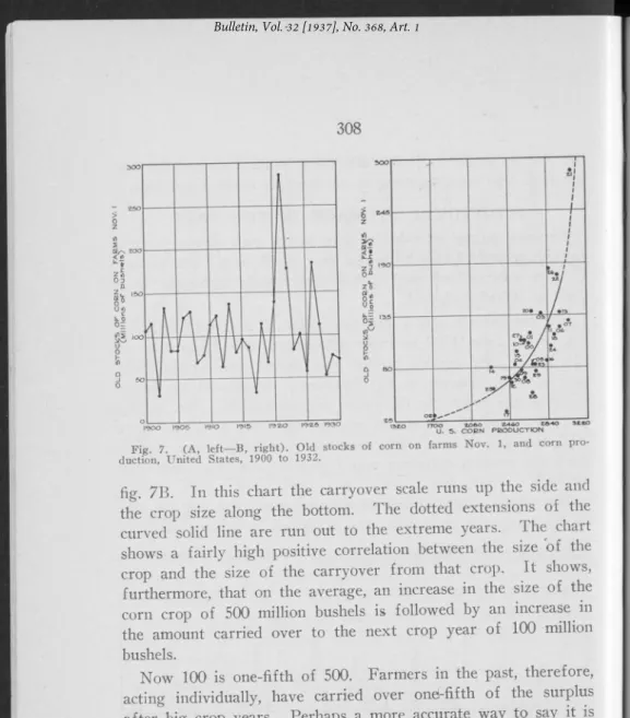
Farmers acting individually have in the past carried over a certain amount o f corn from one year to the next. T he amount o f corn thus carried over is shown in bushels each year from 1900 to 1930,6 in fig. 7A.

The carryover is only a small percentage o f the total c r o p ; over the period from 1900 to 1930, it averaged only 3.8 percent o f the crop. The amount carried over varied considerably from year to year, however, as fig. 7 A shows. In general, the larger the crop the larger the carryover, and conversely. The biggest carryover was 11 percent o f an average crop, after the large 1920 crop and the low prices resulting from the post-war depres­ sion; the smallest carryover was 1 percent, after the small crop

o f 1901. ' F

The relation between the size o f the corn crop and the size o f the carryover from that crop is shown in greater detail in

^ iter 1930 the date was changed from Nov. 1 to Oct. 1. The data after 1930 are therefore not comparable with the data before 1930. yJU are

308

fig.

7B.

In this chart the carryover scale runs up the side and the crop size along the bottom. The dotted extensions o f the curved solid line are run out to the extreme years. The chart shows a fairly high positive correlation between the size o f the crop and the size o f the carryover from that crop. It shows, furthermore, that on the average, an increase in the size o f the corn crop o f 500 million bushels is followed by an increase in the amount carried over to the next crop year o f 100 million bushels.

N ow 100 is one-fifth o f 500. Farmers in the past, therefore, acting individually, have carried over onel-fifth o f the surplus after big crop years. Perhaps a more accurate way to say it is th is: Farmers, by their storage actions, have reduced fluctuations in corn production by one-fifth. The fluctuations in consump­ tion and sale were only four-fifths as great as the fluctuations in production; the other one-fifth went into storage.

So a national corn storage program is not as revolutionary a proposal as it might seem. It merely proposes to carry further what has already been practiced fo r years on a small scale. There is this difference, however. Farmers carried corn over from large crop years in the hope o f profiting from fluctuations in p rices; the purpose o f a national plan is not to profit from price fluctuations but to smooth them out.

309

COSTS OF STORING CORN

In an economic world where everyone knew all about what to do and was free to do it, farmers would carry over corn from big crop years and dump it during small crop years to such an extent that price fluctuations would be greatly reduced. Prices would fluctuate only just enough to cover the costs o f storage.

It may be that farmers have been doing just that thing. It may be that any increase in storage operations would smooth price movements out so much that they would not cover storage costs, and the result would be a net loss. Let us see.

The first thing to do is to determine what these storage costs are.

The costs o f storage depend in large part upon where the grain is stored. In the past the bulk o f the corn was stored right on the farm where it was grown. Under a general storage plan, the bulk o f the corn would also be stored on the farm.

There are two or three reasons fo r this. The first reason is that just after harvest corn contains a high percentage o f mois­ ture. The limit o f moisture content fo r safe storage at the term­ inal elevators is about

17

percent in the winter and 13 percent in the summer. In the early winter Iowa corn ordinarily runs from 18 to 25 percent moisture. It would go out o f condition if shelled and put into terminal storage then.7

The corn could be safely stored if it were first artificially dried. But the operation o f drying costs from 2 to 4 cents a bushel and, in addition to this cost, the shipper bears the loss in weight from drying and general handling. Further, not only does commercial drying drive o ff the moisture, but (according to industrial users o f corn) fo r every 1 percent o f moisture driven off, about one- fourth o f 1 percent o f corn oil goes off with it. A nd finally, the process o f drying generally renders the grain unsatisfactory’ for industrial purposes, either because o f the starch being partly broken down or because o f the germ being killed. M ost industrial firms will not accept commercially dried co r n ; it must be disposed o f at a discount to feeders.

The second reason is that even if the corn were dry enough to store at the terminal the storage charges there are higher than

they are on the farm. (T h e amount o f the charges on the farm is given in detail later in this bulletin.) The unloading charge, which also includes 10 days free storage, is 1J4 cents a bushel. The storage charge thereafter is Ho cents a day, nearly

\y 2

cents a month. Shrinkage is not a factor here, however, since the same number o f pounds o f corn that were weighed into storage are weighed out.

The third reason is that the most strategic market location for Iowa corn is the farm where it was grown. There is some ad­ vantage in having grain in store at the terminal where it can be sold on a bulge at a moment’s notice, but grain on the farm in Iowa, surrounded as it is by a ring o f markets, is in a position to take advantage o f the highest on-track bids from perhaps a half dozen alternative sources at any time. Grain in store at a term­ inal market has to be sold there (o r else bear the cost o f ship­ ment to another m arket), though the original terminal market where it is located may never offer the highest price o f all the available markets during the period o f storage.

3 0

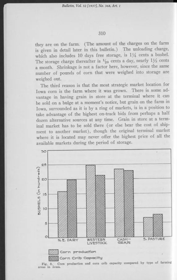
LIVESTOCK QEA1N

C orn production C orn C r ib C ap a city

Fig. 8. Com production and corn crib capacity compared by type o f farming areas in Iowa.

O 1 -2. 3 -4 5 G

AVERAGE CORN PRODUCTION (in thousands o f bushels')

Fig. 9. Relation between corn storage capacity and average corn production by individual farms, cash grain area of Iowa. (D ot numbers are farm serial numbers.)

FARM STORAGE SPACE

W e have seen that the best place to store corn is in the crib on the farm where it was grown. The cost o f storing corn there de­ pends upon several things. One o f the most important is the ade­ quacy o f the corn storage space already available on the farm.

A soil conservation survey o f 400 representative Iowa farms conducted during 1936 included the question o f the amount and condition o f corn storage space on farms. This survey showed that in each o f the type-of-farm ing areas o f the state the average amount o f corn storage on the farm was roughly equal to the av­ erage corn production per farm. This is shown in fig. 8. The basic data are given in table 3..

This does not mean that the amount o f corn storage on each farm was roughly equal to the average corn production on that farm. Figure 9, where each dot shows the amount o f corn stor­ age space and the average corn production for one farm, shows that there is only a rough correlation between the two. The cor­ relation is + 0 .5 5 . This is fo r the cash grain area. The situation in the other areas is similar.

Evidently some farms have considerably more storage space than average corn production, while others have considerably less.

This is partly accounted for by the variation in type o f farming from one farm to another, even within a given type-of-farm ing area.

A further point that requires consideration is the condition o f the cribs. Table 3 shows that only about half o f the cribs are in first class condition. A large proportion o f the cribs are rated 2, 3 or 4.

These things appear to point to the need fo r a considerable amount o f corn crib construction and repair. W hen many farms are underprovided with storage space, and a high proportion o f the cribs are in poor condition, a corn storage program o f some magnitude would call fo r extensive crib construction and repair. This work would be required not because a corn storage program would impose a great additional burden upon storage space (it is not often that we get a crop as large as 20 percent over average),

T A B L E 3. IO W A CORN ST O R A G E D A T A B Y S E C T IO N S.t Data _{dairy section}Northeast Western live­

stock section Cash grain section Southern pas­ture section Total number of farms... 171 108 109 117 Average com crib

capaci-ty in bushels (all types together) ... 1986 2137 2293 776 Number of owners... 87 40 35 51 Number of tenants ... 73 57 61 41 Number of owners and tenants ... 11 11 13 25 Average acres per farm... 176 189 168 194 Average corn crib

ca-pacity in bushels ... 1568 2454 2319 882 Combined crib and granary*. 3310 1696 2010 957 All other types, bushels

capacity ... 454 2709 503 Condition of crib Number “ good” ... 21 61 57 54 Number “ medium” ... 52 16 7 7 Number “ fair” ... 49 28 29 61 Number “ poor” ... ... 17 9 5 2 Present value corn crib... $246.00 $537.00 • $513.00 $259.00 Combined crib and granary... $441.00 $596.00 $733.00 $341.00 All other...,... $1488.00 $800.00 $714.00 Average corn production,

1935 (bushels) ... 1589 2484 2351 673 Average corn inventory, May

1936 (bushels) ... 398 377 437 92

tData for the eastern livestock area were not available in time for this study. *This figure shows the average corn capacity on those farms which had combined cribs and granaries. Practically no farms had both cribs and combined cribs and granaries.

but to put a large proportion o f the corn cribs into good repair, and to provide for only a relatively slight excess (10 or 15 per­ cent) above existing requirements.

CRIB COST

In cases where new cribs were required, the costs o f building and maintaining them should be considered. The crib cost is cal­ culated as made up o f two items— the interest on the investment and the depreciation or replacement charge.

The cost o f the crib will depend upon several things— the ma­ terial, the type o f crib and the care given it. The figure used in this discussion is based on the cost o f a common type o f crib. The cost o f any other type desired can be figured up in a similar manner and substituted.

A common type o f crib has a shingled, shed roof, concrete floor and crib boards on the sides. Such a crib, big enough to hold a sufficient amount o f ear corn to yield 1000 bushels o f shelled corn, would have a floor 8x32 feet, a rear height o f 10 feet and a front height o f 12 feet. The materials— lumber, ce­ ment and gravel— required to build a crib o f this size, at present retail prices in Ames, would cost approximately $185. Hardware, paint and labor would bring this figure close to $240. The annual interest on this, figured at 6 percent on half the original value (o n the basis o f straight-line depreciation), would be $7.20, or .7 cents a bushel per year.8

The annual replacement charge, assuming a normal life o f 40 years would amount to $6. W ith the crib filled to capacity (1000 bushels) the replacement charge would then be .6 cents a bushel per year. Finally, the insurance on the crib and corn at mutual rates would amount to about .4 cents a bushel per year. Thus the total annual cost o f the crib— interest on investment, de­ preciation and insurance— amounts to approximately 1.7 cents a bushel. Losses by rats and mice vary from farm to farm and are difficult to estimate in a single figure. I f we wish to use round numbers, we may take 2 cents a bushel per year as an approxi­ mately correct allowance to cover crib and insurance costs and losses from rodents.

8Anyone interested in detailed plans for corn cribs can secure them by writing to the Agricultural Engineering ■ Section of the Iowa Agricultural Experiment Station, Ames. Iowa.

The “ shrink,” or loss o f moisture o f the corn during storage, averages 9 or 10 percent during the first storage season. This loss in weight, however, is approximately offset by the higher price that the corn will command, because the reduction in mois­ ture content raises the grade o f the corn.

INTEREST GOST

The interest cost on a corn loan, secured by the corn as col­ lateral, would depend upon the amount o f the loan per bushel, the rate o f interest and the length o f time fo r which the corn would be stored.

The federal government made corn loans in 1933 and 1934 at 45 cents per bushel. In 1935 and 1936 the rate was 55 cents. In 1937 it was set at 50 cents. This figure, 50 cents, may be used as the basis o f our calculations.

The federal corn loan rate o f interest was 4 percent. I f corn were stored fo r a year, the interest cost on the basis o f these fig­ ures would be 2 cents per bushel.

TOTAL STORAGE COSTS

Under the most favorable conditions for profitable corn stor­ age— large crops alternating with small crops— the crib would be used every other year. The crib costs are overhead charges that run on whether co m is stored or not. Even under the most fav­ orable conditions then, 2 years’ crib costs would be charged to 1 year’s storage. The crib cost o f storing corn from a large crop to a short crop the next year would therefore be 4 cents per bushel. Added to this would be the 2 cents a bushel interest on the value o f the corn stored. The total storage costs fo r each storage operation would therefore be 6 cents per bushel.

Under actual conditions, as we saw in the early part o f this bulletin in fig. 1, corn crops do not alternate between large and small size from year to year. They come irregularly. A nd the large crops come one and a half times as frequently as small crops, exceeding average size only about half or two-thirds as much as small crops fall short o f average size.

This means that, on the average, corn would have to be stored from tw o large crops in succession.9 This would be the average

9W e saw earlier that there are SO percent more large crops (crops above average size) than small crops (crops below average size). Under a strict definition of aver­ age size, therefore, crops would on the average be stdred from one and a half large crops in succession. But there would be occasional crops of about average size when grain would be neither stored nor taken out of storage. These would increase the average length of time of grain storage to roughly 2 years.

situation. Quite frequently, o f course, there would be only one large crop, followed at once by a small crop, and quite frequently there would be three (o r even m ore) large crops in succession before a short crop happened along. But on the average the sur­ plus would have to be carried for 2 years and then dumped on a short crop year. The crib costs, being incurred every year whether corn was stored or not, would cover 3 years, amounting to 6 cents per bushel. The interest cost would be 1 cent the first year (since the crib would be only half filled) and 2 cents the second year, amounting to 3 cents altogether. The total cost for each storage operation would therefore be 9 cents per bushel.

In both o f these situations, the costs o f storage per year would be the same. The 6 cents for storing corn every other year would equal 3 cents per year; the 9 cents fo r storing corn every 3 years would also be 3 cents per year. The total storage costs, therefore, would on the average amount to 3 cents per bushel stored per year.

EFFECT OF SIZE OF CORN CROP UPON

HOG SUPPLIES

W e have seen that the cost o f storing corn averages about 3 cents per bushel stored per year. W hat now would be the gains from storing corn ? W ou ld they be more or less than the costs?

In order to answer this question, we have to consider first what the effects o f fluctuations in corn production have been in the past; that will show, in reverse as it were, what the gains would be from smoothing them out.

Only a small percentage o f the corn crop is sold as cash grain, about 85 percent o f the corn produced in Iowa being fed to live­ stock in the county where it was grown. The percentage fo r the Corn Belt as a whole is not far from the same figure. The most important effects o f fluctuations in corn production, therefore, are those which show up in the livestock industry.

In Iowa, hogs are the chief source o f income to farm ers; they bring in over 40 percent o f the total income. Cattle come next, contributing about 16 percent.10 F or simplicity, most o f our dis­ cussion o f livestock will run in terms o f the largest item, hogs.

lOBasebook of Iowa, Special Report No. 1, Iowa Agr. Ec. Subsection and Extension Service Cooperating, pp. 9-10, 1936.

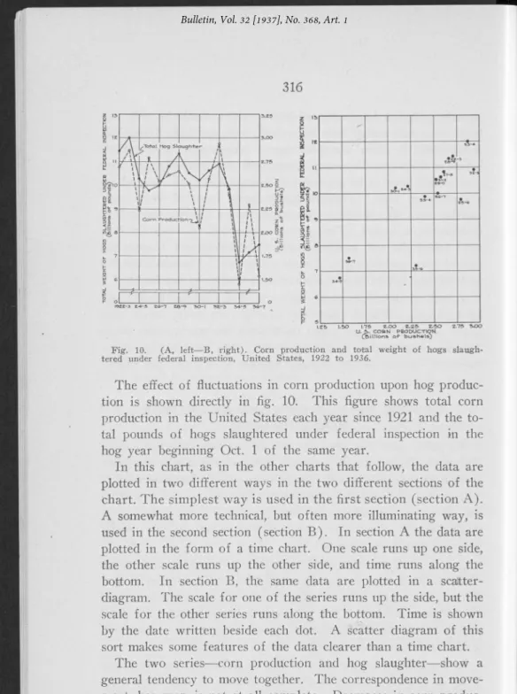
Fig. 10. (A , left— B, right). Corn production and total weight of hogs slaugh­ tered under federal inspection, United States, 1922 to 1936.

The effect o f fluctuations in corn production upon hog produc­ tion is shown directly in fig. 10. This figure shows total corn production in the United States each year since 1921 and the to­ tal pounds o f hogs slaughtered under federal inspection m the hog year beginning Oct. 1 o f the same year.

In this chart, as in the other charts that follow, the data are plotted in two different ways in the two different sections o f the chart. T h e sim plest w a y is used in the first section (section A ) . A somewhat more technical, but often more illuminating way, is used in the second section (section B ). In section A the data are plotted in the form o f a time chart. One scale runs up one side, the other scale runs up the other side, and time runs along the bottom. In section B, the same data are plotted in a scaJtter- diagram. The scale fo r one o f the series runs up the side, but the scale fo r the other series runs along the bottom. Tim e is shown by the date written beside each dot. A scatter diagram o f this sort makes some features o f the data clearer than a time chart.

The tw o series— corn production and hog slaughter— show a general tendency to move together. The correspondence in move­ ment, however, is not at all complete. Decreases in corn produc­ tion are followed at once by decreases in hog slaughter, but marked increases in corn production take more than a year to show up in hog slaughter.

The reason for this is clear. Farmers can reduce the total weight o f their hog slaughter very quickly when the corn crop is small, as it was in 1924 and 1934, But once the hogs are gone, and a big crop comes along, hog slaughter cannot snap back to full capacity at on ce; it takes more than a year to build up the herd again. This is particularly true if the increases are large. A small increase in corn production will be taken care o f by feed­ ing hogs to heavier weights, but a large increase can only be taken care o f by heavier breeding, which cannot show up until the next hog crop year.

H ow can this be taken into account in our charts? One way would be to lag the hog slaughter series a year after the corn production series. But this would shift the whole series, whereas it is only the years o f large increases in corn production that need to be dealt with. A nd it would ignore the size o f the cur­ rent corn crop each year. W hat is needed is to identify the years when large increases took place in corn production, and in those years only, to average up the large crop with its predecessor.11 W e may define a large increase as one over 10 percent. There are 4 such years— 1925, 1931, 1932 and 1935.

The effect o f handling the corn production data in this man­ ner for these 4 years is shown in fig. 11. The commanding in-P-A weighted average is used, giving the preceding year twice the weight of the current year.

Fig. 11. (A, left— B, right). Corn production and total weight o f hogs slaughtered under federal inspection, United States, 1922 to 1936. Large corn crops averaged with preceding crops.

fluence o f corn production upon hogs slaughtered is clearly shown in section A .

Section B shows the same thing, the closeness o f the relation being indicated by the closeness with which the dots lie along the sloping line drawn through them.12 The chart shows further­ more that a change in corn production o f 250 million bushels is associated with a change in the total weight o f hogs slaughtered o f 10 billion pounds. These quantities represent about 10 percent in both cases. The relationship, therefore, is 1 to 1— a change in corn production results in an equal percentage change in hog supplies.

EFFECT OF SIZE OF HOG CROP UPON HOG PRICES

W e are now ready to consider the next link in the chain o f cause and effect.

The changes in hog supplies shown in fig. 11. in turn cause marked changes in the opposite direction in hog prices. This effect is definite and clear-cut during periods when the demand fo r hogs is stable.13

The demand during the period from 1922 to 1929 was reason­ ably stable. The hog supplies and prices each year from 1922 to 1929, inclusive, are shown in fig. 12. The inverse correlation be­ tween hog supplies and prices is clearly shown. The only year when a change in supplies did not result in an opposite change in prices is 1928-29. This was the peak o f the boom before the depression that began late in 1929. The strong demand in that year more than offset the depressing infiuence o f larger hog sup­ plies upon prices. In addition, cattle numbers were at the bot­ tom o f their cycle in 1928.

The sequence o f causation, then, is comparatively sim ple: A n increase in corn supplies causes a corresponding increase in hog supplies, and this increase in hog supplies causes a decrease in hog prices.

Figure 12 shows that hog prices fiuctuate more violently than hog supplies. A change in hog supplies causes a considerable greater

120 ne could go further, and use a weighted average of the com current year and the preceding year for years of marked decreases as well as for marked increases. The average in this case should about 2 to the current year, instead of to the preceding year.

iSWhen the demand for hogs is changing violently, however, as onward through the depression, the effect of these changes in hog obsefures the effect of changes in hog supply. H og supplies push down the same as ever, but the push is (more or less) offset or effect of changes in demand.

production in the (over 10 percent) give a weight of it did from 1930 demand partially hog prices up or added to by the

change in hog prices. Figure 12B shows more clearly than fig.

12A that the change in hog prices is nearly twice as great as the change in hog supplies that caused it. The chart shows that a change in hog slaughter o f 1 billion pounds causes a rise in hog prices o f nearly $2 per 100 pounds. This can be stated in per­ centage terms: A change o f 10 percent in hog supplies, for e x ­ ample, causes an opposite change in prices o f nearly 20 percent. I f the relationship were 1 to 1— if a change o f 10 percent in hog supplies caused an opposite change in hog prices o f an equal amount (10 percent)— the change in the one would approxi­ mately offset the change in the other, and the total income would remain roughly constant, unaffected by changes in supplies.

But, as fig. 12 shows, the change in hog prices is nearly twice as great as the changes in hog supplies that caused it. The total income, therefore, fluctuates with (o r rather, conversely with) hog supplies. The effect upon the total income can be shown by tak­ ing the original data fo r a few representative large and small crop years.

The corn crop in 1923, fo r example, was large; it amounted to 2.9 billion bushels. The total weight o f hogs slaughtered in the hog year October 1923 to September 1924 was correspond- ingly large, it totaled 12 billion pounds. The price o f hogs was correspondingly low, only $7.41 per 100 pounds live weight. The

r'

V

o g P r 1

\

Y

\/

/ 1

o g S la t " 3?_{2l 5} BCi h to p§ f t0. 5 ZO ST _P®*“ pjio in « gì 0 S O 0 E S °§ Ô < 0 » 7 S ’ < 0 ^ 7 \. \zs-i

\

t*-7\ • \ 19*0 \ 1»' t«-9 MrS \ T O T A L. LIVE W EIGHT O F H O G S S L A U G H T E R E D L3NDEB F E D E R A L IN S P E C T IO N

• . 12‘ w L left B> ri&ht). Total live weight of hogs slaughtered under federal inspection, and average hog prices, United States, 1922 to 1930.

total income from the sale o f hogs, therefore, was 12 billion multi­ plied b y $7.41/100, w h ich equals 889 m illion dollars.

Then came the short corn crop o f 1924. Because the crop was small, the price o f corn was high, and heavy liquidation o f un­ finished hogs resulted late in 1924. H og slaughter for the 1924- 25 hog year was reduced to 10.3 billion pounds which sold at a price o f $11.18. The total income from this small hog crop was 10.3 billion m ultiplied b y $11.18/100 w h ich equals 1,151 m illion dollars. T h e total incom e from the small h o g crop w as m a­ terially higher than the total income from the preceding year’ s large hog crop.

This sounds strange, indeed, almost perverted. But that is the case with most staple foods. I f they are scarce, people will pay high prices rather than turn to something else. Economists sum­ marize this sort o f situation in a phrase by saying that the demand is inelastic.

EFFECT OF SIZE OF HOG CROP UPON THE TOTAL

VALUE OF THE CROP

The corn crops in 1934 and 1936 were still smaller than the crop in 1924. They showed up in severe reductions o f hog sup­ plies. The effects o f these reduced hog supplies upon hog prices were complicated by the changes in demand that were taking place at the same time (during recovery from the depression) and can­ not be shown in one simple chart. These changes in demand, however, can be taken into account by the use o f technical sta­ tistical methods. A n analysis made with the use o f these methods is shown in Appendix A . This analysis shows that over the en­ tire period from 1922 to 1936 the general relationship between hog supplies and prices is th is: W hen hog supplies change 10 percent, hog prices change (in the opposite direction) 16 per­ cent.14 H o g prices change more than hog supplies; that is why a small crop o f hogs is worth more than a large crop.

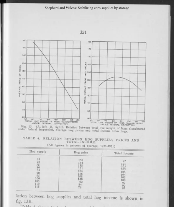
The general relation between hog supplies, prices, and total income, can be set forth as in table 4. F or simplicity, the figures used are percentages, with 100 representing average size. The re­ lation between hog supplies and prices is shown in fig. 1 3A ; the re-l4For hog crops smaller than 80 percent of average size, the effect on prices is less than this. The demand ciurve is not quite straight- but is Slightly curved, convex upwards.

T A B L E 4. R E L A T IO N ^ J ^ ^ Ç nC O M E 8111,1,01^8, P R ICE S A N D (All figures in percent of average, 1921-1931)

H og supply _{H og pr} 65 ₁₅₀ 70 ₁₄₄ 75 ₁₃₈ 80 ₁₃₁ 85 ₁₂₄ 90 ₁₁₆ 95 ₁₀₈ 100 ₁₀₀ 105 ₉₂ 110 ₈₄ 115 ₇₆ Total income 97 101 103 105 105 104 103 100 97 92 87

lation between hog supplies and total hog income is shown in fig. 13B.

Table 4 shows that a large crop o f hogs is worth less than a small crop. It shows that a 110 percent crop, fo r example, brings a total income qnly 92 percent o f average, but a 90 percent crop brings a total income 104 percent o f average. The large crop o f hogs is worth 12 percent less than the small crop.

I f we consider still larger and smaller crops, the difference be­ tween their total values is still greater. A 115 percent hog crop brings an 8

7

percent income, which is 18 percent less than the in­ come from an 85 percent crop. The rise in total income with

decreasing size o f crop, however, ceases below „crop sizes o f about 83 percent.

The fact that a large crop o f hogs is worth less than a small crop is a very significant finding from the point o f view o f farm management. It means that when the corn crop is large, and corn prices and total incomes are low, farmers as a group do not escape the effect o f these low corn prices and incomes by feeding the corn to livestock more heavily; they merely translate it into lower hog prices and incomes a year or two later. The decrease in hog prices and total incomes is approximately equal to the de­ crease in corn prices and incomes.

FLUCTUATIONS DEPRESS AVERAGE INCOMES

A final conclusion is also important. The two total income fig­ ures fo r the 115 and 85 percent hog crops were 87 and 105, re­ spectively. N ow if you add up these two total income figures and divide by 2 you get less than 100; you get only 96. That is, the total income from the sale o f tw o hog crops, one o f them large and the other small, averages less than the in com e,from tw o average size crops. Fluctuations in hog supplies not only un­ stabilize hog sale incom es; in addition, they reduce them. The total income from a series o f large, average and small hog crops is less than the total income from a series o f average size hog crops.15

A national storage program for corn, therefore, that would con­ vert large and small hog crops into a series o f average sized crops, would not only stabilize hog prices and hog sales incom es; over a period o f years it would raise hog incomes as well. The in­ crease would be slight (only 2 percent) fo r fluctuations in hog crops o f 10 percent above and below average. But fo r fluctua­ tions. o f 15 percent above and below average the increase would be 4 percent, and fo r fluctuations o f 20 percent the increase would be 7 percent or more.

EFFECT OF A CORN STORAGE PROGRAM UPON

CASH CORN

W e turn now to consider the effects o f a corn storage program upon that small part o f the corn crop (15 percent) that is sold as cash grain.

In some ways these effects are more clear-cut than those upon the hog industry; they can be computed directly from the annual corn production and corn price data. In other respects, however, the effects are less clear.

One o f the reasons fo r this is that corn prices are determined not only by changes in supply and in the general demand fo r ag­ ricultural products but also by changes in the number o f live­ stock in the country; there are three independent determinants o f corn prices. This makes it impossible to show the effects o f corn production directly upon corn prices by plotting the original data in a simple chart, even fo r the comparatively stable period from 1922 to 1929 that was used in

fig.

12 to show the relation between hog supplies and prices. This difficulty, however, is pure­ ly statistical. It is taken care o f in the statistical analysis o f the factors determining corn prices, given in Appendix B. The re­ lation between corn supplies and prices revealed by this analysis is very similar to the relation between hog supplies and prices that was shown in fig. 13.

This means that in the case o f corn, as in the case o f hogs, a small crop is worth more than a large crop. The number o f bushels is less, but the price is so much higher that the result is a higher total value than that o f a large crop. This is true for crops down to about 83 percent o f the average.

In the case o f hogs, we multiplied the total slaughter by the average price, each year, to get the total income. In the case o f corn, however, we cannot do this; all the hogs slaughtered are sold as hogs, but only a small percentage o f the corn produced is sold as cash corn. This is the other respect in which the effect o f corn supplies on corn prices is less clear-cut than the effect o f hog supplies on prices. The difficulty here is not statistical; it is conceptual. The total value figures fo r corn, obtained by multi­ plying the production by the December price, do not show total sales income, but only imputed total value.

There are two ways o f thinking this thing through accurately. One is to note that the percentage o f the corn crop that is sold as corn is fairly constant from year to year, fo r the stafe o f Iow a16 and presumably fo r other parts o f the Corn Belt, too. One would be on reasonably safe ground, then, if he multiplied the price o f corn each year, not by total corn production, but by 15 percent o f the total production. That would show approximately the total income from cash corn sales each year.

The other way o f thinking through this situation is to consider- that although the bulk o f the corn crop is not sold as corn, the corn crop as a whole for the average farmer has approximately the same value whether it is all fed to livestock or all sold as corn. This must be true, since if at any time corn was worth more as cash corn than its imputed value if fed. to livestock, farmers would sell more and feed less; and this would bring cash corn prices down to equality with the imputed value o f corn fed to livestock.

This is not theorizing; it is a fact. The total value o f the corn crop fluctuates closely in accordance with the actual value o f the hogs to which it is fed. This is shown in fig 14A, where the total

iSBentley, R. C., Destination of Iowa’ s Commercial Corn. Iowa Agr. Exp. S > Bui. 318, p. 6, table 1. 1935.

value (production times price) o f the corn crop is plotted with the total value (slaughter times price) o f the corresponding hog crop .17

Both o f these series show the effects o f the depression after 1929. Indeed, part o f the positive correlation between them re­ sults from the similarity o f their responses to the depression. In order to remove these depression effects, both series should be divided through by an index o f demand. The index o f total non- agricultural income for the United States is used for this purpose. The results o f dividing the items in each series by the corres­ ponding index o f demand each year18 is shown in fig. 15.

It will be observed that the line in fig. 14B (and in. fig. 15B also) which represents the relationship o f corn values and hog values, has a slope o f about 1 to 1. This means that the changes in corn crop and hog crop values are not only closely related, they

l^The corn crop values are given in Agricultural Statistics, 1937, p. 39, in the col- umns headed Farm value.” A two year moving average of the value figures is used; tnat is, each total corn value item plotted in fig. 14 is the average of the current and preceding yejar. It is a weighted average; the preceding year is given a weight of two, and the present year a weight of one.

. hog croP values are computed by multiplying1 the total live weight of the hogs slaughtered each month by the average cost of packers for that month, and adding up the twelve products October to September for each hog year. These data are given in Livestock, Meats and W ool Market Statistics,” 1937, pp. 164-165.

l8The analysis in Appendix A shows that this index of demand does not have a 1 to 1, nor even a constant, relationship to hog prices. Accordingly, the division is performed, not by the index, but by the effect which that index has upon hog prices. I f in a certain year the index stood at 90, one would read up from 90 on the hori- ZOntu Appendix A , fig 19A, to the curved line, then across from that point on that line to the left hand scale, and divide by that figure .

are also approximately equal in amount. A 10-percent change in corn crop values is associated with a 10 percent change in hog crop values, a 20 percent change in corn crop values with a 20 per­ cent change in hog crop values and so on.

W OULD A CORN STORAGE PROGRAM STABILIZE

CORN PRICES?

W e have shown the effects o f fluctuations in corn production. The question now arises: W ou ld a national storage program smooth them out? I f a large crop were reduced to average size by withholding o f the surplus, would the price rise to average crop size levels, or would it remain depressed by the fact that the surplus corn was still in existence?

Let us use concrete figures. Suppose that the demand fo r corn stood at a level such that an average size corn crop o f 2.5 billion bushels sold fo r 60 cents per bushel at the farm. Under these conditions, a bumper crop o f 3 billion bushels (20 percent over­ size) would depress the price to 40 cents a bushel.

Suppose then that a corn storage program were put into effect, and that it was decided to store all o f the surplus (the amount above an average cro p ). I f there were no uncertainty as to the practicability o f the program— if people in general expected the administrators to carry through their announced intention o f with­ holding all o f the surplus— the large crop would be converted, in effect, to an average size crop. The question is : In that case, would the price o f corn rise to 60 cents a bushel, or would it stay down at 40? W ou ld the half billion bushel surplus still “ hang over the market” and depress prices anyhow?

The answer to this question is evidently no. I f all o f the sur­ plus corn were stored, the amount fed to hogs that year would be only 2.5 billion bushels, equal to an average corn crop. The size o f the hog crop and the price o f hogs the next year would therefore be the same as from an average corn crop. Farmers, anticipating this, would bid corn prices up to average corn and hog production levels. One might summarize this by saying that it is the amount o f a commodity consumed that sets its price, not the amount produced.

The question as to the effect o f a storage program on prices would be chiefly academic if the program were put into effect, as

it has been in past years, by means o f loans at a definite fixed figure per bushel above the natural market price fo r a large crop. Then the mechanism would work the opposite from normal. In­ stead o f the amount consumed determining the price, the loan value would set the price, and that would determine the amount consumed. I f the intention o f the administrators were to stabilize the price at 60 cents, instead o f deciding to store half a billion bushels from the large crop and trusting that that would raise the price to 60 cents, they would reverse the process. They would set the loan value at 60. cents and expect that that would result in the storage (i. e., the non-sale) o f a half billion bushels.

HOG PRODUCTION COSTS ARE INCREASED BY

FLUCTUATING CORN SUPPLIES

W e have been discussing the effects o f fluctuations in corn pra- duction upon co m and hog prices and total incomes. W e turn now to consider their effects upon livestock production costs.

During the past 10 years, the total weight o f hogs slaughtered annually has varied from 11.3 billion pounds in 1928-29 to 6.7 billion pounds in 1934-35. These annual variations in hog pro­ duction increase both the cost o f hog production on the farm and the cost o f transporting, processing and distributing the pork. A farm, transportation and processing plant that is equipped to handle more than 11 billion pounds must have many o f its parts idle and unemployed when less than 7 billion pounds are produced and processed.

Morever, changes in total slaughter fo r the United States tell only a small part o f the story. The total figures are the significant ones fo r price and total income analysis; but they do not reveal the changes that are important fo r the study o f costs o f produc­ tion. A drouth may reduce the size o f the corn crop 10 percent, and that may reduce total hog slaughter 10 percent the next hog year. But drouth never strikes evenly over the whole country; it is always more severe in some parts than others. In some areas the corn crop that year (and therefore the hog crop ) may have been reduced 20, 30, 40 percent or more. W e saw early in this bul­ letin (table 1) that the average fluctuation in corn production in any one state is greater than fo r the United States as a whole— ■ about 30 percent greater in Iowa, Illinois and Ohio, about 100

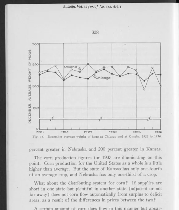
DEC EMB ER AVEB AGE WE IGHT O F H O G S

Fig. 16. December average weight of hogs at Chicago and at Omaha, 1922 to 1936.

percent greater in Nebraska and 200 percent greater in Kansas.

The corn production figures for 1937 are illuminating on this point. Corn production fo r the United States as a whole is a little higher than average. But the state o f Kansas has only one-fourth o f an average crop, and Nebraska has only one-third o f a crop.

W hat about the distributing system fo r corn ? I f supplies are short in one state but plentiful in another state (adjacent or not far away) does not corn flow automatically from surplus to deficit areas, as a result o f the differences in prices between the tw o?

A certain amount o f corn does flow in this manner but appar­ ently only enough to alleviate the differences in supplies to a small extent, not enough to remove them. Corn supplies are quickly reflected in average weight o f hogs marketed. The figures for Omaha, which serves an area o f variable corn crops, and Chicago, which draws from a wider and more stable territory, are illuminat­ ing. They are shown in fig. 16. They show that the flow o f corn to short crop areas is so inadequate to even out supplies that great differences still exist between the average weights, year by year, in the two markets.

The same situation is revealed by the statistics fo r Iowa. F ig­ ure 17 shows the number o f hogs 9 months old and over assessed from 1929-1937 in 21 southern Iowa counties. These counties suffered a serious drouth in both 1934 and 1936.. In January 1937 hog numbers were less than one-third o f what they had been 3 to 5 years earlier. A study o f 41 o f the better livestock farmers in better than average financial positions in this area shows that they produced only 55 percent as many hundredweights o f hogs in 1937-38 as they had produced in 1932-33.

• EFFECT OF FIXED COSTS

H og production costs are divided on a percentage basis about as fo llo w s : feed 75 to 85 percent, other costs (such as veterinary which vary directly with the number o f hogs produced) 5 to 10 percent, fixed costs such as interest on buildings and equipment, 10 to 15 percent.19 I f the hog producing plant is equipped to produce 10 billion pounds but is utilized to produce only 8 billion pounds, the cost per pound will be raised by about 3 percent, be­ cause the total overhead costs run on as large as ever, but are spread over fewer hogs. Costs per pound g o up proportionately more as the hog crop decreases, until the excessive overhead costs l 9Hopkins, John A. W h y H og Profits Vary. Ia. Agr. Exp. Sta., Bui. 255, 1929. .

Fig. 17. Number of swine 9 months old and over assessed in 21 southern Iowa counties, 1929 to 1937.

on a crop half as large as normal in any area result in 10 to 15 percent higher costs per pound than hog crops that fully utilized the fixed investment in the hog producing plant.

W ith the production o f corn only one-fourth or one-third o f normal in Kansas and Nebraska in 1937, the inevitably small crop o f hogs marketed from these states will have to carry unusually high overhead costs. On the other hand in large hog crop years, such as 1928-29, when 11.3 billion pounds o f hogs were marketed, the capacity o f the existing plant must have been overtaxed and much overtaxed in the areas o f heaviest production. N o doub| more than the usual number o f sows farrowed in inadequate quarters, excessive crowding resulted from