Journal of Modern Applied Statistical
Methods
Volume 13 | Issue 2 Article 18
11-2014
Ridge Regression and Ill-Conditioning
Ghadban Khalaf
King Khalid University, Saudi Arabia, [email protected]
Mohamed Iguernane
King Khalid University, Saudi Arabia, [email protected]
Follow this and additional works at:http://digitalcommons.wayne.edu/jmasm
Part of theApplied Statistics Commons,Social and Behavioral Sciences Commons, and the
Statistical Theory Commons
This Regular Article is brought to you for free and open access by the Open Access Journals at DigitalCommons@WayneState. It has been accepted for Recommended Citation
Khalaf, Ghadban and Iguernane, Mohamed (2014) "Ridge Regression and Ill-Conditioning,"Journal of Modern Applied Statistical Methods: Vol. 13: Iss. 2, Article 18.
Dr. Khalaf is an Associate Professor in the Department of Mathematics. Email him at
[email protected]. Dr. Iguernane is an Assistant Professor in the Department of Mathematics. Email him at [email protected].
Ridge Regression and Ill-Conditioning
Ghadban KhalafKing Khalid University Saudi Arabia
Mohamed Iguernane King Khalid University Saudi Arabia
Hoerl and Kennard (1970) suggested the ridge regression estimator as an alternative to the Ordinary Least Squares (OLS) estimator in the presence of multicollinearity. This article proposes new methods for estimating the ridge parameter in case of ordinary ridge regression. A simulation study evaluates the performance of the proposed estimators based on the Mean Squared Error (MSE) criterion and indicates that, under certain conditions, the proposed estimators perform well compared to the OLS estimator and another well-known estimator reviewed.
Keywords: Ordinary Least Squares, ill-condition, ridge regression, simulation.
Introduction
In regression problems the goal is usually to estimate the parameters in the general linear regression model
Y Xe (1)
where Y is an (n × 1) response vector, X is an (n × p) matrix of n observations of p predictors. It is important to note that X is not a square matrix since the number of data values n is usually larger than the number of predictors of p. β is an (p × 1) vector of unknown regression parameters, and e is an (n × 1) vector of the random noise in the observed data vector Y, it is often assumed that they are distributed as Gaussian with E(e) = 0 and Var(e) = σ2.
However, a method is needed to estimate the parameter vector β. The most common method is the least squared regression by finding the parameter values which minimize the sum of squared residuals, given by
RIDGE REGRESSION AND ILL-CONDITIONING
2
SSR
YX (2)The solution turns out to be a matrix equation, defined by
1
ˆ (X X) X Y
(3)
where X' is the transpose of the matrix X and the exponent (−1) indicates the matrix inverse of the given quantity.
It is expected that the true parameters will provide the most likely result, so the least squares solutions, by minimizing the sum of squared residuals, gives the maximum likelihood values of the parameters vector β. It is known from the Gauss-Markov theorem that the least squares estimate results the best linear unbiased estimator of the parameters; thus, this is one reason why least squares method is very popular. The estimates of the least squares are unbiased (i.e., the expected values of the parameters are the true values), and of all the unbiased estimators, it gives the least variance.
However, there are cases for which the best linear unbiased estimator is not necessarily the best estimator. One pertinent case occurs when the two (or more) of the predictor variables are very strongly correlated. In other words, when terms are correlated and the columns of the design matrix X have an approximate linear dependence, the matrix (X'X)−1 becomes close to singular. As a result, the least squares estimate, given by (3), becomes highly sensitive to random errors in the observed response Y, producing a large variance. To solve this problem, one approach is to use an estimator which is no longer unbiased, but has considerably less variance than the least squares estimator.
Ridge Regression and Multicollinearity
Ridge Regression is a technique for analyzing multiple regression data that suffer from multicollinearity. When multicollinearity occurs, least squares estimates are unbiased but their variances are large so they may be far from the true value, deflate the partial t-test for the regression coefficients give false non-significant p-values and degrade the predictability of the model. Thus, by adding a degree of bias to the regression estimates, ridge regression reduces the standard errors and the matrix needed to invert no longer has a determinant near zero; therefore, the solution does not lead to uncomfortably large variance in the estimated parameters. Now, given a response vector Y and a predictor matrix X, the ridge regression coefficients are given by
1ˆ k X X kI X Y
(4)
where k is the ridge parameters and I is the identity matrix. When k = 0, the linear regression estimate is given by (3), and when k = 1, ˆ( ) k 0, finally, for k in between, two ideas are balanced: fitting a linear model of Y on X’s and shrinking the coefficients. Small positive values of k improve the conditioning of the problem and reduce the variance of the estimates. While biased, the reduced variance of ridge estimates often result in a smaller MSE when compared to least squares estimates.
The amount of shrinkage is controlled by k, the ridge parameter that multiplies the ridge penalty. Large k means more shrinkage, thus, different coefficient estimates are obtained for different values of k. In fact, choosing an appropriate value of k is important and also difficult, but it can be shown that there exists a value of k for which the MSE (the variance plus the bias squared) of the ridge estimator is less than that of the least squares estimator. As a result, under the condition of multicollinearity, a huge price is paid for the unbiasedness property that is achieved by using the OLS estimator.
Choosing the Ridge Parameter k
One of the main obstacles in using ridge regression is in choosing an appropriate value of k. For selecting the best ridge estimator, several criteria have been proposed in the literature (see for example; Hoerl & Kennard, 1970; Hoerl et al., 1975; Hoerl & Kennard, 1976; Lawless & Wang, 1976; Gibbons, 1981; Saleh & Kibria, 1993; Troskie & Chalton, 1996; Kibria, 2003; Khalaf & Shukur, 2005;
Dorugade & Kashid, 2010; and Khalaf, 2013). Next, some formulas for determining the value of k to be used in (4) are discussed.
Hoerl and Kennard (1970) suggested using a graphic which they called the ridge trace. This plot shows the ridge regression coefficients as a function of k. When viewing the ridge trace, the value of k is chosen at which the regression coefficients have reasonable magnitude, sign and stability, while the MSE is not grossly inflated. In fact, letting βmax denote the maximum of the Βi, Hoerl and
Kennard (1970) showed that choosing
2 2 max ˆ ˆ ˆ k (5)
RIDGE REGRESSION AND ILL-CONDITIONING implies that 2 1 1 ˆ ˆ ˆ ( ( )) ( ) p i i MSE k MSE t
, where ˆ2 is the usual estimator ofσ2, defined by ˆ2 ( ˆ) ( ˆ) 1 Y X Y X n p
. The estimator, given by (5), will be
denoted by HK.
Hoerl, Kennard and Baldwin (1975) argued that a reasonable choice of k is
2 p k
(6)if these quantities were known. They suggested using
2 ˆ ˆ ˆ ˆ p k
(7)as an estimate of k in (6). This ridge estimator will be denoted by HKB.
Hoerl and Kennard (1976) proposed an iterative method for selecting k. This method is based on the formula given by (7). To obtain the first value of k, they used the least squares coefficients. This produces a value of k. Using this new k, a new set of coefficients is found, and so on. In fact, this procedure does not necessarily converge.
Lawless and Wang (1976) concluded that the ridge estimators using (5) and (7) performed very well indeed and that they were substantially better than any of the other estimators included in their study. Gibbons (1981) conducted a simulation study to compare 10 promising algorithms for selecting k. She found too that the estimators using the ridge estimator given by (7) performed well. In the light of these remarks, which indicate the satisfactory performance and the potential for improvement of the estimators HK and HKB, new methods are proposed to determine ridge parameter in case of ordinary ridge regression for the ridge parameter k as
1) KIa = The Arithmetic Mean of (HK, HKB)
2 2 max ˆ 1 ˆ ˆ ˆ 2 p (8)
2) KIh = The Harmonic Mean of (HK, HKB) 2 2 max ˆ 2 2 ˆ ˆ 1 1 ˆ HK HKB p
(9)3) KIg = The Geometric Mean of (HK, HKB)
2 2 max ˆ . ˆ .ˆ ˆ p HK HKB (10) 4) KIs The sum of ( , ), if 1 The sum of ( , ) / 2, if 1 HK HKB HK HKB HK HKB HK HKB . (11)
If the resulting HK+HKB, given by (11), is less than one, then it is used as an estimator for the ridge parameter k. However, if the resulting HK+HKB is greater than or equal to one then the new value of the ridge parameters equal to the value of (HK+HKB) divided by two.
Simulation Study
A simulation study was conducted in order to draw conclusions about the performance of the proposed estimators relative to HK, HKB and the OLS estimator. To achieve different degrees of collinearity, following Kibria (2003), the independent variables were generated by using the following equation
12 2
1 , 1, 2,..., 1, 2,...,
ij ij ip
x
z
z i n j p (12)where zij are independent standard normal distribution, p is the number of the
explanatory variables and ρ is specified so that the correlation between any two independent variables is given by ρ2. Four different sets of correlation were
considered according to the value of ρ = 0.7, 0.9, 0.95 and 0.99.
The other factors varied were sample size (n) and the number of regressors (p). Models consisting of 15, 25, 50 and 100 observations and with 5 and 9 explanatory variables were generated.
The criterion proposed for measuring the goodness of an estimator is the MSE using the following formula
RIDGE REGRESSION AND ILL-CONDITIONING
1 1 ˆ ˆ , 2000 p i i i MSE
(13)where
ˆi is the estimator of β obtained from the OLS estimator or from the ridge estimator for different estimated value of k considered for comparison reasons and, finally, 2000 is the number of replications used in the simulation. In this study the error was forced to have variances equal to 0.5 and 1.Simulation results show that increasing the number of regressors leads to a higher estimated MSE, while increasing the sample size leads to a lower estimated MSE (see Khalaf & Shukur, 2005; Alkhamisi & Shukur, 2008; Khalaf, 2011).
Results
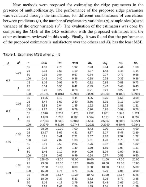
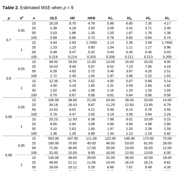
Tables 1 and 2 present the output of the simulation concerning properties of the different methods that used to choose the ridge parameter k.
Results show that the estimated MSE is affected by all factors that were varied. It is also noted that the higher the degree of correlation the higher estimated MSE, but this increase is much greater for the OLS than the ridge regression estimator. The sample size and the number of explanatory variables having a different impact of the estimators.
In Tables 1 and 2 when ρ = 0.7 and n is large, note that the estimated MSE
decreases substantially and the performance of KIs is much better than the other
ridge estimators from the MSE point of view. Finally, the OLS estimator is defeated by all of estimators.
Conclusion
Ridge regression is one of the more popular estimation procedures for addressing issues of multicollinearity. The procedures discussed herein fall into the category of biased estimation techniques. They are based on this notion: though the OLS gives unbiased estimates and indeed enjoy the minimum variance of all linear unbiased estimators, there is no upper bound on the variance of the estimators and the presence of multicollinearity may produce large variance. Biased estimation is used to attain a substantial reduction in variance with an accompanied increase in stability of the regression coefficients. The coefficients become biased, but the reduction in variance is of greater magnitude than the bias induced in the estimators.
New methods were proposed for estimating the ridge parameters in the presence of multicollinearity. The performance of the proposed ridge parameter was evaluated through the simulation, for different combinations of correlation between predictors (ρ), the number of explanatory variables (p), sample size (n) and variance of the error variable (σ2). The evaluation of the estimators was done by
comparing the MSE of the OLS estimator with the proposed estimators and the other estimators reviewed in this study. Finally, it was found that the performance of the proposed estimators is satisfactory over the others and KIs has the least MSE.
Table 1. Estimated MSE when p = 5
ρ σ2 n OLS HK HKB KI a KIg KIh KIs 0.7 0.05 15 4.53 2.75 1.92 2.23 2.34 2.44 1.68 25 2.13 1.63 1.19 1.37 1.43 1.48 1.14 50 0.95 0.84 0.67 0.74 0.77 0.79 0.68 100 0.42 0.40 0.36 0.38 0.38 0.39 0.36 1 15 1.16 0.95 0.73 0.82 0.85 0.88 0.73 25 0.54 0.50 0.42 0.45 0.47 0.48 0.43 50 0.23 0.22 0.20 0.21 0.21 0.22 0.21 100 0.1025 0.1013 0.0981 0.0995 0.1009 0.1001 0.0991 0.9 0.05 15 14.06 6.13 4.44 4.95 5.25 5.56 3.08 25 6.44 3.62 2.40 2.86 3.01 3.17 1.90 50 2.83 2.04 1.35 1.62 1.72 1.81 1.21 100 1.27 1.08 0.79 0.90 0.95 0.99 0.78 1 15 3.510 2.209 1.475 1.752 1.851 1.948 1.321 25 1.633 1.293 0.908 1.064 1.121 1.174 0.892 50 0.7063 0.6391 0.5068 0.5643 0.5867 0.6061 0.5224 100 0.3279 0.3130 0.2744 0.2921 0.2990 0.3046 0.2841 0.95 0.05 15 28.00 10.00 7.00 8.43 9.00 10.00 4.00 25 13.97 6.09 4.31 4.87 5.17 5.48 2.89 50 5.91 3.41 2.21 2.67 2.82 2.97 1.72 100 2.78 2.02 1.33 1.61 1.70 1.79 1.18 1 15 6.91 3.53 2.34 2.76 2.92 3.09 1.82 25 3.38 2.26 1.49 1.79 1.89 1.99 1.31 50 1.46 1.19 0.84 0.99 1.04 1.09 0.83 100 0.68 0.62 0.49 0.54 0.57 0.59 0.50 0.99 0.05 15 156.00 49.00 38.00 36.00 41.00 47.00 20.00 25 73.00 23.00 18.26 18.08 20.00 22.00 10.00 50 32.00 12.00 8.00 9.00 10.00 11.00 5.00 100 15.00 6.76 4.71 5.35 5.70 6.06 3.08 1 15 39.00 14.17 10.35 10.73 11.90 13.17 6.25 25 18.00 7.37 5.33 5.82 6.26 6.72 3.35 50 8.16 4.17 2.79 3.29 3.48 3.67 2.01 100 3.78 2.43 1.56 1.89 2.01 2.11 1.29
RIDGE REGRESSION AND ILL-CONDITIONING
Table 2. Estimated MSE when p = 9
ρ σ2 n OLS HK HKB KI a KIg KIh KIs 0.7 0.05 15 16.29 8.70 4.76 5.98 6.65 7.35 4.17 25 5.38 4.18 2.50 3.09 3.41 3.71 2.40 50 2.03 1.86 1.35 1.55 1.67 1.76 1.38 100 0.89 0.86 0.73 0.78 0.82 0.84 0.74 1 15 4.04 2.93 1.7483 2.13 2.35 2.58 1.7482 25 1.33 1.23 0.93 1.04 1.11 1.17 0.96 50 0.48 0.47 0.42 0.44 0.45 0.46 0.43 100 0.216 0.214 0.203 0.208 0.211 0.213 0.206 0.9 0.05 15 48.00 19.00 11.00 13.00 15.00 16.00 8.00 25 16.63 9.46 5.07 6.52 7.23 7.95 4.19 50 6.28 4.83 2.72 3.46 3.87 4.25 2.51 100 2.72 2.40 1.55 1.87 2.06 2.22 1.53 1 15 12.36 6.74 3.52 4.50 5.07 5.66 3.14 25 4.00 3.19 1.85 2.31 2.59 2.84 1.82 50 1.52 1.40 1.00 1.16 1.25 1.33 1.03 100 0.70 0.67 0.56 0.61 0.64 0.66 0.58 0.95 0.05 15 105.00 38.00 21.00 24.00 28.00 33.00 14.00 25 34.18 16.43 8.87 11.20 12.50 13.85 6.79 50 12.62 8.01 4.21 5.49 6.14 6.78 3.55 100 5.78 4.47 2.50 3.19 3.58 3.94 2.29 1 15 25.25 11.93 6.38 7.98 9.01 10.08 5.15 25 8.65 5.84 3.08 4.00 4.50 4.98 2.80 50 3.10 2.63 1.60 1.97 2.20 2.39 1.59 100 1.36 1.26 0.89 1.04 1.13 1.19 0.92 0.99 0.05 15 563.00 197.00 111.00 122.00 146.00 173.00 73.00 25 185.00 70.00 40.00 46.00 53.00 61.00 26.00 50 71.00 30.00 17.00 20.00 23.00 26.00 12.00 100 31.00 15.00 8.00 10.00 12.00 13.00 6.00 1 15 140.00 48.00 28.00 31.00 36.00 42.00 18.00 25 48.95 21.11 11.95 14.40 16.24 18.15 8.62 50 18.09 10.11 5.29 6.86 7.67 8.48 4.30 100 7.96 5.49 2.93 3.82 4.32 4.80 2.62
References
Alkhamisi, M., & Shukur, G. (2008). Developing ridge parameters for SUR model. Communications in Statistics, Theory and Methods, 37, 544-564.
Dorugade, A. V., & Kashid, D. N. (2010). Alternative method for choosing ridge parameter for regression. International Journal of Applied Mathematical Sciences, 4(9), 447-456.
Gibbons, D. G. (1981). A simulation study of some ridge estimators. Journal of the American Statistical Association, 76(373), 131-139.
Hoerl, A. E., & Kennard, R. W. (1970). Ridge Regression: Biased Estimation for non-orthogonal Problems. Technometrics, 12, 55-67.
Hoerl, A. E., & Kennard, R. W. (1976). Ridge Regression: Iterative Estimation of the biasing Parameter. Communications in Statistics, 5, 77-88.
Hoerl, A. E., Kennard, R. W., & Baldwin, K. F. (1975). Ridge Regression: some Simulation. Communications in Statistics - Theory and Methods, 4, 105-124.
Khalaf, G. (2011). Ridge Regression: An Evaluation to some New Modifications. International Journal of Statistics and Analysis, 1(4), 325-342.
Khalaf, G. (2013). A Comparison Between Biased and Unbiased Estimators. Journal of Modern Applied Statistical Methods, 12(2), 293-303. Retrieved from
http://digitalcommons.wayne.edu/jmasm/vol12/iss2/17/
Khalaf, G., & Shukur, G. (2005). Choosing Ridge Parameters for
Regression Problems. Communication in Statistics – Theory and Methods, 34, 1177-1182.
Kibria, B. M. G. (2003). Performance of some New Ridge Regression Estimators. Communication in Statistics - Theory and Methods, 32, 419-435.
Lawless, J. P., & Wang, P. A. (1976). A Simulation Study of Ridge and Other Regression Estimators. Communications in Statistics, 5, 307-323.
Saleh, A. K., & Kibria, B. M. (1993). Performances of some new
preliminary test ridge regression estimators and their properties. Communications in Statistics - Theory and Methods, 22, 2747-2764.
Troskie, C. G., & Chalton, D. O. (1996). A Bayesian estimate for the constants in ridge regression. South African Statistical Journal, 30, 119-137.