Worksite data analysis using cloud services for machine learning

(1)

WORKSITE DATA ANALYSIS USING

CLOUD SERVICES FOR MACHINE

LEARNING

Faculty of Information Technology and Communication Sciences Master’s thesis October 2019

(2)

ABSTRACT

Samu Jussila: Worksite data analysis using cloud services for machine learning Master’s thesis

Tampere University Software Engineering October 2019

This thesis studies utilizing machine learning in cloud services. The aim of the thesis was to create a machine learning pipeline in a cloud service platform and use the pipeline to test how well worksite data could be used for machine learning. The data was operational data already existing in a database, and the test done was predicting a worksite’s time of completion based on its state and history using different machine learning models.

The pipeline was built in Amazon Web Services, and consisted mainly of the services Glue and SageMaker. Glue was used to transform the data into a format readable by machine learning models, and SageMaker was used to implement the machine learning models. Amazon Web Services had a ways of creating all the needed parts of the pipeline, and the amount of boilerplate code was minimal. The implementation was sufficiently easy with no large setbacks.

The machine learning models implemented were linear regression, random forest, XGBoost, and artificial neural network. The model performance results show that the best model for this problem is a two-hidden-layer artificial neural network, but the results vary drastically by the method the whole data set is split into training and test data.

Keywords: Machine learning, cloud services, Amazon Web Services, regression, comparison, pipeline

(3)

TIIVISTELMÄ

Samu Jussila: Työmaadatan analysointi käyttäen pilvipalvelun tarjoamaa koneoppimista Diplomityö

Tampereen yliopisto Ohjelmistotuotanto Lokakuu 2019

Tässä työssä tutkitaan koneoppimispalvelujen käyttöä pilvipalvelualustalla. Työn tavoitteena oli rakentaa pilvipalvelualustalle dataputki, jolla voidaan rakentaa käyttökelpoisia koneoppimis-malleja käyttäen operationaalista työmaadataa olemassaolevasta tietokannasta. Datan soveltu-vuutta koneoppimistarkoituksiin mitattiin ennustamalla työmaan valmistumisaikaa sen nykytilan ja historian perusteella käyttäen erilaisia koneoppimismalleja.

Dataputki rakennettiin Amazon Web Services -pilvipalvelussa, ja koostui pääosin Glue- ja SageMaker-palveluista. Glue:a käytettiin operationaalisen datan muuntamiseen koneoppimismal-lien lukemaan muotoon, ja SageMaker:ia rakentamaan mallit. Amazon Web Services -alusta sisäl-si tarvittavat palvelut putken rakentamiseen, eikä ylimääräistä itse putkeen liittyvä koodia tarvinnut kirjoittaa juurikaan. Putki oli helppo toteuttaa, eikä suuria vaikeuksia tullut vastaan.

Koneoppimismallit, joilla dataa testattiin olivat lineaarinen regressio, random forest, XGBoost sekä neuroverkko. Tulokset näyttävät, että paras malli tähän ongelmaan on kahden piilotetun ker-roksen neuroverkko, mutta tarkkuuteen vaikuttaa huomattavasti tapa, jolla koko data puolitetaan opetus- ja testidataan.

Avainsanat: Koneoppiminen, pilvipalvelut, Amazon Web Services, regressio, vertailu, dataputki Tämän julkaisun alkuperäisyys on tarkastettu Turnitin OriginalityCheck -ohjelmalla.

(4)

PREFACE

This thesis was written in Tampere, Finland between February and October 2019. I learned a lot while writing this thesis, and would like to thank my colleague Hannu Hytö-nen for providing me with this interesting topic, and my employer Bitwise Oy for granting the time to work on it. I would also like to thank Professor Hannu-Matti Järvinen and As-sociate Professor Heikki Huttunen for supervising this work and giving detailed feedback on it. Lastly, thanks go to Inari for providing insights into scientific writing and supporting me.

Tampere, 2nd October 2019 Samu Jussila

(5)

LIST OF SYMBOLS AND ABBREVIATIONS

ANN Artificial Neural Network AWS Amazon Web Services

CART Classification And Regression Tree CSV Comma-separated Values

Epoch An iteration of all the training data passing through an artificial neu-ral network

HTTP Hypertext Transfer Protocol. The underlying protocol of communi-cations through the Internet

Loss An artificial neural network’s error function to minimize MAE Mean Absolute Error

MLP Multilayer Perceptron MSE Mean Squared Error

S3 Simple Storage Service. The object storage service in Amazon Web Services

SGD Stochastic Gradient Descent

SQL Structured Query Language. A common way of accessing data in a database.

SSH Secure Shell. A protocol for secure remote access UI User interface

URL Uniform resource locator XGBoost eXtreme Gradient Boosting

(8)

1 INTRODUCTION

Machine learning is a popular topic in the field of technology, and is being utilized by com-panies for an ever increasing amount of tasks which would previously require a human, or an inferior hard-coded solution. Machine learning solutions can be used to for exam-ple to identify tumors in brain images [43], detect malicious users in computer networks [40], play the game of go better than humans [39], and predicting the durations of traffic incidents [45]. A correctly functioning machine learning application requires a lot of data, and many companies have proactively gathered data and are looking for ways to utilize it with machine learning.

Cloud services are a relatively recent alternative to on-premise hosting of services. Cloud services free their users of the burdens of managing physical infrastructure. In the cloud, infrastructure can be easily scaled up or down based on demand, even automatically, and the information can be accessed from anywhere in the internet [20]. An increasing number of companies are starting to utilize cloud services [35]. Cloud service providers have also started offering machine learning services on their cloud platforms. Other applications and the data needed for a machine learning process might already be stored in the cloud platform, which makes starting utilizing machine learning easier. Difficult machine learning tasks also require powerful hardware, which are easily accessible in the cloud.

This thesis aims to perform data analysis on existing operational data in a cloud service database, using machine learning. The goal is to first choose a cloud service platform, and then study how the data applies to a meaningful machine learning task, and how well the platform supports building a usable application utilizing the machine learning results. The machine learning task for this thesis has been chosen to be predicting a worksite’s time of completion, using its state and history as input.

The goals are met using the design science methodology [19]. In this work, a proof-of-concept application is designed, consisting of two artifacts constructed using cloud services. The first artifact is a data pipeline from an operational database to using the machine learning results. The second artifact are the machine learning models. The pipeline’s performance is evaluated based on its ease of construction and its functionality for actual use. The machine learning models are all evaluated with well-known popular accuracy metrics, and the best one is chosen for possible future use.

(9)

will be presented, and then the mathematical background of each model used will be explained in more detail. Chapter 3 will give a more detailed explanation of what the cloud is, and what kind of services are offered in the cloud. How machine learning services are implemented in the cloud is also discussed. Chapter 4 will first explain the choice of the cloud platform used. Then the architecture for the machine learning applications is presented. The results of both utility of the data, and the suitability of the cloud platform, will be presented and discussed in Chapter 5. Finally, in Chapter 6, the results are briefly summed up.

(10)

2 MACHINE LEARNING

Machine learning is a field of research which studies computer programs that automati-cally learn from examples [30]. There are numerous different domains and applications where machine learning is used, including analysing images for medical purposes, secu-rity heuristics for protecting ports of networks, object recognition for self-driving cars and pattern recognition for detecting weaknesses in code [25].

Machine learning in general uses the principle ofConcept learning: learning broad con-cepts through sets of specific examples [30]. What this means is that a computer is taught to perform the wanted task by giving it examples of how it should work, and hop-ing it learns the actual concept which the examples try to illustrate. Once the computer is taught the principles through the examples, later called training data, it can use its acquired knowledge to correctly perform even with data outside of the set of examples it learned with. For example, a simple image recognition task could have the computer learn to recognize whether there is a cat or a dog in an image. The computer is shown images with either a cat or a dog in them, and told what it should output. Eventually, after having seen enough images, the computer should learn to correctly identify the animal in any image it is shown, even ones it has not been shown before and told the right answer to.

Machine learning applications are implemented using mathematical constructs, called

models. A trained model is the output of a machine learning algorithm using the provided training data [14]. The model can be used to infer the trained attributes from new data. A model’s performance depends on both the structure of the model itself, and the amount and quality of the training data. Some of the most common reasons for models performing poorly areover-fitting,under-fitting [14].

Over-fitting means the model performs excellently with the examples it was trained with, but poorly with any data it was not trained with. Over-fitting can occur when the model is too complex to represent the principle it is trying to learn, or when there is not enough training data to model the principle in enough detail [2]. An over-fit model in effect, or even literally, just memorizes the training data and does not learn the correct principle [14]. Generally, to overcome over-fitting, either the model complexity has to be reduced, or the amount of training data has to be increased [2]. Under-fitting is the opposite of over-fitting [14]. Under-fitting can happen if the model is not complex enough to represent the taught principle, and gives poor results. Under-fitting can be overcome by increasing model complexity to match the complexity of the learned principle.

(11)

This chapter will first further describe types of machine learning problems. Secondly, the machine learning models used in this thesis will be discussed in more detail.

2.1 Types of machine learning

Machine learning algorithms can be roughly split into three categories: supervised learn-ing, unsupervised learning and reinforcement learning [42]. Supervised learning means teaching the computer to mimic the training data. Training data in supervised learning consists of pairs of inputs and desired outputs. Theis there a cat or a dog in the image

problem described earlier is a supervised learning problem, where the input is an image, and the output is the boolean value "yes" or "no" corresponding to the image. [25]. The previous example is a classification problem. Classification means training the com-puter to choose the most probably correct one of predefined labels, classes, for each input data. The other sub category of supervised learning is regression. A regression problem means training the computer to infer or predict a continuous value from the input data. An example of a regression task would be predicting salary of a job based on its description. [17]

Unsupervised learning algorithms, unlike supervised learning, do not try to output a value based on input values, as there are no known output values for the input data to train the model with. Instead unsupervised learning algorithms perform analysis on and recognize patterns in the data itself [13]. Some examples of usages for unsupervised learning algo-rithms are clustering, dimensionality reduction [25] and anomaly detection [16]. Cluster-ing algorithms divide the data into categories inferred by the algorithms themselves [25]. Dimensionality reduction algorithms take high-dimensional data sets, and transform them into fewer dimensions, trying to take only the most valuable features into the reduced set [25]. Anomaly detection algorithms look for anomalies or outliers in data, for example to detect credit card frauds or a system breakdown [6].

Reinforcement learning is training a computer to choose a correct action in its observable environment state. In reinforcement learning the computer has to find which action ulti-mately yields the largest numerical reward [42]. The reward may not be immediate, which makes reinforcement learning different from supervised learning: In supervised learning the training data would include correct actions for the data set’s environment states, but in reinforcement learning, they are not known, and the only thing which matters is the final reward. The computer has to then, by trial-and-error, find a policy which leads to the best outcome from any environment state.

A well-known example of a reinforcement learning algorithm is AlphaGo, the program which has won some of the world’s best human players in go [39]. A reinforcement learning algorithm learning to play go could be given a positive reward for winning a game, and a negative reward for losing a game. The ultimate reward then reinforces or diminishes the choices the algorithm made during the game.

(12)

2.2 Models

The data used in this thesis has known output values for the training data, and the output values are continuous numbers, which means that the algorithms used in the thesis be-long to supervised learning and regression. This section introduces the machine learning models used in the thesis.

2.2.1 Linear regression

This section will explain the mathematical background used in linear regression models for machine learning.

Simple linear regression

Simple linear regression is a model which has a single input variablex, and a response y. The model represents a straight line, and can be represented as

y =β0+β1x+ϵ (2.1)

whereβ0andβ1are unknown constants, usually also called regression coefficients. They

denote slope and intercept respectively. ϵis a random error component. The errors are assumed to be uncorrelated random variables with zero mean and variance σ2_{. The}

resultycan be seen as a probability distribution with mean

E(y|x) =β0+β1x (2.2)

and variance

V ar(y|x) =σ2 (2.3)

as the mean of the error is zero, and the unknowns are constants with no error. [31] The regression coefficients can be estimated from training data ((x1, y1), (x2, y2), ...,

(xn, yn)) using the method of least squares, which finds values with which the sum of squared residuals, differences between the wanted output and the model output, is the smallest. Givenβˆ0andβˆ1, which estimateβ0andβ1, difference between the training data

yi and the model outputyˆi for inputxi is

(13)

The squared sum of residuals,RSS(β0, β1)is then RSS(β0, β1) = n ∑ i=1 (yi−(β0+β1xi))2. (2.5)

The minimum can be found by partially differentiating the sum function with respect to both β0 and β1, setting the derivatives equal to 0, and solving the equation pair. This

ultimately yields ˆ β1 = ∑n i=1((xi−x)(yi−y)) ∑n i=1(xi−x)2 (2.6) and ˆ β0 =y−βˆ1x (2.7)

wherexandyare the averages [31],[46] x= 1 n n ∑ i=1 xi, y= 1 n n ∑ i=1 yi. (2.8)

Multiple linear regression

Simple linear regression can only have one dimension in its input variablexi, which does not fulfill the general case, where there can be any number of dimensions. The equations of 2.2.1 can however be extended to consider any number of dimensions.

The multiple linear regression model withkinput dimensions is defined as

yi=β0+β1xi,1+β2xi,2+...+βkxi,k+ϵ (2.9)

whereβ1..k are the regression coefficients, xn,1..k are the input values,y the response, andϵthe random residual. [31],[46]

The regression coefficients can, similar to 2.2.1, be estimated using the method of least squares. Given training data (n sets of parameters and results: (x1,1, x1,2, ..., x1,k, y1),

(x2,1, x2,2, ..., x2,k, y2), (xn,1, xn,2, ..., xn,k, yn)), and parametersβˆ0,βˆ1,βˆ2, ...,βˆk, theith re-sponseyˆi by the model is [31],[46]

ˆ

yi= ˆβ0+ ˆβ1xi,1+ ˆβ2xi,2+...+ ˆβkxi,k +ϵi. (2.10) Least squares method minimises the sum of squared residuals, which can be written analogous to 2.5 as [31],[46] RSS(β0, β1, β2, ..., βk) = n ∑ i=1 ϵ2_i = n ∑ i=1 (yi−yˆi)2= n ∑ i=1 (yi−βˆ0− k ∑ j=1 ( ˆβjxi,j))2. (2.11)

(14)

Minimising the sum can be done by differentiating with respect to eachβj, j = 1..k, setting the derivative to zero, and solving the system of equations. [31],[46]

Equation 2.11 can be conveniently expressed in matrix notation as [31],[46] RSS(β) = n ∑ i=1 ϵTϵ= (y−Xβ)T(y−Xβ) (2.12) where y= ⎡ ⎢ ⎢ ⎢ ⎢ ⎢ ⎢ ⎣ y1 y2 .. . yn ⎤ ⎥ ⎥ ⎥ ⎥ ⎥ ⎥ ⎦ ,X = ⎡ ⎢ ⎢ ⎢ ⎢ ⎢ ⎢ ⎣ 1 x1,1 x1,2 . . . x1,k 1 x2,1 x2,2 . . . x2,k .. . ... ... . .. ... 1 xn,1 xn,2 . . . xn,k ⎤ ⎥ ⎥ ⎥ ⎥ ⎥ ⎥ ⎦ ,β= ⎡ ⎢ ⎢ ⎢ ⎢ ⎢ ⎢ ⎢ ⎢ ⎢ ⎢ ⎣ β0 β1 β2 .. . βk ⎤ ⎥ ⎥ ⎥ ⎥ ⎥ ⎥ ⎥ ⎥ ⎥ ⎥ ⎦ ,ϵ= ⎡ ⎢ ⎢ ⎢ ⎢ ⎢ ⎢ ⎣ ϵ1 ϵ2 .. . ϵk ⎤ ⎥ ⎥ ⎥ ⎥ ⎥ ⎥ ⎦ . (2.13)

From equation 2.12, the estimateβˆcan be solved as [18, p. 45] ˆ

β= (XTX)−1XTy, (2.14) provided that the inverse (XTX)−1 exists. The inverse will exist if the regressors are linearly independent.

The estimator only depends on the statisticsXTX andXTy, which are the uncorrected sums of squares and cross products between the columns ofX, and uncorrected sums of cross products between columns of X and y. [31],[46] The least squares estimate

ˆ

β should not be calculated using 2.14, because the uncorrected sums are susceptible to large rounding errors, which may make the result inaccurate. Instead the calculations should be done on corrected sums instead. [46] The matrix U is defined as the train-ing data parameters matrix X without the first column of ones, and the column means subtracted from each column

U = ⎡ ⎢ ⎢ ⎢ ⎢ ⎢ ⎢ ⎣ (x1,1−x1) . . . (x1,k−xk) (x2,1−x1) . . . (x2,k−xk) .. . . .. ... (xn,1−x1) . . . (xn,k−xk) ⎤ ⎥ ⎥ ⎥ ⎥ ⎥ ⎥ ⎦ (2.15)

(15)

ysubtracted from each element V = ⎡ ⎢ ⎢ ⎢ ⎢ ⎢ ⎢ ⎣ y1−y y2−y .. . yn−y ⎤ ⎥ ⎥ ⎥ ⎥ ⎥ ⎥ ⎦ . (2.16)

The matricesUTU andUTV have the same needed statistical properties as the matrices XTX andXTy, and can be used to calculate βˆmore accurately, very similarly to 2.14 as

ˆ

β∗ = (UTU)−1UTV, βˆ0 =y−βˆ∗

T

x (2.17)

whereβˆ∗is the vector containing all values ofβˆexcept for the intercept,βˆ0. [46]

The vector βˆ can be used to predict an unknown value yˆ_u by multiplying a parameter vectorxT ([1,xu,1,xu,2,...,xu,k]) with it:

ˆ y=xTβˆ= ˆβ0+ k ∑ j=1 ˆ βjxj (2.18)

or multiple predictions at once by [31],[46] ˆ

y=Xβˆ. (2.19)

2.2.2 Decision trees ensembles

Decision tree learning is a machine learning algorithm which constructs a decision tree to learn the wanted principle from training data. Decision trees can be used as a model alone, but multiple trees can also be aggregated as a single ensemble, a forest. The two most popular ensemble methods for decision trees are randomization andboosting. This section will first explain decision trees themselves, and present an algorithm for creating them. Then, the algorithms used to create the ensemble models used in this thesis are explained.

Decision trees

A decision tree is a model which consists of a root node, intermediate nodes, and leaf nodes. Each node contains either a test on one of the parameters of the input data, or the final answer (a leaf node). When using a decision tree to find the output value from input data, the root node is accessed first. By following the branches of the tree by

(16)

Figure 2.1.Decision tree for inferring monthly rent based on apartment location, amount of rooms, and whether the apartment is shared with others

answering the tests in the nodes with the input data eventually a leaf node containing the final value is reached. [30] For example, a simple decision tree in Figure 2.1 could be used to give an estimate on apartment’s monthly rent using three parameters as input data. The parameters in this case would be a boolean value of whether the apartment is located in the center of the city, a number of how many rooms there are in the apartment, and a boolean value of whether the apartment is shared with other people. The leaf nodes give an estimate based on the answers given to get to that leaf.

Decision tree learning is an efficient and simple learning model, especially so with large amounts of dimensions and training data. They are trained with greedy divide-and-conquer algorithms, which recursively split the data into smaller and smaller subsets. [44] There are many specific algorithms for constructing a decision tree, such as ID3, ASSISTANT, C4.5 [30] and CART [48]. The CART algorithm will be explained in detail, as very similar algorithms to it are used by both the random forest algorithm [4] and the XGBoost algorithm [33, p. 50], which are the tree ensemble methods used in this thesis. In regression problems decision tree models’ weaknesses include instability [44], non-smoothness [44][2, p. 666], many algorithms only doing a split on one variable in a

(17)

node [2, p. 666]. A decision tree is unstable, because each node splits the data, and the following branches only have part of the data to use, and depend on their parent nodes’ decisions. If there are two training data sets with only minimal differences, tree models trained from them could have completely different structures, if the root node’s decision parameter changes even a little. Non-smoothness is problem only in regression models. It means that the tree can only give a finite amount of discrete final answers for any parameters, as a leaf node only contains one value. Typically regression models are trying to model smooth functions instead of a choice out of discrete values [2, p. 666]. Doing a split on only one variable can lead to much more complex trees than would be needed if many variables were considered. For example, if a decision boundary between two values could be easily expressed as the sum of two variables, single variable splitting cannot represent that in a simple way. A sum of two variables requires a decision boundary diagonal to both variable axes. Instead a single variable splitting tree model uses numerous splits of both variables to emulate the diagonal line. [2, p. 666] Decision trees also very susceptible to over-fitting if they are not sufficiently constrained [44].

CART algorithm

The CART algorithm, introduced by Breiman et al. in 1984, produces binary trees which split the data in two by one variable in each node. The algorithm provides tools for creating both classification and regression trees, but this explanation only focuses on regression. CART trees are also capable of using both least squares and the least absolute deviation as error measures, but this explanation will only focus on the least squares method. The algorithm consists of the following steps [48]:

1. Grow a large tree

2. Iteratively prune the tree back to its root 3. Choose the best tree acquired during pruning

The first step is growing a large treeTmax. This is done by recursively splitting the training data in nodes until a stopping condition in each branch is satisfied and the leaf nodes are grown. The recursive split is done by choosing the best split from the set of possible splits on any one variable. The variables can be either categorical or numerical. A split on a numerical value xn in CART is always of the form xn ≤ A, where A is a constant number. A split on a categorical variablexnis of the formxn∈B whereB is a subset of all possible values ofxn. [3]

The best split for a regression tree in CART is defined as the split which most decreases error measureR(t), where tis the node in question. The best splits∗out of all possible splitsS is defined as

∆R(s∗, t) = max

s∈S ∆R(s, t), (2.20)

where

(18)

The variables tL andtR are the left and right branches of the node as the result of the splits.

Define xnas the nth training data instance in node t,N as the number of training data instances in nodet,ynas thenth response,y(t)as the average of all the response values in nodet, andp(t)as the proportion of training data instances in nodet(N(t)/Ntotal). The R(t)itself can be then defined as

R(t) =s2(t)p(t) (2.22) where s2(t) = 1 N ∑ xn∈t (yn−y(t))2. (2.23)

It is worth noting that s2(t) is the sample variance of the response variables in nodet, and the best split is then the one which reduces the weighted sum of variances the most. The splitting is done in each node until a stopping condition is met. CART trees are grown deliberately large, so the only stopping rule usually used isN(t) ≤Nmin, whereNmin is usually 5 [3, p. 233]. Other possible stopping rules include the tree’s maximum depth limit, and all the response variables being exactly the same. When a stopping condition is met, the node becomes a leaf node, and it is assigned a single response value. The response valuey(t)for nodetis

y(t) = 1

N(t)

∑

xn∈t

yn, (2.24)

which is the arithmetic average of the response variables of training data in the node. [3] Least squares regression error for modelβin general is defined as [44, p. 63]

Err(β) = 1 N N ∑ n=1 (yn−r(β,xn))2, (2.25)

wherer(β,xn)is the response value given by the model for the input data. A tree model’s total errorErr(T)is defined as the weighted average of its leaves’ errors [44]

Err(T) =∑

l∈T˜

p(l)Err(l), (2.26)

and a leaf node’s error as the mean squared error in that node Err(l) = 1

Nl ∑

xn∈l

(yn−yl)2. (2.27)

A CART tree minimizesR(t)of its leaf nodes, which is the weighted least squared error criterion. Thus, a CART tree minimizes least squares error criterion.

(19)

The second step in CART algorithm is pruning the tree back to its root. Pruning means picking a node, and deleting all its descendant nodes, aggregating all the training data in its descendants to itself. The algorithm uses pruning instead of more elaborate stopping conditions, because no stopping rule gives generally as good results as pruning post-growing does [3, p. 61-62]. Pruning a large tree Tmax back to its root means pruning the tree until only its root exists. During the process each intermediate step of pruning is saved, and a sequence of treesTmax→T1→T2→ · · · →Troot is acquired.

The sequence of pruned trees is acquired through complexity pruning. In error-complexity pruning the tree is assigned an error-error-complexity measureRα(T), which is the linear combination of the error measureR(T) =Err(T)and the amount of leaf nodes in the tree|T˜|

Rα(T) =R(T) +α|T˜|. (2.28) For each value of the cost complexityα there is a subtree Tα which minimizes Rα(Tα). By increasingα, different minimizing subtrees of the sequence are found, and eventually the cost for having any number of leaf nodes at all is so large that the minimizing tree is just the root node.

In practice this is done in reverse, by cutting weakest links in the trees, and finding the corresponding α values. Define {t} as nodet made into a leaf node by deleting all its descendants, andTtas the subtree starting from nodet. Now, for each node

Rα({t}) =R(t) +α, (2.29) and

Rα(Tt) =R(Tt) +α|T˜_t|, (2.30) where R(Tt) = Err(Tt), the weighted sum of the leaf nodes below Tt. As long as Rα(Tt) < Rα({t}), the complexity of the branch is acceptable to lower the error mea-sure, but for every node t, there is some value of α, where deleting the descendants starts producing lower overall error-complexity. For every node, the valueg(t), the lowest αwhere the nodes’s descendants are pruned can be calculated as

g(t) = ⎧ ⎨ ⎩ R({t})−R(Tt) |T˜t|−1 , ift / ∈T˜ ∞, ift∈T˜ . (2.31)

Weakest link is the nodetwhere

g(t) = min

t∈T g(t). (2.32)

The weakest link is cut, and the next tree in the pruning sequence is acquired. [3]

The final step in CART is to choose the best tree in the pruning sequence. This is done by using either cross validation or test set. In test set method, some number of training data

(20)

is taken out of the data set and not used to construct the tree. Then the taken-out test set is used to assess the accuracy of each tree in the pruning sequence and the best tree size is picked. Cross validation makesvdifferent pruning sequences where eachTv,max is grown with v−_v1N training data samples and tested with the remaining 1_vN. When vis large, each sequence’s trees’ accuracy is very similar to the trees grown with all the data, and cross validation gives a good estimate of the right size of a tree. [3]

Random forest

Random forest is a machine learning model, which consists of an ensemble of individual trees. Random forests grow the individual trees using bootstrap aggregation (bagging). Using bagging, each individual tree is trained with a randomly selected subsetXnof the whole training dataX. The selection is made by taking a random sample from the training data with replacement, and a random sample from the dimensions without replacement. The individual trees are then grown with the CART algorithm, but modified in two ways: The trees are not pruned, and the best split at each node is found in a small random subset of features instead of all the features. Finally, when making predictions with new data, the whole regression model’s output F(X) for input parameters is the average of the set of all the individual trees’ predictions{Tk(X)}[4]

F(X) = 1 K K ∑ k=1 Tk(X). (2.33)

The random forest method improves on single trees by creating multiple strong predictors, which do not under-fit, but do over-fit severely. The effect of over-fitting is lessened by having the individual trees be independent of each other, and the result is, in theory, a model which does not under-fit and over-fits very little. As the number of trees in the forest grows towards infinity, the mean squared error of the forest approaches a limit, and makes the error of the forestF

P E∗(F)≤ρP E∗(T), (2.34) whereP E∗(T) is the average error of a single tree in the forest, andρ is the weighted correlation between the errors of the individual trees. This shows that in order for a random forest to be any better than a single tree, the randomization has to aim to as independent subsets of the data and the input variables as possible. [4]

Random forests are very resistant to noise because of the averaging effect of the ensem-ble. Random forests deal with the weaknesses of single decision trees too. They have much smoother result variables, as their output does not have to be a single value from the training set. Instability is not a property of random forests, as they are averages of many unstable trees. Random forests are very fast to generate compared to their size, as all the individual trees being independent of each other, they can be constructed in

(21)

parallel.

Gradient Boosting

Boosting models create ensembles consisting of multiple single models, but the approach is very different from randomization. Boosting models instead add new, weak single mod-els, later referred to as base learners, to the ensemble sequentially and incrementally. The new base learner added is trained to correct the errors of the whole ensemble. [32] Boosting uses weak base learners to battle the over-fitting and under-fitting dilemma. The idea is reverse from the randomization method used by random forests. A weak leaner does not over-fit at all, but under-fits the data severely. New models are sequentially added to correct the errors, which can only be due to under-fitting. When adding new base learners, under-fitting is decreased, while over-fitting increases only a little.

Gradient boosting algorithms minimize the expected value of some loss functionL(y, F(x)), which can be for example the squared error between the real output valuey and the out-put given by the modelF(x). The modelF is a weighted sum ofK weak base learners ϕ(x) F(x) = K ∑ k=0 βkϕk(x), (2.35)

and is constructed by first taking some initial guessF0(x), which is just a constant value

minimizing the loss function most as

F0(x) = arg min ρ N ∑ i=1 L(yi, ρ). (2.36)

Then, each next addition, orboost to the ensemble is calculated as the function which most decreases the loss function if summed with the rest of the ensemble

(βk, ϕk) = arg min β,h N ∑ i=1 L(yi, Fk−1(xi) +βϕ(xi)), (2.37) with the new model then being [11][32][10]

Fk=Fk−1+βkϕk. (2.38) As the optimal parameters (βk, ϕk) can be difficult to calculate in practice [32][10], an easier procedure is used. The procedure is to instead find the base learner most parallel to the negative gradienty˜iof the ensemble, and then find the weight for the found learner. The negative gradient is the derivative of the loss function

˜

yi=−

∂L(yi, Fk−1(xi)) ∂Fk−1(xi)

(22)

The base learnerϕk is then found by a simpler least squares minimization ϕk = arg min ρ,h N ∑ i=1 (˜yi−ρϕ(xi))2. (2.40)

The weightβkis then found using the original minimization equation 2.37 butϕkfixed, as [10][11] βk= arg min β N ∑ i=1 L(yi, Fk−1(xi) +βϕk(xi)). (2.41)

Gradient boosting with least squares error regression makes calculating the negative gradienty˜i very simple in practice. The gradient reduces to

˜

yi =yi−Fk−1(xi), (2.42) which means that using least squares as the loss function causes each boosting base learner to be fit to the literal errors of the ensemble before it. [10]

Gradient tree boosting is a case of gradient boosting, where the weak base learnerϕ(x)

is a decision tree, and in this thesis’s context, a regression CART tree. A tree’s output is just the constant value in the leaf which the input data belongs to. It can be expressed as the sum over allJ leaf nodes, but only if the input belongs to the parameter spaceRj which leads to thejth leaf

ϕ(x) = J ∑ j=1 bjI(x∈Rj), (2.43) where I(a) = ⎧ ⎨ ⎩ 1, ifa=true 0, ifa=f alse . (2.44)

A gradient tree boosting model’s equation 2.38 becomes [10]

Fk=Fk−1+ J ∑ j=1 γjkI(x∈Rjk), (2.45) where γjk = arg min γ ∑ xi∈Rjk L(yi, Fk−1(xi) +γ). (2.46)

XGBoost (eXtreme Gradient Boosting) is an algorithm which extends the basic gradient tree boosting algorithm. XGBoost tries to find the next tree by minimizing an objective functionL L= N ∑ i=1 [L(yi, Fk−1(xi)) +giϕk(xi) + 1 2hiϕ 2 k(xi)] + Ω(ϕk), (2.47) where−gi is the negative gradienty˜i from equation 2.39 andhi is the second derivative

(23)

of the loss hi = ∂2L(yi, Fk−1(xi)) ∂2_F k−1(xi) . (2.48)

Ωis a model complexity value, defined as

Ω(Fk) =γJ + 1 2λ J ∑ j=1 w_j2, (2.49)

whereJ is the number of leaves, andwj is thejth leaf node’s response value. λandγ are complexity costs for the values and number of the leaves. By removing the constant parts from the objective function, it simplifies into [8]

˜ L= N ∑ i=1 [giϕk(xi) + 1 2hiϕ 2 k(xi)] + Ω(ϕk) (2.50)

XGBoost constructs its single trees using the objective function. The optimal value for a leafjis given by w∗_j =− Gj Hj +λ , (2.51) where Gj = ∑ i∈Ij gi, Hj = ∑ i∈Ij hi, (2.52)

Ij being the set of instances in thejth leaf node. The quality of a tree structureqis given by

˜ L(q) =−1 2 J ∑ j=1 G2 H+λ+γJ, (2.53)

and the best split s∗ at each node is the one which most increases the quality of the structure, as s∗ = arg max s 1 2( G2_L HL+λ + G 2 R HR+λ + G 2 j Hj+λ )−γ, (2.54)

whereGL,GR, andHL,HRare the values in the left and right nodes in the proposed split [8]. If no gain is positive, no split is done at the node, and it will stay as a leaf node [47]. XGBoost has achieved recognition as being fast and scalable [8] as well as winning nu-merous machine learning competitions [33]. Tree boosting in general deals with some of the problems of single regression trees. Boosted models can yield smoother responses than single trees, but a boosted models are still unstable. Boosted models are slower to generate than random forests, because they depend on the previous trees and thus cannot be created in parallel. Boosted trees can also over-fit, if too many trees are grown into the sequence.

(24)

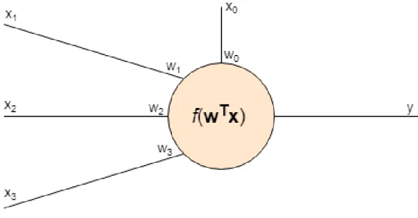
Figure 2.2. Neuron in an artificial neural network

2.2.3 Artificial neural network

Artificial neural network (ANN) is a machine learning model which comprises multiple

neuronsthat interconnect in some way. The background for artificial neural networks is in neural activity in the human brain. The neurons in a brain send electrical signals to each other with chemical rules to process information, while the neurons in artificial neural networks output numbers to other neurons to calculate a result value for input values. Although ANNs are inspired by biological neural networks, they do not aim to exactly model the networks in a human brain [30].

This thesis will only consider one neural network model, themultilayer perceptron, which is the most widely used neural network model [2]. In this section, the principles of a single neuron will be first explained, followed by constructing a multilayer perceptron out of the neurons. Finally, the mathematics of training the network with training data will be introduced.

Neuron

A neuron in an ANN consists of inputs, weights, and an activation function. The basic structure is illustrated in Figure 2.2. A neuron’s input variables can consist of raw input values or output values of other neurons. The input vectors are padded with the value1to allow neurons to add a constant value, abiasto the inputs. If there arekinput variables to the neuron, the input vectorxis then

x= [1, x1, x2, . . . , xk]T. (2.55)

(25)

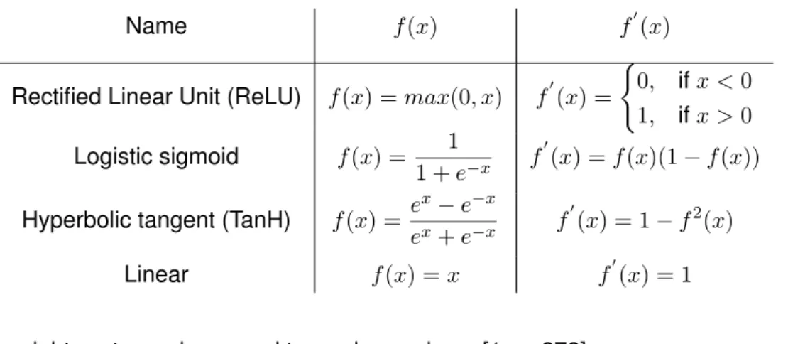
-Table 2.1. Common activation functions and their derivatives.

Name f(x) f′(x)

Rectified Linear Unit (ReLU) f(x) =max(0, x) f′(x) =

{ 0, ifx <0 1, ifx >0 Logistic sigmoid f(x) = 1 1 +e−x f ′ (x) =f(x)(1−f(x))

Hyperbolic tangent (TanH) f(x) = e

x₋_e−x

ex₊_e−x f

′

(x) = 1−f2(x)

Linear f(x) =x f′(x) = 1

length weight vector and summed to produce valuea[1, p. 272]

a=wTx. (2.56)

The valuea is very analogous to a linear regression model output described in section 2.2.1.

A neuron’s output value y is obtained by using an activation function f. An activation function has to be differentiable, as the differentials are used when training the network. The activation functions in general are also nonlinear, as if all activation functions in a network were linear, the network could be reduced to linear regression [2]. Some com-mon activation functions [23] are shown in table 2.1. Using a chosen activation function f [2],

z=f(a). (2.57)

Multilayer perceptron

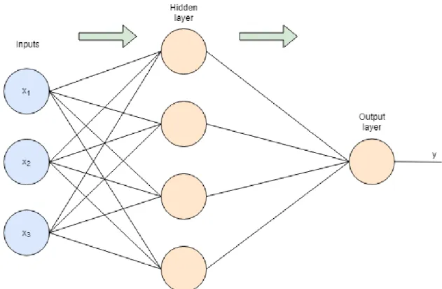
A multilayer perceptron (MLP) is a type neural network which consists of successive layers of parallel neurons. An MLP is afeed-forward network, meaning that the neurons only feed their outputs forwards, not creating any cycles in the network. This means the output of the a network is a deterministic function of only the input values.

Figure 2.3 depicts an MLP which takes three-dimensional inputs, and outputs one value. It has one hidden layer of neurons in between the inputs and outputs. The layers are all densely connected. It means that each hidden layer unit takes all three dimensions of the input layer as their inputs and the output layer neuron takes all four dimensions output by the hidden layer as its input. DefineI as the number of input dimensions, andH as the number of hidden layers. With the activation function of the output layer σ and the activation functions in the hidden layerh, the output of the network can be expressed as [2] y =σ( H ∑ j=0 w_j(2)h( I ∑ i=0 w_ji(1)xi)). (2.58)

(26)

Figure 2.3. A multilayer perceptron with three input dimensions, four hidden neurons, and one output value

The superscripts denote the layer of the neuron containing the weight.

Gradient descent

The topology of an MLP does not change once it is constructed. Thus the only thing to change in the network structure are the weights inside the neurons. The weights are updated using a weight adjustment algorithm, which uses the gradients of the errors of output values as inputs. The error gradients at each neuron are acquired through the

backpropagationalgorithm explained later in this section. [2]

The traditionally most popular weight adjustment algorithm isstochastic gradient descent

(SGD), which is an approximation of the gradient descent algorithm. The gradient de-scent algorithm is a simple formula to update the weight vectorwof a neuron. Denoting superscript(τ)as the current weights and(τ + 1)as the new weights, gradient descent rule is

w(τ+1) =w(τ)−η∇E(w(τ)), (2.59) where∇E(w) is the sum gradient of all the training data rows’ errors, andη is learning rate constant. Learning rate is a small number which denotes how fast the weights move towards the gradient. The normal gradient descent can be very slow in practice [30, p. 92][24], and the stochastic approximation is usually used instead. SGD instead updates

(27)

weights one training data sample at a time [2]

w(τ+1) =w(τ)−η∇En(w(τ)). (2.60)

SGD, while faster than normal gradient descent, can still be quite slow to converge [36][24], and many variations and extensions of it have been created. Momentum is a technique which makes the weights accelerate towards the negative gradient if the gra-dient direction stays same. Each weight has its own momentum, and the momentum instead of the weight is updated towards the gradient

v(τ+1) =γv(τ)+η∇E(w(τ))

w(τ+1)=w(τ)−v(τ+1).

(2.61)

The variable γ is a decay term, which gradually slows the speed of change. Another variation to SGD is adjusting learning rate dynamically. TheAdagradalgorithm does this by dividing the learning rate at each iteration and weight by the square root ofG(_i,iτ), where Gis a diagonal matrix containing the sum of the squares of each of the neurons’s weights gradients up to timeτ. The formula is

wi(τ+1) =wi(τ)− η √

G(_i,iτ)+ϵ

∇En(wi(τ)), (2.62)

whereϵis a small positive constant to avoid division by zero. TheAdamalgorithm stores a decaying momentum m(τ) much like the Momentum algorithm, but also a decaying average of the squared past gradientsv(τ), which are updated by the formulas

m(_iτ+1) =β1m(_iτ)+ (1−β1)∇En(wi(τ)) v_i(τ+1)=β2v_i(τ)+ (1−β2)∇En2(wi(τ))

, (2.63)

whereβ1 andβ2 are decay rates close to1. Asmand vtend to be biased towards zero,

especially when the decay rates are very close to one, the biases are corrected with

ˆ mi(τ+1) = m(_iτ) 1−β1 ˆ vi(τ+1) = vi 1−β2 . (2.64)

Finally, the weights are updated with the formula [36] wi(τ+1)=wi(τ)− η √ ˆ vi(τ+1)+ϵ ˆ mi(τ+1). (2.65)

(28)

Backpropagation

Backpropagation is the algorithm used to calculate the error gradient vector∇En(w(τ)) for each of ajth neuron’sith weight valuewij. This is achieved by finding the derivative of a loss function of an output value with respect to each of the weights. The lossL(y, t)

of an output value yn for input vector xn is some function for network outputy and the target valuetknown in the training data. Usually the loss function is the sum of squared errors between network outputs and the target values

L(y,t) = 1 2

∑

k∈outputs

(yk−tk)2. (2.66)

For simplicity, defineEd=L(yd, td), wheredis the index of the training data sample. [30] For a simple single-output regression problem like this thesis is considering, the sum in the equation can be omitted, and the error is just half the squared difference between the network output and the target value.

Finding the partial derivative ∂Ed

∂wij involves realizing that a weightwij can only influence

the network outputythrough the neuron outputzjand therefore through the intermediate sumaj, introduced in equations 2.56 and 2.57 respectively. This enables the use of the derivative chain rule, and writing

∂Ed ∂wij = ∂Ed ∂zj ∂zj ∂aj ∂aj ∂wij . (2.67)

The partial derivative ∂aj

∂wij, being just a sum of multiplications, is justxij, the ith input

value to the neuron. The partial ∂zj

∂aj is the derivative of the chosen activation functionf

in the neuronj. [30]

If the neuronjis the output neuron,zj =yd, and the error ∂E_∂z_jd is simply the derivative of the loss function. For the squared error loss, this is simply

∂Ed ∂zj

=−(td−yd). (2.68)

The the jth neuron is not an output neuron, ∂Ed

∂zj is not as straightforward to acquire. In

that case, it is realized that zj can only influence the network output through the other neuronsk∈K which its output is sent as input is used. This fact permits the use of the chain rule again, to write the partial derivative as the total derivative

∂Ed ∂zj = ∑ k∈K (∂Ed ∂zk ∂zk ∂ak ∂ak ∂zj ). (2.69)

The partial ∂ak

∂zj is simply the input weight wjk. The rest of the partials are calculated

in equation 2.67 for the output neuron, which can be used for the previous layer from the output layer, completing 2.69 for the layer. Those values can then be used for the

(29)

previous layer, and similarly the gradients can be calculated for any number of layers by propagating the calculated values backwards in the network. [30]

The gradient∇En(w(τ))used in gradient descent can now be defined as ∇En(wij(τ)) =

∂Ed ∂wij

. (2.70)

Training a network

When the network is trained, training data is fed one-by-one, or in batches, through the network. Each sample’s output value is recorded, and the error gradient is propagated backwards with the backpropagation algorithm. The gradients are used by the gradient descent, or a similar algorithm, to update the neurons’ weights. This is repeated until a termination condition is met. A termination condition can be for example some number of iterations (epochs) reached, or when the loss function over a training set or a separate validation set falls below a wanted value. [30]

The choice of a termination criteria is important in ANNs, because they are relatively complex models with potentially a huge number of weight parameters. This means that the network can easily overfit the data. Termination criteria helps with overfitting in ANNs because they tend to overfit in later iterations rather than in the early iterations. This is because the gradient descent algorithms use a small learning rate to slowly nudge the weights towards the "correct" values. The weights are usually initialized to small random values, and underfit the data at first, but as training continues the weights start to represent the training data more and more. One of the most successful methods is to use a separate validation set, or cross validation, to find the number of epochs which produces a network with lowest loss values for unseen data. [30] Another way to minimize over-fitting is by utilizing a technique called dropout [41], which randomly temporarily removes neurons from the network during its training with a probabilityp.

(30)

3 CLOUD COMPUTING

Cloud computing has many definitions [9], but one commonly agreed on and used [9, 49] definition is given by the United States National Institute of Standards and Technology (NIST), which defines cloud computing [28] as follows: "Cloud computing is a model for enabling ubiquitous, convenient, on-demand network access to a shared pool of config-urable computing resources (e.g., networks, servers, storage, applications, and services) that can be rapidly provisioned and released with minimal management effort or service provider interaction."

Cloud computing is often [5, 9, 22, 49] compared to technologies like grid computing and cluster computing. Grid computing is an infrastructure traditionally built for intensive sci-entific calculations, which uses distributed autonomous resources to compute a wanted result faster than a single machine could [49][9]. Cluster computing is very similar to grid computing, coupling multiple independent machines to form a more powerful computa-tion unit. Cluster differs from grid in that its machines are not autonomous and are tightly linked with each other both programmatically and geographically [22]. Grid and cloud computing both aim to achieve providing "invisible" resources to the user, but they differ in the way that grids aim for maximum performance for large computation tasks, while cloud aims to offer a more generic computation solution for all kinds of on-demand tasks [9].

Cloud computing is the most recent paradigm to promise of delivering utility comput-ing, which means providing computation as a utility, providing and charging consumers resources based on actual usage [49]. Cloud computing has been seen capable of de-livering computing as "the 5th utility", alongside with water, electricity, gas, and telephony [5]. According to RightScale report in 2018 [35], 96 percent of organizations already use some form of cloud computing, and the numbers are only growing.

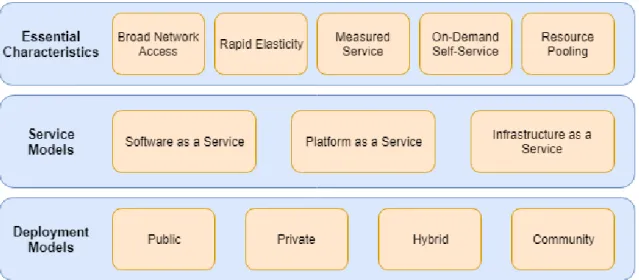
The NIST definition of cloud computing, in addition to the quotation at the beginning of the chapter, also lists five essential characteristics cloud computing services have, their three main service models, and four deployment models, shown in Figure 3.1, to support the definition. This chapter describes the NIST-listed essential characteristics of cloud computing in 3.1, then the deployment models in 3.2, and service models in 3.3.

(31)

Figure 3.1.NIST definition of cloud computing

3.1 Essential characteristics

The essential characteristicBroad Network Accessmeans, firstly that the resources pro-vided by the cloud are accessed through the internet. Secondly, it means that the me-chanics of accessing the resources are standard and promote use of any physical de-vices. [28] [9]

Rapid Elasticity means that the resources can be provisioned and upscaled or down-scaled quickly, and even automatically. The consumer does not see any physical resource limits of the provider, but rather is offered seemingly unlimited resources. [28] [9]

Measured Service means that the cloud-provided resources can be, and are measured and monitored actively. [28] The monitoring can be used by both the provider, for example to gather usage statistics, or by the consumer, for example to detect possible errors or to optimize provisioned resource amounts.

On-Demand Self-Service means that the consumer of a cloud service can provision re-sources independently, without needing any human interaction with the cloud service provider. [9][28]

Resource Pooling means pooling resources together, using a multi-tenant model or vir-tualization, to serve multiple consumers using any number and types of actual physical machines. [9] This essentially makes physical resources completely invisible to the con-sumers, making them not exactly or at all know where their computation or data storage is. [9] It also allows the provider to optimize the physical resources to match customer demands.

(32)

3.2 Deployment models

Private cloud is a cloud deployment model where the cloud infrastructure is used by a single organization. A private cloud might be hosted by the organization itself on-premise, or by a third-part provider. [28][9] Private cloud might be used because of security concerns or because the organization wants to be in full control of the cloud backend [9][21].

Community cloud is like private cloud in that it is used by an exclusive group of users, but unlike private cloud in that the users are from several different organizations. A com-munity cloud provides services which fulfill similar consumer needs between the organi-zations. It may be hosted by any of the user organizations or by a third party provider. [28][9]

Public cloud provices cloud services for open use by anyone [28], and is the most popular form of the deployment models [9]. A public cloud is managed and completely controlled by the cloud provider, which sets their own policies and charging models [9].

Ahybrid cloud solution tries to achieve the positives of both private and public clouds by combining two or more distinct cloud solutions. The combination is made by creating a solution between the individual clouds to make the data and applications in them portable between each other. [21][28]

In addition to the types listed by NIST, literature [49][9] often lists another solution, similar to hybrid cloud, which tries to combine public and private clouds’ good sides, calledVirtual private cloud. Virtual private cloud is a solution built on top of a public cloud which, using virtual private networks (VPN), makes it essentially private to consumers.

3.3 Service models

This section will explain the three main service models defined by NIST [28], shown in Figure 3.2, as well as a less-used termMachine learning as a service. The three service models are all different abstractions of resources that could be used as services of an own datacenter or software installed on own computer. Although Machine learning as a service is not a distinct abstraction level of resources provided, it is a distinct set of services that are often provided by cloud service providers, and that are much discussed and used in this thesis.

3.3.1 Infrastructure as a service

Infrastructure as a service (IaaS) is the lowest abstraction level of the service models. It aims to provide consumers the capabilities of a physical data center, without the customer

(33)

Figure 3.2. Cloud service model levels

needing to maintain a physical data center [21]. It provides the consumers with the fun-damental infrastructural resources like processing power, networks and storage, which the consumer can use as they see fit [28]. The consumer can use the provided resources to for example build a standard web application consisting of a database, server and a UI by using the provided storage to store the database and the server executable, using the provided processing power to run the server executable, and configuring the network so that users can access the UI from the Internet.

IaaS is typically implemented by heavily using virtualization to quickly provision or de-stroy resources according to consumer needs [9]. A common example [9, 21, 35] of an IaaS platform is Amazon Web Services EC2, a service which provides, as Amazon’s documentation [38] says, "virtual computing environments, known as instances". The instances can be configured from operating system upwards, and when created, can be used very similar to any normal remote computer by connecting to it using for example SSH [38].

(34)

3.3.2 Platform as a service

Platform as a service (PaaS) is an abstraction level on top of IaaS. A PaaS solution provides its users with an environment for developing and running applications. The environment contains support for a programming language and an assortment of libraries to use with it. In other words, PaaS offers consumers an application stack tailored for a purpose. [9][21][28]

A PaaS solution might for example provide a typical web server setup by offering a pre-defined database solution, an environment for running a server application in a specific programming language and framework, and serving the UI to users over the Internet in a configurable URL. An example of a PaaS which does just that is Heroku, which offers a variety of different programming languages and frameworks it knows how to run. One way of using Heroku is setting up a git repository which contains the web application code in a format Heroku knows, and git pushing the code to Heroku. [37]

3.3.3 Software as a service

Software as a service (SaaS) is the ultimate abstraction level of the service models. A SaaS solution provides the consumers with a complete, running application which can be accessed through the Internet. The only thing the consumer can configure are application-specific, with all the details of how the application is running hidden from them. [28]

SaaS solutions are plentiful on the Internet. Some of the common examples for them include enterprise resource planning (ERP) systems [21], and any web email client, for example Google Mail [9].

3.3.4 Machine learning as a service

Machine learning as a service (MLaaS) is not an abstraction level like the service models in the definition, but is a distinct set of services across previously mentioned service levels. Cloud providers [38][15][29] often provide a wide selection of SaaS-level services made possible by machine learning, like face detection from images, or turning speech audio into text. These services do not offer machine learning itself, but already trained models for common machine learning tasks.

The machine learning services themselves are usually PaaS-level solutions, which pro-vide interfaces with machine learning libraries. The model training process is abstracted, letting the users to focus on the data itself [34]. Cloud services often also provide ser-vices for storing the data itself, and transferring and transforming it between serser-vices. The machine learning services are also often supplemented by services for using the created

(35)

model for predictions after training. This can be done for example by creating a HTTP endpoint which returns the model prediction for a request containing input data.

(36)

4 IMPLEMENTATION

This chapter will discuss the implementation of the machine learning architecture out-lined in Chapter 1. First, the data and how it is used will be briefly discussed. Then, the requirements for the cloud service platform used are defined and listed. Then, the three biggest [35] cloud platforms are evaluated based on the requirements. Finally, one plat-form is chosen, and an architecture for implementing the machine learning applications will be presented.

4.1 Data

The data is stored in a relational database provided by Amazon Web Services. The data is operational in nature, and contains a history of work done in each worksite. The input data for the algorithm has to represent the state of the worksites in a static set of variables, which are not found in the database, and transformations have to be done first. To represent a state and history of a worksite in a set number of variables, a number of metrics are calculated from the operational data. Each worksite’s data is sampled with one hour intervals, removing hours of no work done to avoid duplicates. The metrics calculated from each of the hours will be an input data vector. So, if a worksite took ten working hours to complete, there will be ten rows in the final training data representing the different states of progression in that worksite.

A worksite’s completion time is modeled as hours of work needed before completion, which means a machine learning model’s output values is the number of working hours needed before the worksite is complete. This is much simpler to model than actual cal-endar completion time, and removes the need of handling actual dates and times. It also means that the algorithm will not be able to differentiate between worksites worked for example in different seasons. The hours of work needed before completion can only be calculated for already completed worksites, so the training data will only contain worksites completed before the extraction of the data. It is not a large setback however, as there are a lot more completed worksites than ones in progress.

(37)

4.2 Evaluation

The models are evaluated on two metrics: Mean squared error (MSE), and mean ab-solute error (MAE). All the models are trained minimizing mean squared error, as it is supported by all the model implementations used. Mean squared error tells straight how well the model minimized the loss value. Mean absolute error instead is a better esti-mate of how good the model is for its purpose, since mean squared error responds very strongly to outliers [44, p. 23], and eliminating a low amount of outliers is not as impor-tant as getting as good a prediction as possible for most of the worksites. Thus, mean absolute error is the metric used to choose the best model.

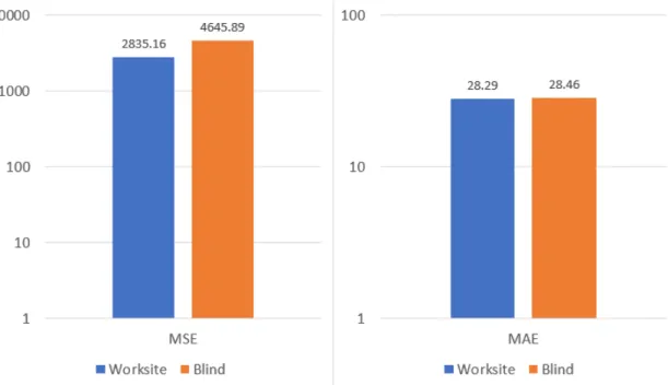
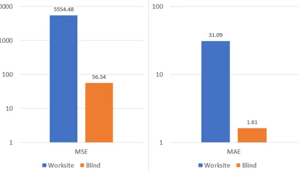
The data is split into 70% training data, and 30% test data. As there are multiple rows for each worksite in the whole data, there are two distinct ways of doing a random split. The first way, referred to as the worksitesplit, is made so that each worksite has all its data rows in either one set. The test set consists of roughly 30% of the worksites, and 30% of the total amount of the data rows. The second split, referred to as theblind split is made fully randomly, the test data consisting of 30% of the total amount of rows in the data. In the blind split, a worksite is likely to have its data both in the test set and the training set, which makes the task more of an interpolation than an extrapolation problem. The actual usage situation is an extrapolation problem, using past worksites’ data to predict an unseen worksite’s time of completion, so the worksite split is used for deciding the best machine learning model. The models are however tested with both splits, because the differences in their accuracy results can give insight into the quality of the parameter set extracted from the database.

4.3 Requirements

The first requirement for the cloud service platform is that it must be possible to implement all the machine learning models presented in Chapter 2 (Linear regression, Random forest, XGBoost and Multi-layer perceptron). All the models should be tested on a single platform to avoid having to create an architecture on multiple platforms.

The second requirement is that there must be a way to transform the data according to Section 4.1. The transformation cannot be done in the database, to keep the database only for operations. An integrated service built for transforming data is preferred to a general IaaS solution in which one would write a whole application for transforming the data.

The third requirement is that there must be a way to use the trained model for predictions after training. Although the architecture in this thesis is just a proof of concept, the same architecture should work if taken into production use. In its simplest, this could be just saving the model somewhere where another application can fetch the model and use it for predictions. However, an integrated solution is again preferred.

(38)

4.4 Platforms

This section will review the three biggest [35] cloud platforms from the viewpoint of fulfill-ing the requirements given in Section 4.3.

4.4.1 Amazon Web Services

Amazon Web Services (AWS) offers general machine learning services through a service called Amazon SageMaker. SageMaker enables building machine learning models, train-ing them, and hosttrain-ing them through HTTP endpoints. SageMaker offers multiple popular machine learning models built in. Of the models chosen for this thesis, XGBoost is of-fered built in. In addition, SageMaker offers library support for multiple machine learning frameworks. The additional frameworks include TensorFlow and PyTorch for creating and training neural networks, and Scikit-learn, which is capable of creating random forest and linear regression models [12]. Using the frameworks requires the user to write the training code themselves. For this purpose SageMaker offers Jupyter notebooks, where one may write the code in browser, and interactively run and test it. SageMaker is not designed to read data straight from a relational database, and needs something to create a file in AWS’s object storage service S3 (Simple Storage Service) first. [38]

For transforming data and moving it between services, AWS offers two services: Glue and Data Pipeline. Glue is an ETL (extract, transform, load) service, which is specifically made for moving data between different data stores. Glue works by reading data in data source chosen from different options, transforming it with a script written in either Spark (using Python or Scala as programming language) or pure Python, and saving it to a data target. The process can be automatically run on a schedule. Glue offers notebook instances in the same way as SageMaker for developing the scripts, and has crawler functionality for automatically determining the schema of the data source. Data Pipeline is a service for automating movement of data between services. Data Pipeline provides connections to multiple data sources like Glue, and offers simple scheduling tools for running the transfers. Data Pipeline is however not capable of doing complex transformations to the data by itself, but is instead more designed to be used together with dedicated analysis services, making the data available for them to use. [38]

4.4.2 Google Cloud

Google cloud offers general machine learning services as AI platform. AI platform is very similar to AWS SageMaker in that it offers Jupyter notebooks for writing scripts, and several frameworks as well as built-in algorithms for creating models. The built-in models include XGBoost, and the other required models are covered by the frameworks, including TensorFlow and Scikit-learn. AI Platform also offers hosting the trained models

(39)

for predictions. AI Platform does not provide a managed way to prepare data for training, and another service is needed for that. [15]

For data transformation and transfer, there is one main service provided in Google Cloud: Cloud Dataflow. Dataflow is a service for doing stream or batch transformations to data using Apache Beam, a data stream processing framework. Dataflow does not seem to have a managed interface for accessing a relational database though, and would require a dedicated program to fetch wanted data from the database and save it into the object storage service Cloud Storage first.

4.4.3 Microsoft Azure

Microsoft Azure has their general machine learning services in a service called Azure Machine Learning. Azure Machine Learning works similarly to the other cloud platforms’ corresponding services; it offers Jupyter notebooks for developing the machine learning scripts, with multiple machine learning frameworks. Azure Machine Learning software development kit supports Scikit-learn and TensorFlow, but XGBoost is not supported out-of-the-box. The service has possibility to use any framework of choice by using a general Estimator class, for which Python packages to install can be specified by name. [29] Data transformation from SQL database in Azure can be done via a service called Data Factory. Data Factory can create a connection between two data stores, and supported datastores include Azure’s object storage service, all Azure databases, multiple generic database and file system connections, and other cloud service providers’ services. Data Factory supports multiple data transformation frameworks, including Spark and MapRe-duce. [29]

4.5 Architecture

This section will describe the architecture of the machine learning application created for testing the different models. First, the choice of the implementation platform will be justi-fied, and then the data transformation achitecture and the machine learning architectures are separately presented.

4.5.1 Choice of platform

All of the cloud platforms listed in Section 4.4 are capable of the machine learning tasks required, although Azure requires a little more overhead, without the native support for XGBoost. The services in the platforms are in fact very similar to each other.

(40)

outline a clear way of extracting data from a SQL database. Azure and AWS both offer very similar ways of transforming data in SQL database into a CSV file accessible for the machine learning services. The machine learning architecture is implemented in AWS, as it offered the most managed and suitable services for the requirements. The operational data is also already stored in AWS, removing the step of copying it to somewhere else.

4.5.2 Data transformation

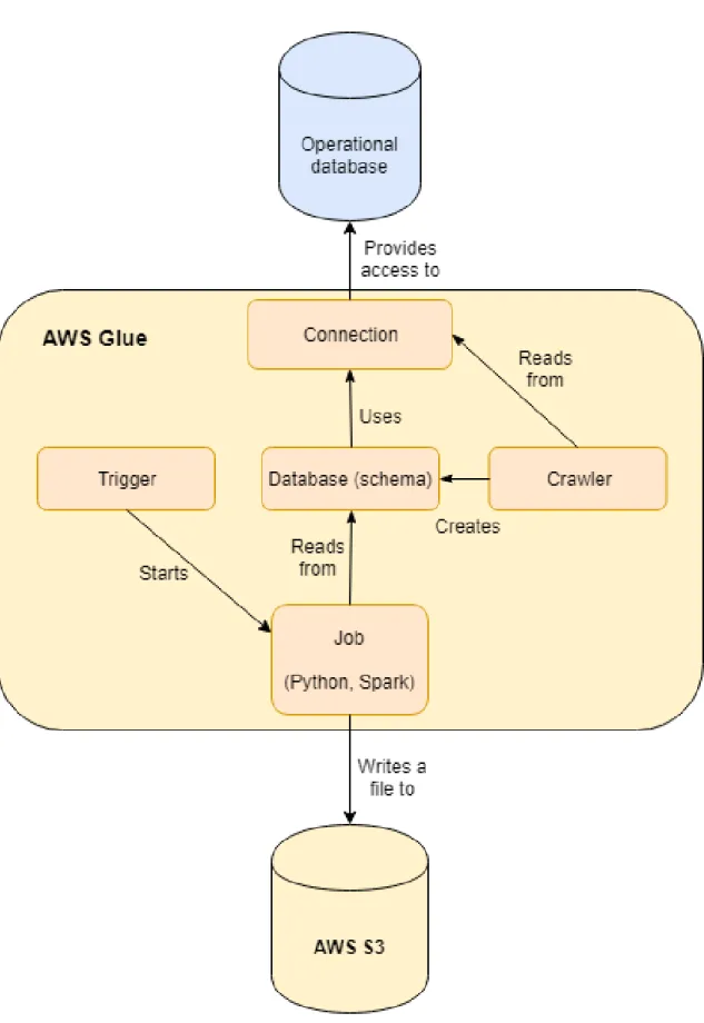
Data transformation is done using the AWS Glue service. AWS Glue consists of connec-tions, databases, crawlers, jobs, and triggers. A connection is simply the location of and credentials to the data store containing the input data. A database in Glue is a set of table definitions, which consist of the table schema containing column names and data types much like in SQL. All the table definitions are linked to a connection, to specify from where the data to the table should be fetched. Crawlers are a utility in Glue to automat-ically create table definitions for a database. A crawler is given a connection and some simple filters, and when run, it will create the table definitions for that connection.

Jobs are the main part of Glue. A job is a script written in either Spark or pure Python. Spark can be written using Python or Scala as the underlying language. A job reads data from Glue databases’ tables, does transformations on them, and writes the data some-where. In this thesis, the job reads data from the SQL database, does the hourly sampling described in Section 4.1, finds the features and the target values, and writes them as a single CSV file in AWS S3. A job can be automatically run with trigger functionality in Glue. A trigger can be configured to execute on a schedule, on a set of job events like failure or success, or on demand. In a production application, the job would be run on a scheduled trigger, but in this proof of concept architecture, they are not used, and the job is run by hand. The whole Glue process is illustrated in Figure 4.1.

4.5.3 Machine learning

Machine learning is implemented in AWS SageMaker. SageMaker is a managed machine learning service which provides tools to develop, train and deploy a machine learning model. For this thesis’s purposes, SageMaker consists of training jobs, models, end-points, and notebooks.

A training job contains all the needed instructions for creating and training a model. The information is the algorithm definition, input data configuration, output data configuration, and hyperparameters. An algorithm definition defines which machine learning model will be created when the job is run. A definition is linked to a training image in AWS Elastic Container Registry (ECR), which contains a docker image with all the needed programming languages and libraries for the algorithm. Algorithm definition also defined which AWS virtual machine (instance) type to use for training. There are multiple to

(41)